Flash-Flood Potential Mapping Using Deep Learning, Alternating Decision Trees and Data Provided by Remote Sensing Sensors

 ,
,  ,
,  , ,
, ,  ,
,  , ,
, ,
Abstract
:1. Introduction
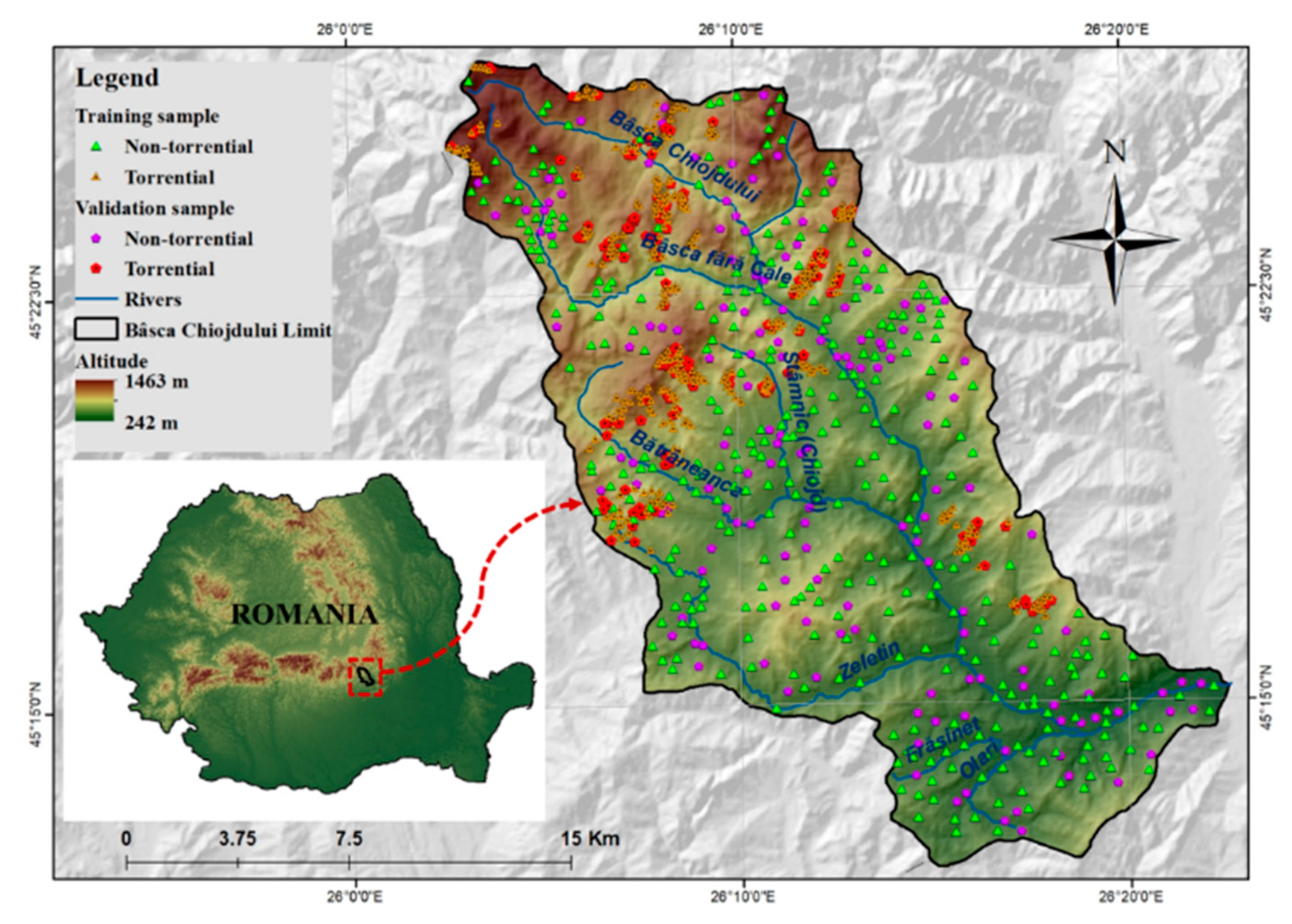
2. Study Area
3. Data
3.1. Torrential Area Inventory and Sampling
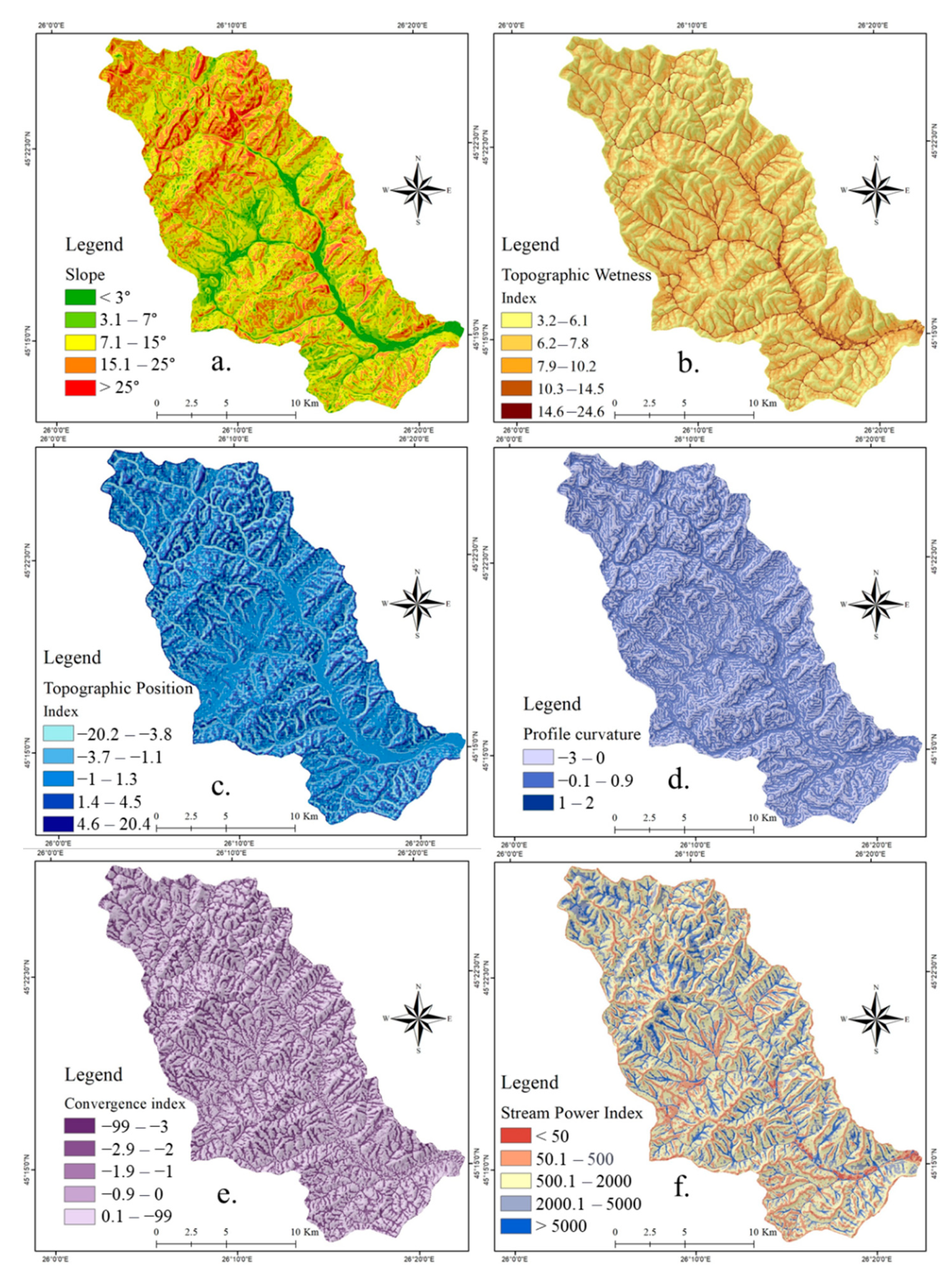
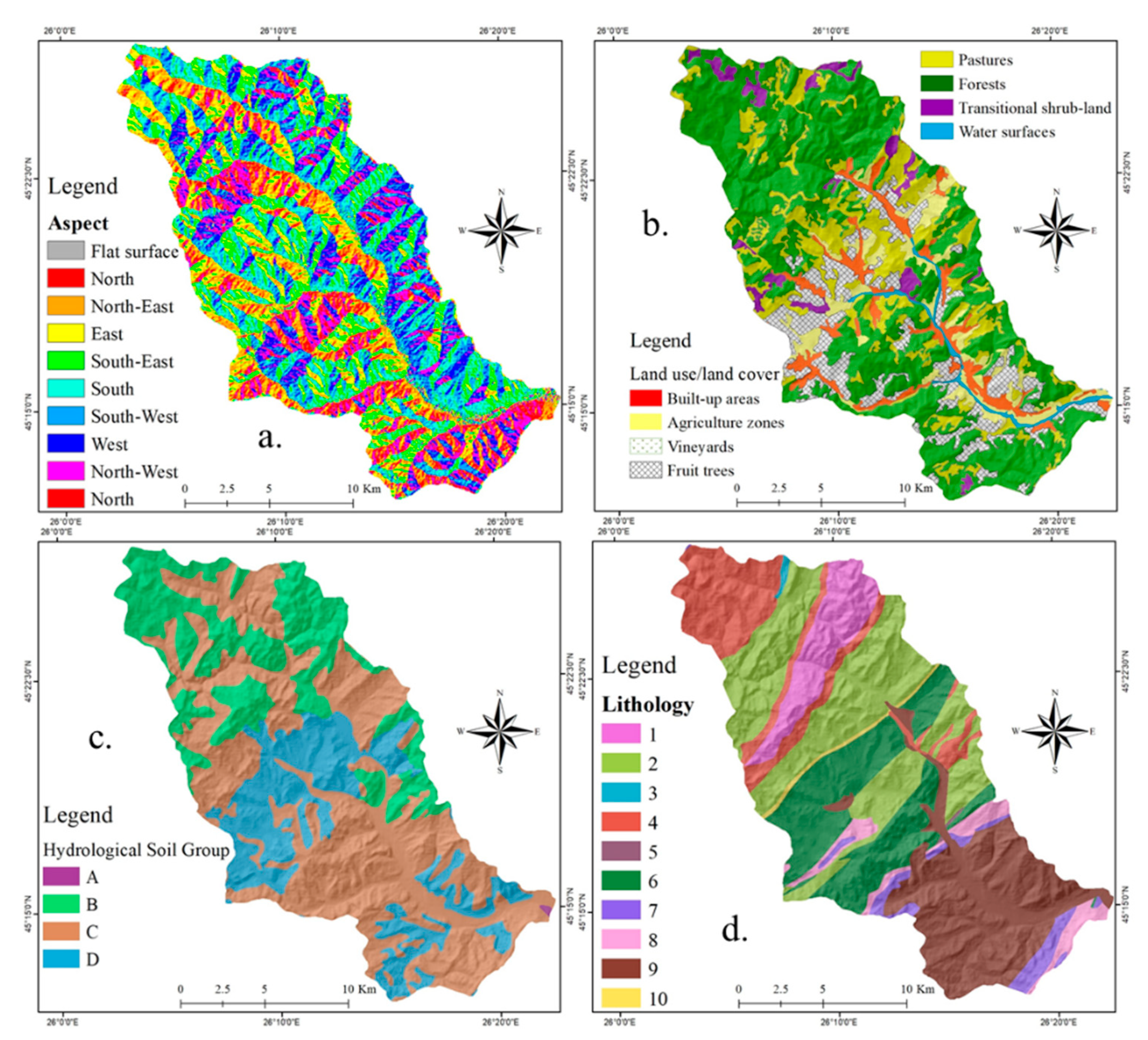
3.2. Flash-Flood Predictors
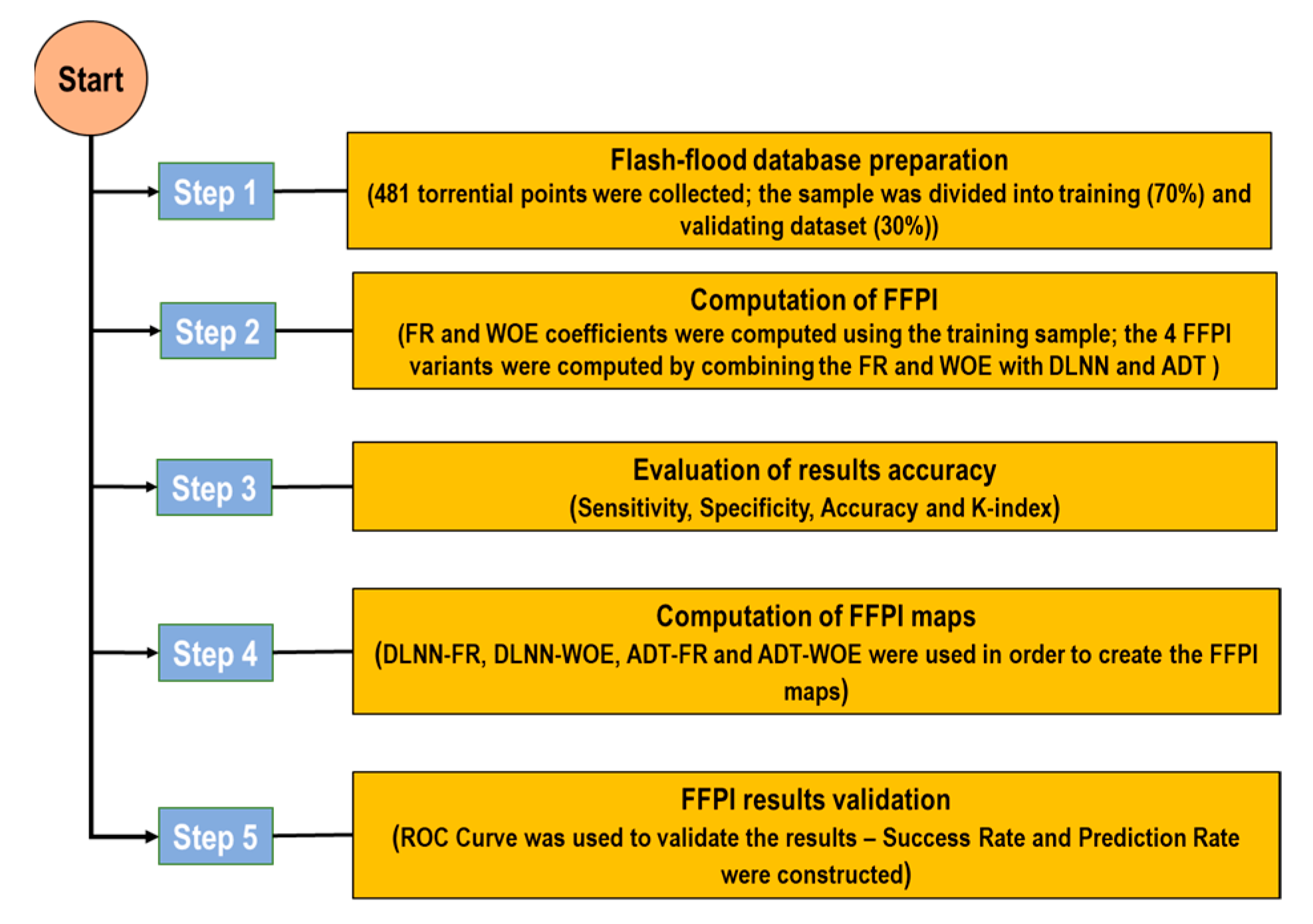
4. Methods
4.1. Linear Support Vector Machine (LSVM) for Feature Selection
4.2. Weights of Evidence (WOE)
4.3. Frequency Ratio (FR)
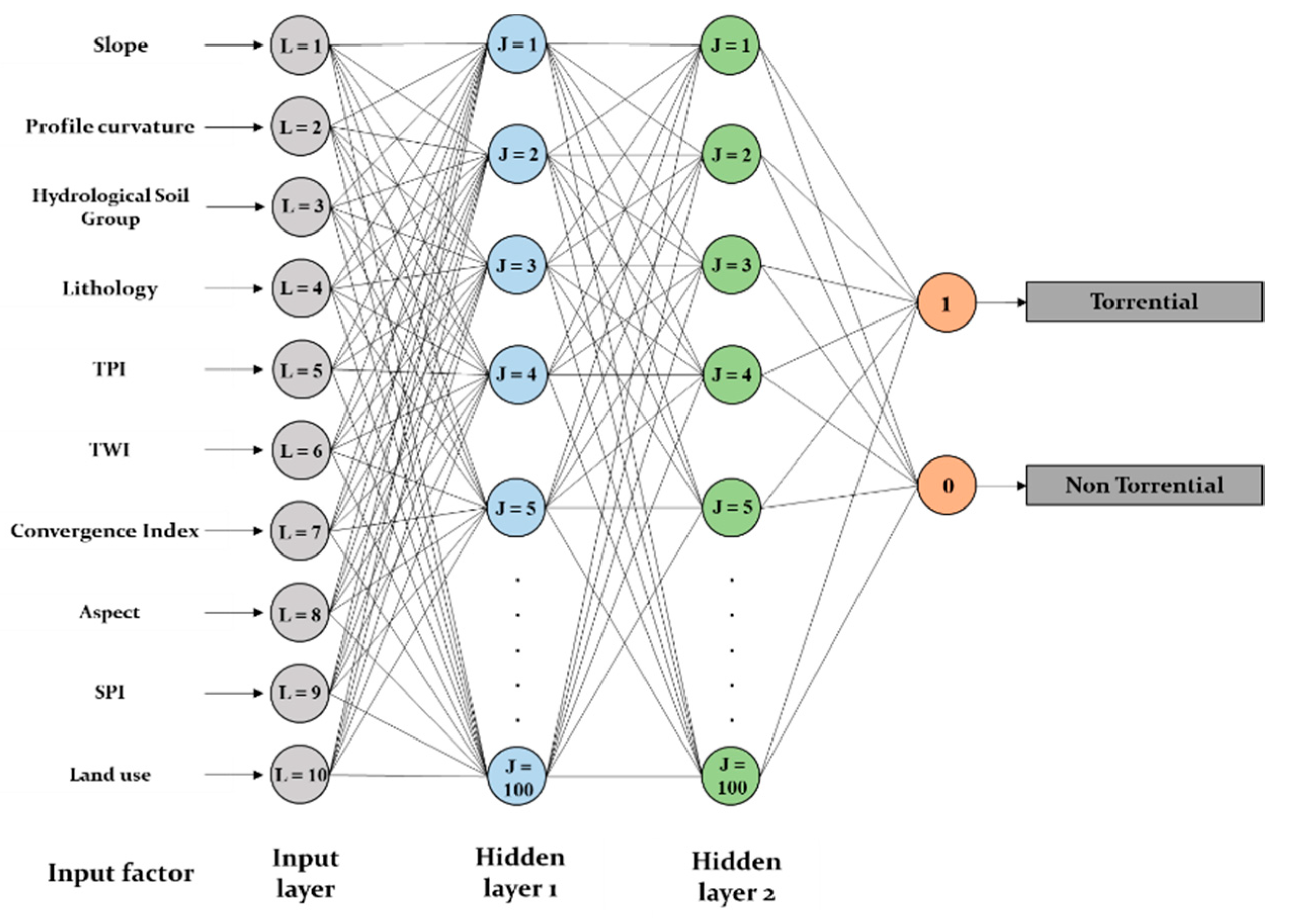
4.4. Deep Learning Neural Network (DLNN)
4.5. Alternating Decision Tree
4.6. Model Performance and Results Validation
4.6.1. Statistical Measures
4.6.2. ROC Curve
5. Results
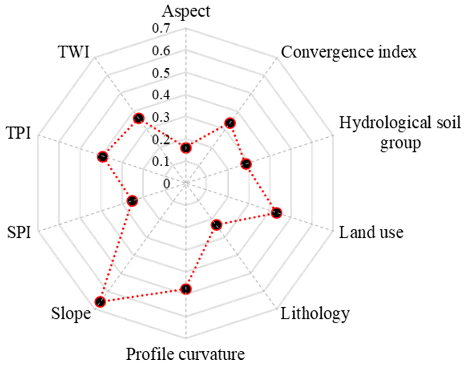
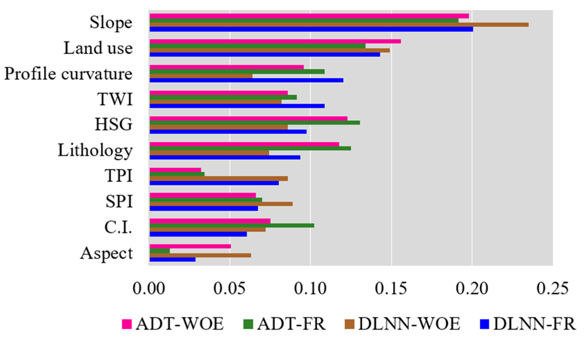
5.1. Feature Selection Using LSVM
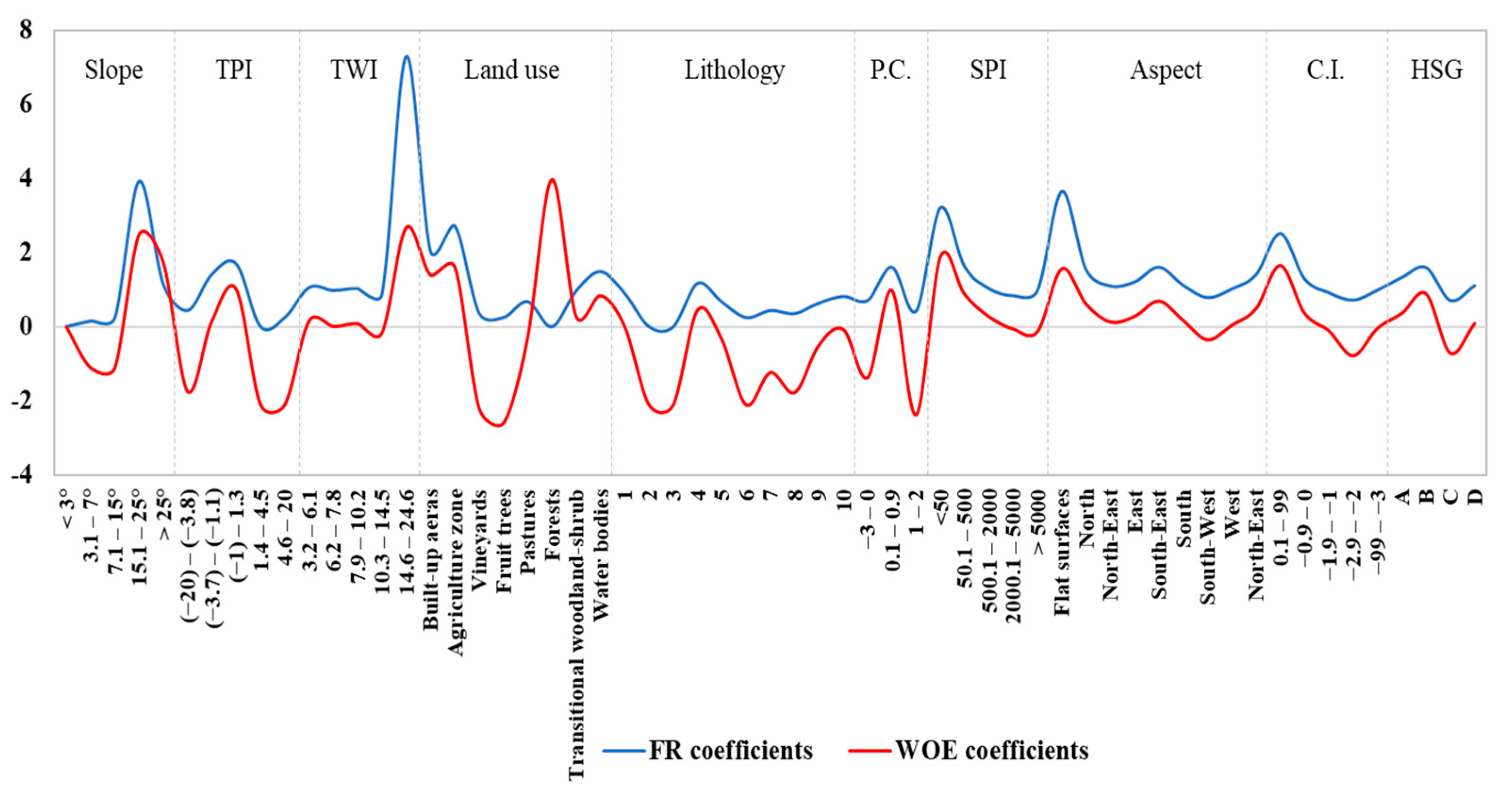
5.2. FR and WOE Coefficients
5.3. Models Performance Assessment
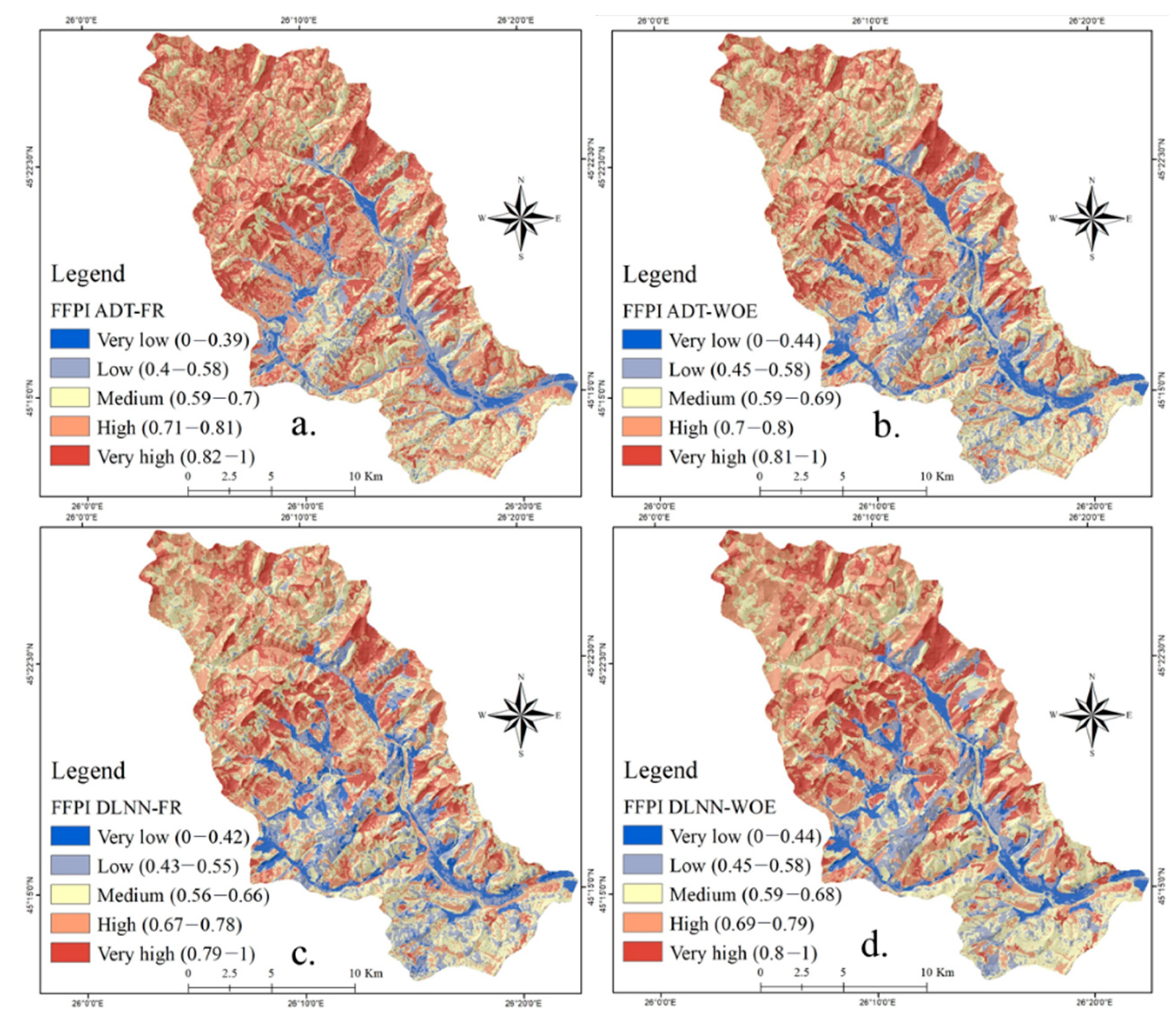
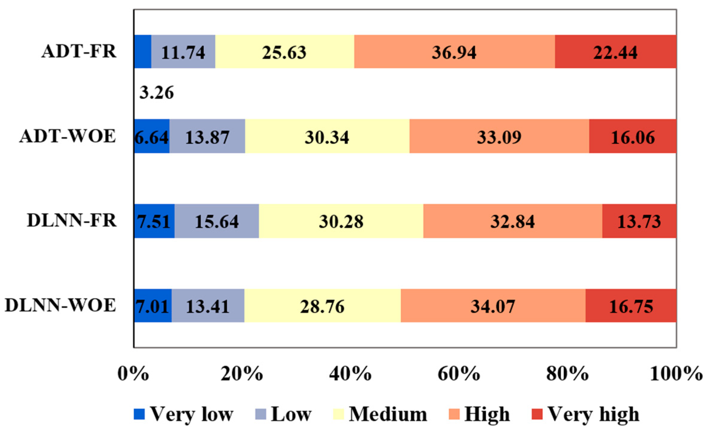
5.4. Results of Machine Learning Ensembles
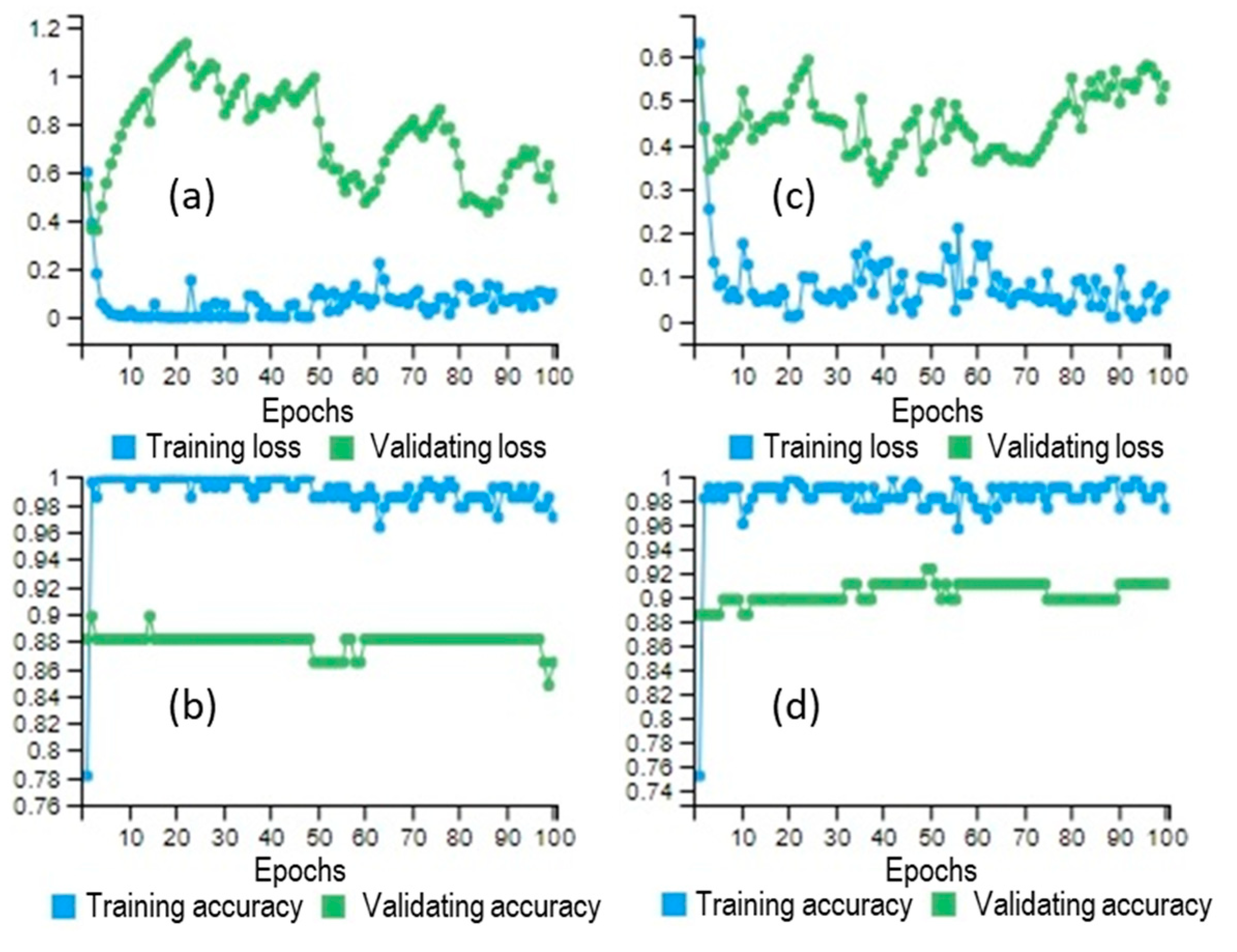
5.4.1. DLNN-FR and DLNN-WOE Results
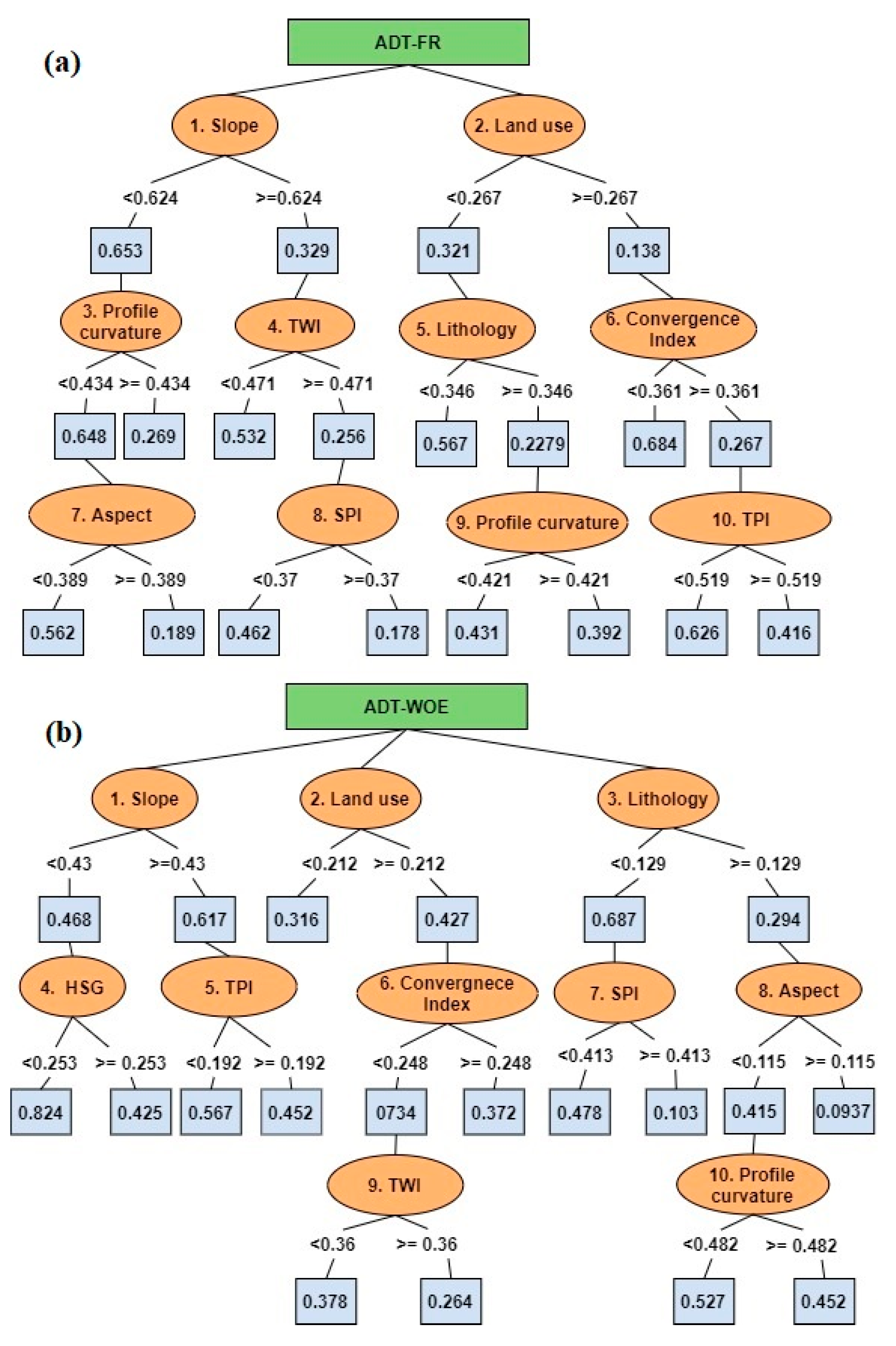
5.4.2. ADT-FR and ADT-WOE Results
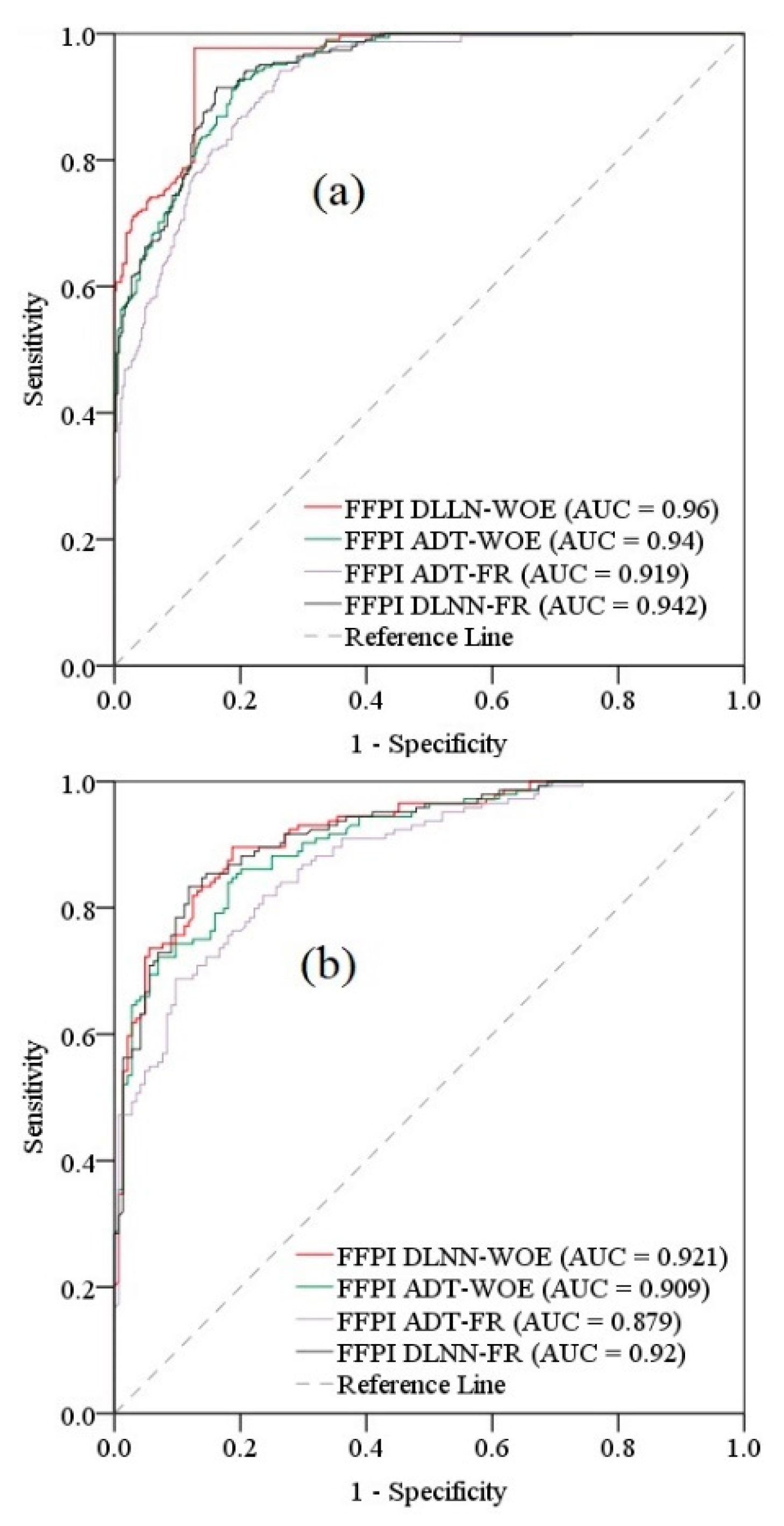
5.5. Results Validation Using ROC Curve
6. Discussions
7. Conclusions
Author Contributions
Funding
Institutional Review Board Statement
Informed Consent Statement
Data Availability Statement
Conflicts of Interest
References
- Halkos, G.; Skouloudis, A. Investigating resilience barriers of small and medium-sized enterprises to flash floods: A quantile regression of determining factors. Clim. Dev. 2020, 12, 57–66. [Google Scholar] [CrossRef]
- Bezak, N.; Mikoš, M. Investigation of Trends, Temporal Changes in Intensity-Duration-Frequency (IDF) Curves and Extreme Rainfall Events Clustering at Regional Scale Using 5 min Rainfall Data. Water 2019, 11, 2167. [Google Scholar] [CrossRef] [Green Version]
- Bui, D.T.; Tsangaratos, P.; Ngo, P.-T.T.; Pham, T.D.; Pham, B.T. Flash flood susceptibility modeling using an optimized fuzzy rule based feature selection technique and tree based ensemble methods. Sci. Total Environ. 2019, 668, 1038–1054. [Google Scholar] [CrossRef] [PubMed]
- Cao, C.; Xu, P.; Wang, Y.; Chen, J.; Zheng, L.; Niu, C. Flash flood hazard susceptibility mapping using frequency ratio and statistical index methods in coalmine subsidence areas. Sustainability 2016, 8, 948. [Google Scholar] [CrossRef] [Green Version]
- Costache, R. Flash-Flood Potential assessment in the upper and middle sector of Prahova river catchment (Romania). A comparative approach between four hybrid models. Sci. Total Environ. 2019, 659, 1115–1134. [Google Scholar] [CrossRef]
- Elkhrachy, I. Flash flood hazard mapping using satellite images and GIS tools: A case study of Najran City, Kingdom of Saudi Arabia (KSA). Egypt. J. Remote Sens. Space Sci. 2015, 18, 261–278. [Google Scholar] [CrossRef] [Green Version]
- Costache, R.; Bui, D.T. Identification of areas prone to flash-flood phenomena using multiple-criteria decision-making, bivariate statistics, machine learning and their ensembles. Sci. Total Environ. 2020, 712, 136492. [Google Scholar] [CrossRef]
- Janizadeh, S.; Avand, M.; Jaafari, A.; Phong, T.V.; Bayat, M.; Ahmadisharaf, E.; Prakash, I.; Pham, B.T.; Lee, S. Prediction Success of Machine Learning Methods for Flash Flood Susceptibility Mapping in the Tafresh Watershed, Iran. Sustainability 2019, 11, 5426. [Google Scholar] [CrossRef] [Green Version]
- Hosseini, F.S.; Choubin, B.; Mosavi, A.; Nabipour, N.; Shamshirband, S.; Darabi, H.; Haghighi, A.T. Flash-flood hazard assessment using ensembles and Bayesian-based machine learning models: Application of the simulated annealing feature selection method. Sci. Total Environ. 2020, 711, 135161. [Google Scholar] [CrossRef]
- Liu, Y.-X.; Yang, C.-N.; Sun, Q.-D.; Wu, S.-Y.; Lin, S.-S.; Chou, Y.-S. Enhanced embedding capacity for the SMSD-based data-hiding method. Signal Process. Image Commun. 2019, 78, 216–222. [Google Scholar] [CrossRef]
- Zhao, C.; Li, J. Equilibrium Selection under the Bayes-Based Strategy Updating Rules. Symmetry 2020, 12, 739. [Google Scholar] [CrossRef]
- Xiong, Q.; Zhang, X.; Wang, W.-F.; Gu, Y. A Parallel Algorithm Framework for Feature Extraction of EEG Signals on MPI. Comput. Math. Methods Med. 2020, 2020, 9812019. [Google Scholar] [CrossRef] [PubMed]
- Zhu, Q. Research on Road Traffic Situation Awareness System Based on Image Big Data. IEEE Intell. Syst. 2019, 35, 18–26. [Google Scholar] [CrossRef]
- Fu, X.; Yang, Y. Modeling and analysis of cascading node-link failures in multi-sink wireless sensor networks. Reliab. Eng. Syst. Saf. 2020, 197, 106815. [Google Scholar] [CrossRef]
- Fu, X.; Pace, P.; Aloi, G.; Yang, L.; Fortino, G. Topology Optimization Against Cascading Failures on Wireless Sensor Networks Using a Memetic Algorithm. Comput. Netw. 2020, 177, 107327. [Google Scholar] [CrossRef]
- Zenggang, X.; Zhiwen, T.; Xiaowen, C.; Xue-min, Z.; Kaibin, Z.; Conghuan, Y. Research on Image Retrieval Algorithm Based on Combination of Color and Shape Features. J. Signal Process. Syst. 2019, 1–8. [Google Scholar] [CrossRef]
- Zuo, C.; Sun, J.; Li, J.; Asundi, A.; Chen, Q. Wide-field high-resolution 3d microscopy with fourier ptychographic diffraction tomography. Opt. Lasers Eng. 2020, 128, 106003. [Google Scholar] [CrossRef] [Green Version]
- Long, Q.; Wu, C.; Wang, X. A system of nonsmooth equations solver based upon subgradient method. Appl. Math. Comput. 2015, 251, 284–299. [Google Scholar] [CrossRef]
- Zhu, J.; Shi, Q.; Wu, P.; Sheng, Z.; Wang, X. Complexity analysis of prefabrication contractors’ dynamic price competition in mega projects with different competition strategies. Complexity 2018, 2018, 5928235. [Google Scholar] [CrossRef]
- Xiong, L.; Zhang, H.; Li, Y.; Liu, Z. Improved stability and H∞ performance for neutral systems with uncertain Markovian jump. Nonlinear Anal. Hybrid Systems 2016, 19, 13–25. [Google Scholar]
- Wu, T.; Cao, J.; Xiong, L.; Zhang, H. New Stabilization Results for Semi-Markov Chaotic Systems with Fuzzy Sampled-Data Control. Complexity 2019, 2019, 7875305. [Google Scholar] [CrossRef]
- Wu, T.; Xiong, L.; Cheng, J.; Xie, X. New results on stabilization analysis for fuzzy semi-Markov jump chaotic systems with state quantized sampled-data controller. Inf. Sci. 2020, 521, 231–250. [Google Scholar] [CrossRef]
- Shi, K.; Wang, J.; Tang, Y.; Zhong, S. Reliable asynchronous sampled-data filtering of T–S fuzzy uncertain delayed neural networks with stochastic switched topologies. Fuzzy Sets Syst. 2020, 381, 1–25. [Google Scholar] [CrossRef]
- Shi, K.; Wang, J.; Zhong, S.; Tang, Y.; Cheng, J. Non-fragile memory filtering of TS fuzzy delayed neural networks based on switched fuzzy sampled-data control. Fuzzy Sets Syst. 2020, 394, 40–64. [Google Scholar] [CrossRef]
- Xu, M.; Li, T.; Wang, Z.; Deng, X.; Yang, R.; Guan, Z. Reducing complexity of HEVC: A deep learning approach. IEEE Trans. Image Process. 2018, 27, 5044–5059. [Google Scholar] [CrossRef] [Green Version]
- Lv, Z.; Qiao, L. Deep belief network and linear perceptron based cognitive computing for collaborative robots. Appl. Soft Comput. 2020, 92, 106300. [Google Scholar] [CrossRef]
- Lv, Z.; Xiu, W. Interaction of edge-cloud computing based on SDN and NFV for next generation IoT. IEEE Internet Things J. 2019, 7, 5706–5712. [Google Scholar] [CrossRef]
- Chen, H.; Chen, A.; Xu, L.; Xie, H.; Qiao, H.; Lin, Q.; Cai, K. A deep learning CNN architecture applied in smart near-infrared analysis of water pollution for agricultural irrigation resources. Agric. Water Manag. 2020, 240, 106303. [Google Scholar] [CrossRef]
- Chen, H.; Qiao, H.; Xu, L.; Feng, Q.; Cai, K. A Fuzzy Optimization Strategy for the Implementation of RBF LSSVR Model in Vis–NIR Analysis of Pomelo Maturity. IEEE Trans. Ind. Inform. 2019, 15, 5971–5979. [Google Scholar] [CrossRef]
- Qian, J.; Feng, S.; Tao, T.; Hu, Y.; Li, Y.; Chen, Q.; Zuo, C. Deep-learning-enabled geometric constraints and phase unwrapping for single-shot absolute 3D shape measurement. APL Photonics 2020, 5, 046105. [Google Scholar] [CrossRef]
- Qian, J.; Feng, S.; Li, Y.; Tao, T.; Han, J.; Chen, Q.; Zuo, C. Single-shot absolute 3D shape measurement with deep-learning-based color fringe projection profilometry. Opt. Lett. 2020, 45, 1842–1845. [Google Scholar] [CrossRef] [PubMed]
- Chao, L.; Zhang, K.; Li, Z.; Zhu, Y.; Wang, J.; Yu, Z. Geographically weighted regression based methods for merging satellite and gauge precipitation. J. Hydrol. 2018, 558, 275–289. [Google Scholar] [CrossRef]
- Zhang, S.; Pak, R.Y.; Zhang, J. Vertical time-harmonic coupling vibration of an impermeable, rigid, circular plate resting on a finite, poroelastic soil layer. Acta Geotech. 2020, 1–25. [Google Scholar]
- Yang, S.; Deng, B.; Wang, J.; Li, H.; Lu, M.; Che, Y.; Wei, X.; Loparo, K.A. Scalable Digital Neuromorphic Architecture for Large-Scale Biophysically Meaningful Neural Network with Multi-Compartment Neurons. IEEE Trans. Neural Netw. Learn. Syst. 2019, 1–15. [Google Scholar] [CrossRef] [PubMed]
- Tsai, Y.H.; Wang, J.; Chien, W.T.; Wei, C.Y.; Wang, X.; Hsieh, S.H. A BIM-based approach for predicting corrosion under insulation. Autom. Constr. 2019, 107, 102923. [Google Scholar] [CrossRef]
- Costache, R.; Zaharia, L. Flash-flood potential assessment and mapping by integrating the weights-of-evidence and frequency ratio statistical methods in GIS environment–case study: Bâsca Chiojdului River catchment (Romania). J. Earth Syst. Sci. 2017, 126, 59. [Google Scholar] [CrossRef]
- Khosravi, K.; Nohani, E.; Maroufinia, E.; Pourghasemi, H.R. A GIS-based flood susceptibility assessment and its mapping in Iran: A comparison between frequency ratio and weights-of-evidence bivariate statistical models with multi-criteria decision-making technique. Nat. Hazards 2016, 83, 947–987. [Google Scholar] [CrossRef]
- Costache, R.; Hong, H.; Pham, Q.B. Comparative assessment of the flash-flood potential within small mountain catchments using bivariate statistics and their novel hybrid integration with machine learning models. Sci. Total Environ. 2020, 711, 134514. [Google Scholar] [CrossRef]
- Tien Bui, D.; Khosravi, K.; Shahabi, H.; Daggupati, P.; Adamowski, J.F.; Melesse, A.M.; Thai Pham, B.; Pourghasemi, H.R.; Mahmoudi, M.; Bahrami, S. Flood spatial modeling in northern Iran using remote sensing and gis: A comparison between evidential belief functions and its ensemble with a multivariate logistic regression model. Remote Sens. 2019, 11, 1589. [Google Scholar] [CrossRef] [Green Version]
- Razandi, Y.; Pourghasemi, H.R.; Neisani, N.S.; Rahmati, O. Application of analytical hierarchy process, frequency ratio, and certainty factor models for groundwater potential mapping using GIS. Earth Sci. Inform. 2015, 8, 867–883. [Google Scholar] [CrossRef]
- Siahkamari, S.; Haghizadeh, A.; Zeinivand, H.; Tahmasebipour, N.; Rahmati, O. Spatial prediction of flood-susceptible areas using frequency ratio and maximum entropy models. Geocarto Int. 2018, 33, 927–941. [Google Scholar] [CrossRef]
- Yang, W.; Xu, K.; Lian, J.; Ma, C.; Bin, L. Integrated flood vulnerability assessment approach based on TOPSIS and Shannon entropy methods. Ecol. Indic. 2018, 89, 269–280. [Google Scholar] [CrossRef]
- Razavi Termeh, S.V.; Pourghasemi, H.R.; Alidadganfard, F. Flood Inundation Susceptibility Mapping using Analytical Hierarchy Process (AHP) and TOPSIS Decision Making Methods and Weight of Evidence Statistical Model (Case Study: Jahrom Township, Fars Province). J. Watershed Manag. Res. 2018, 9, 67–81. [Google Scholar] [CrossRef]
- Dano, U.L.; Balogun, A.-L.; Matori, A.-N.; Wan Yusouf, K.; Abubakar, I.R.; Said Mohamed, M.A.; Aina, Y.A.; Pradhan, B. Flood susceptibility mapping using GIS-based analytic network process: A case study of Perlis, Malaysia. Water 2019, 11, 615. [Google Scholar] [CrossRef] [Green Version]
- Khosravi, K.; Shahabi, H.; Pham, B.T.; Adamowski, J.; Shirzadi, A.; Pradhan, B.; Dou, J.; Ly, H.-B.; Gróf, G.; Ho, H.L. A comparative assessment of flood susceptibility modeling using Multi-Criteria Decision-Making Analysis and Machine Learning Methods. J. Hydrol. 2019, 573, 311–323. [Google Scholar] [CrossRef]
- Ali, S.A.; Parvin, F.; Pham, Q.B.; Vojtek, M.; Vojteková, J.; Costache, R.; Linh, N.T.T.; Nguyen, H.Q.; Ahmad, A.; Ghorbani, M.A. GIS-based comparative assessment of flood susceptibility mapping using hybrid multi-criteria decision-making approach, naïve Bayes tree, bivariate statistics and logistic regression: A case of Topľa basin, Slovakia. Ecol. Indic. 2020, 117, 106620. [Google Scholar] [CrossRef]
- Chen, W.; Li, Y.; Xue, W.; Shahabi, H.; Li, S.; Hong, H.; Wang, X.; Bian, H.; Zhang, S.; Pradhan, B. Modeling flood susceptibility using data-driven approaches of naïve bayes tree, alternating decision tree, and random forest methods. Sci. Total Environ. 2020, 701, 134979. [Google Scholar] [CrossRef]
- Chapi, K.; Singh, V.P.; Shirzadi, A.; Shahabi, H.; Bui, D.T.; Pham, B.T.; Khosravi, K. A novel hybrid artificial intelligence approach for flood susceptibility assessment. Environ. Model. Softw. 2017, 95, 229–245. [Google Scholar] [CrossRef]
- Avand, M.; Janizadeh, S.; Naghibi, S.A.; Pourghasemi, H.R.; Khosrobeigi Bozchaloei, S.; Blaschke, T. A Comparative Assessment of Random Forest and k-Nearest Neighbor Classifiers for Gully Erosion Susceptibility Mapping. Water 2019, 11, 2076. [Google Scholar] [CrossRef] [Green Version]
- Pham, B.T.; Prakash, I.; Bui, D.T. Spatial prediction of landslides using a hybrid machine learning approach based on random subspace and classification and regression trees. Geomorphology 2018, 303, 256–270. [Google Scholar] [CrossRef]
- Choubin, B.; Moradi, E.; Golshan, M.; Adamowski, J.; Sajedi-Hosseini, F.; Mosavi, A. An Ensemble prediction of flood susceptibility using multivariate discriminant analysis, classification and regression trees, and support vector machines. Sci. Total Environ. 2019, 651, 2087–2096. [Google Scholar] [CrossRef] [PubMed]
- Wang, Y.; Hong, H.; Chen, W.; Li, S.; Panahi, M.; Khosravi, K.; Shirzadi, A.; Shahabi, H.; Panahi, S.; Costache, R. Flood susceptibility mapping in Dingnan County (China) using adaptive neuro-fuzzy inference system with biogeography based optimization and imperialistic competitive algorithm. J. Environ. Manag. 2019, 247, 712–729. [Google Scholar] [CrossRef] [PubMed]
- Costache, R.; Pham, Q.B.; Sharifi, E.; Linh, N.T.T.; Abba, S.; Vojtek, M.; Vojteková, J.; Nhi, P.T.T.; Khoi, D.N. Flash-Flood Susceptibility Assessment Using Multi-Criteria Decision Making and Machine Learning Supported by Remote Sensing and GIS Techniques. Remote Sens. 2020, 12, 106. [Google Scholar] [CrossRef] [Green Version]
- Bui, D.T.; Hoang, N.-D.; Martínez-Álvarez, F.; Ngo, P.-T.T.; Hoa, P.V.; Pham, T.D.; Samui, P.; Costache, R. A novel deep learning neural network approach for predicting flash flood susceptibility: A case study at a high frequency tropical storm area. Sci. Total Environ. 2020, 701, 134413. [Google Scholar]
- Arabameri, A.; Saha, S.; Chen, W.; Roy, J.; Pradhan, B.; Bui, D.T. Flash flood susceptibility modelling using functional tree and hybrid ensemble techniques. J. Hydrol. 2020, 587, 125007. [Google Scholar] [CrossRef]
- Tehrany, M.S.; Pradhan, B.; Jebur, M.N. Flood susceptibility mapping using a novel ensemble weights-of-evidence and support vector machine models in GIS. J. Hydrol. 2014, 512, 332–343. [Google Scholar] [CrossRef]
- Prăvălie, R.; Costache, R. The analysis of the susceptibility of the flash-floods’ genesis in the area of the hydrographical basin of Bāsca Chiojdului river/Analiza susceptibilitatii genezei viiturilor īn aria bazinului hidrografic al rāului Bāsca Chiojdului. Forum Geogr. 2014, 13, 39–49. [Google Scholar] [CrossRef]
- Zarea, R.; Gheorghe, M. Dangerous hydrological phenomena on the Hydrographic Basin Bâsca Chiojdului. In Buletinul Institutului Politehnic Din Iaşi; Universitatea Tehnică “Gheorghe Asachi” din Iaşi Tomul LVI (LX), Fasc: Iași, Romania, 2010; pp. 37–48. [Google Scholar]
- Prăvălie, R.; Costache, R. Assessment of socioeconomic vulnerability to floods in the Bâsca Chiojdului catchment area. Rom. Rev. Reg. Stud. 2014, 10, 2. [Google Scholar]
- Chen, W.; Li, W.; Chai, H.; Hou, E.; Li, X.; Ding, X. GIS-based landslide susceptibility mapping using analytical hierarchy process (AHP) and certainty factor (CF) models for the Baozhong region of Baoji City, China. Environ. Earth Sci. 2016, 75, 63. [Google Scholar] [CrossRef]
- Costache, R. Flash-flood Potential Index mapping using weights of evidence, decision Trees models and their novel hybrid integration. Stoch. Environ. Res. Risk Assess. 2019, 33, 1375–1402. [Google Scholar] [CrossRef]
- Skentos, A. Topographic Position Index based landform analysis of Messaria (Ikaria Island, Greece). Acta Geobalcanica 2018, 4, 7–15. [Google Scholar] [CrossRef]
- Bui, D.T.; Pradhan, B.; Revhaug, I.; Tran, C.T. A comparative assessment between the application of fuzzy unordered rules induction algorithm and J48 decision tree models in spatial prediction of shallow landslides at Lang Son City, Vietnam. In Remote Sensing Applications in Environmental Research; Springer: Berlin/Heidelberg, Germany, 2014; pp. 87–111. [Google Scholar]
- De Rosa, P.; Fredduzzi, A.; Cencetti, C. Stream Power Determination in GIS: An Index to Evaluate the Most’Sensitive’Points of a River. Water 2019, 11, 1145. [Google Scholar] [CrossRef] [Green Version]
- Corrao, M.V.; Link, T.E.; Heinse, R.; Eitel, J.U. Modeling of terracette-hillslope soil moisture as a function of aspect, slope and vegetation in a semi-arid environment. Earth Surf. Process. Landf. 2017, 42, 1560–1572. [Google Scholar] [CrossRef]
- Zhang, K.; Ruben, G.B.; Li, X.; Li, Z.; Yu, Z.; Xia, J.; Dong, Z. A comprehensive assessment framework for quantifying climatic and anthropogenic contributions to streamflow changes: A case study in a typical semi-arid North China basin. Environ. Model. Softw. 2020, 104704. [Google Scholar] [CrossRef]
- Zhang, K.; Wang, Q.; Chao, L.; Ye, J.; Li, Z.; Yu, Z.; Yang, T.; Ju, Q. Ground Observation-based Analysis of Soil Moisture Spatiotemporal Variability Across A Humid to Semi-Humid Transitional Zone in China. J. Hydrol. 2019, 574, 903–914. [Google Scholar] [CrossRef]
- Singh, C.; Walia, E.; Kaur, K.P. Enhancing color image retrieval performance with feature fusion and non-linear support vector machine classifier. Optik 2018, 158, 127–141. [Google Scholar] [CrossRef]
- Lin, S.-W.; Lee, Z.-J.; Chen, S.-C.; Tseng, T.-Y. Parameter determination of support vector machine and feature selection using simulated annealing approach. Appl. Soft Comput. 2008, 8, 1505–1512. [Google Scholar] [CrossRef]
- Lee, S.; Kim, Y.-S.; Oh, H.-J. Application of a weights-of-evidence method and GIS to regional groundwater productivity potential mapping. J. Environ. Manag. 2012, 96, 91–105. [Google Scholar] [CrossRef]
- Van Westen, C. Statistical Landslide Hazards Analysis, ILWIS 2.1 for Windows Application Guide; International Institute for Aerospace Survey and Earth Sciences (ITC) Publication: Enschede, The Netherlands, 1997. [Google Scholar]
- Lee, S.; Pradhan, B. Landslide hazard mapping at Selangor, Malaysia using frequency ratio and logistic regression models. Landslides 2007, 4, 33–41. [Google Scholar] [CrossRef]
- Nielsen, M.A. Neural Networks and Deep Learning; Determination Press: San Francisco, CA, USA, 2015; Volume 25. [Google Scholar]
- Schmidhuber, J. Deep learning in neural networks: An overview. Neural Netw. 2015, 61, 85–117. [Google Scholar] [CrossRef] [Green Version]
- Agarap, A.F. Deep learning using rectified linear units (relu). arXiv 2018, arXiv:180308375. [Google Scholar]
- Bui, Q.-T.; Nguyen, Q.-H.; Nguyen, X.L.; Pham, V.D.; Nguyen, H.D.; Pham, V.-M. Verification of novel integrations of swarm intelligence algorithms into deep learning neural network for flood susceptibility mapping. J. Hydrol. 2020, 581, 124379. [Google Scholar] [CrossRef]
- Huang, Z.; Li, J.; Weng, C.; Lee, C.-H. Beyond Cross-Entropy: Towards Better Frame-Level Objective Functions for Deep Neural Network Training in Automatic Speech Recognition. In Proceedings of the INTERSPEECH—15th Annual Conference of the International Speech Communication Association, Singapore, 14–18 September 2014. [Google Scholar]
- Goodfellow, I.; Bengio, Y.; Courville, A. Deep Learning; MIT Press: Cambridge, MA, USA, 2016; ISBN 0-262-33737-1. [Google Scholar]
- Wu, Y.; Ke, Y.; Chen, Z.; Liang, S.; Zhao, H.; Hong, H. Application of alternating decision tree with AdaBoost and bagging ensembles for landslide susceptibility mapping. Catena 2020, 187, 104396. [Google Scholar] [CrossRef]
- Hong, H.; Pradhan, B.; Xu, C.; Bui, D.T. Spatial prediction of landslide hazard at the Yihuang area (China) using two-class kernel logistic regression, alternating decision tree and support vector machines. Catena 2015, 133, 266–281. [Google Scholar] [CrossRef]
- Freund, Y.; Mason, L. The Alternating Decision Tree Learning Algorithm. ICML 1999, 99, 124–133. [Google Scholar]
- Khosravi, K.; Pham, B.T.; Chapi, K.; Shirzadi, A.; Shahabi, H.; Revhaug, I.; Prakash, I.; Bui, D.T. A comparative assessment of decision trees algorithms for flash flood susceptibility modeling at Haraz watershed, northern Iran. Sci. Total Environ. 2018, 627, 744–755. [Google Scholar] [CrossRef] [PubMed]
- Sahana, M.; Pham, B.T.; Shukla, M.; Costache, R.; Thu, D.X.; Chakrabortty, R.; Satyam, N.; Nguyen, H.D.; Phong, T.V.; Le, H.V. Rainfall Induced Landslide Susceptibility Mapping Using Novel Hybrid Soft Computing Methods Based on Multi-layer Perceptron Neural Network Classifier. Geocarto Int. 2020, 1–25. [Google Scholar] [CrossRef]
- Wang, S.; Zhang, K.; van Beek, L.P.; Tian, X.; Bogaard, T.A. Physically-based landslide prediction over a large region: Scaling low-resolution hydrological model results for high-resolution slope stability assessment. Environ. Model. Softw. 2020, 124, 104607. [Google Scholar] [CrossRef]


| Factor | Class | FR | FR Standardized Coefficients | WoE Coefficients | WoE Standardized Coefficients |
|---|---|---|---|---|---|
| Slope | <3° | 0.000 | 0.000 | 0.000 | 0.307 |
| 3.1–7° | 0.152 | 0.039 | −1.100 | 0.000 | |
| 7.1–15° | 0.245 | 0.062 | −1.100 | 0.000 | |
| 15.1–25° | 3.925 | 1.000 | 2.480 | 1.000 | |
| >25° | 1.125 | 0.287 | 1.720 | 0.788 | |
| TPI | (−20)–(−3.8) | 0.435 | 0.257 | −1.740 | 0.116 |
| (−3.7)–(−1.1) | 1.415 | 0.835 | 0.160 | 0.727 | |
| (−1)–1.3 | 1.695 | 1.000 | 1.010 | 1.000 | |
| 1.4–4.5 | 0.000 | 0.000 | −2.100 | 0.000 | |
| 4.6–20 | 0.245 | 0.145 | −2.100 | 0.000 | |
| TWI | 3.2–6.1 | 1.055 | 0.030 | 0.160 | 0.116 |
| 6.2–7.8 | 0.975 | 0.017 | 0.010 | 0.063 | |
| 7.9–10.2 | 1.025 | 0.025 | 0.080 | 0.088 | |
| 10.3–14.5 | 0.865 | 0.000 | −0.170 | 0.000 | |
| 14.6–24.6 | 7.295 | 1.000 | 2.670 | 1.000 | |
| Land use | Built-up areas | 2.035 | 0.750 | 3.960 | 1.000 |
| Agriculture zone | 2.715 | 1.000 | 1.610 | 0.642 | |
| Vineyards | 0.365 | 0.134 | −2.190 | 0.063 | |
| Fruit trees | 0.245 | 0.090 | 1.390 | 0.608 | |
| Pastures | 0.675 | 0.249 | −0.300 | 0.351 | |
| Forests | 0.000 | 0.000 | −2.600 | 0.000 | |
| Transitional woodland-shrub | 0.965 | 0.355 | 0.270 | 0.438 | |
| Water bodies | 1.485 | 0.547 | 0.840 | 0.524 | |
| Lithology | 1 | 0.895 | 0.768 | 0.000 | 0.745 |
| 2 | 0.000 | 0.000 | −2.100 | 0.000 | |
| 3 | 0.000 | 0.000 | −2.100 | 0.000 | |
| 4 | 1.165 | 1.000 | 0.450 | 0.904 | |
| 5 | 0.665 | 0.571 | −0.350 | 0.621 | |
| 6 | 0.245 | 0.210 | −2.100 | 0.000 | |
| 7 | 0.435 | 0.373 | −1.230 | 0.309 | |
| 8 | 0.355 | 0.305 | −1.770 | 0.117 | |
| 9 | 0.635 | 0.545 | −0.490 | 0.571 | |
| 10 | 0.815 | 0.700 | −0.070 | 0.720 | |
| Profile curvature | −3–0 | 0.705 | 0.237 | −1.370 | 0.299 |
| 0.1–0.9 | 1.605 | 1.000 | 0.980 | 1.000 | |
| 1–2 | 0.425 | 0.000 | −2.370 | 0.000 | |
| SPI | <50 | 3.205 | 1.000 | 1.880 | 1.000 |
| 50.1–500 | 1.615 | 0.329 | 0.870 | 0.498 | |
| 500.1–2000 | 1.025 | 0.080 | 0.270 | 0.199 | |
| 2000.1–5000 | 0.835 | 0.000 | −0.060 | 0.035 | |
| >5000 | 0.975 | 0.059 | −0.130 | 0.000 | |
| Aspect | Flat surfaces | 3.645 | 1.000 | 1.560 | 1.000 |
| North | 1.535 | 0.262 | 0.610 | 0.503 | |
| North-East | 1.095 | 0.108 | 0.130 | 0.251 | |
| East | 1.205 | 0.147 | 0.280 | 0.330 | |
| South-East | 1.605 | 0.287 | 0.690 | 0.545 | |
| South | 1.115 | 0.115 | 0.170 | 0.272 | |
| South-West | 0.785 | 0.000 | −0.350 | 0.000 | |
| West | 1.015 | 0.080 | 0.040 | 0.204 | |
| North-East | 1.405 | 0.217 | 0.490 | 0.440 | |
| Convergence index | 0.1–99 | 2.515 | 1.000 | 1.650 | 1.000 |
| −0.9–0 | 1.285 | 0.317 | 0.360 | 0.469 | |
| −1.9–−1 | 0.915 | 0.111 | −0.110 | 0.276 | |
| −2.9–−2 | 0.715 | 0.000 | −0.780 | 0.000 | |
| −99–−3 | 0.985 | 0.150 | −0.040 | 0.305 | |
| HSG | A | 1.325 | 0.697 | 0.360 | 0.669 |
| B | 1.595 | 1.000 | 0.890 | 1.000 | |
| C | 0.705 | 0.000 | −0.710 | 0.000 | |
| D | 1.105 | 0.449 | 0.090 | 0.500 |
| Configuration | Parameter |
|---|---|
| CPU | Intel(R) Core(TM) i7–[email protected] GHz |
| RAM | 16.0 GB DDR4 |
| GPU | NVIDIA GeForce MX330 |
| Hard disk | SSD 512 GB M.2 PCIe |
| Operating system | Windows 10 Pro |
| Models | TP | TN | FP | FN | Sensitivity | Specificity | Accuracy | k-Index | |
|---|---|---|---|---|---|---|---|---|---|
| Training | DLNN-FR | 330 | 332 | 7 | 5 | 0.985 | 0.979 | 0.982 | 0.964 |
| DLNN-WOE | 334 | 330 | 3 | 7 | 0.979 | 0.991 | 0.985 | 0.970 | |
| ADT-FR | 312 | 310 | 25 | 27 | 0.920 | 0.925 | 0.923 | 0.846 | |
| ADT-WOE | 309 | 311 | 28 | 26 | 0.922 | 0.917 | 0.920 | 0.840 | |
| Validating | DLNN-FR | 132 | 128 | 12 | 16 | 0.892 | 0.914 | 0.903 | 0.806 |
| DLNN-WOE | 137 | 128 | 7 | 16 | 0.895 | 0.948 | 0.920 | 0.840 | |
| ADT-FR | 129 | 124 | 15 | 20 | 0.866 | 0.892 | 0.878 | 0.757 | |
| ADT-WOE | 132 | 126 | 12 | 18 | 0.880 | 0.913 | 0.896 | 0.792 |
| Models | No. of Iterations | Seed | Training Accuracy | Validating Accuracy |
|---|---|---|---|---|
| ADT-FR | 23 | 6 | 0.923 | 0.878 |
| ADT-WOE | 28 | 8 | 0.920 | 0.896 |
Publisher’s Note: MDPI stays neutral with regard to jurisdictional claims in published maps and institutional affiliations. |
© 2021 by the authors. Licensee MDPI, Basel, Switzerland. This article is an open access article distributed under the terms and conditions of the Creative Commons Attribution (CC BY) license (http://creativecommons.org/licenses/by/4.0/).
Share and Cite
Costache, R.; Arabameri, A.; Blaschke, T.; Pham, Q.B.; Pham, B.T.; Pandey, M.; Arora, A.; Linh, N.T.T.; Costache, I. Flash-Flood Potential Mapping Using Deep Learning, Alternating Decision Trees and Data Provided by Remote Sensing Sensors. Sensors 2021, 21, 280. https://doi.org/10.3390/s21010280
Costache R, Arabameri A, Blaschke T, Pham QB, Pham BT, Pandey M, Arora A, Linh NTT, Costache I. Flash-Flood Potential Mapping Using Deep Learning, Alternating Decision Trees and Data Provided by Remote Sensing Sensors. Sensors. 2021; 21(1):280. https://doi.org/10.3390/s21010280
Chicago/Turabian StyleCostache, Romulus, Alireza Arabameri, Thomas Blaschke, Quoc Bao Pham, Binh Thai Pham, Manish Pandey, Aman Arora, Nguyen Thi Thuy Linh, and Iulia Costache. 2021. "Flash-Flood Potential Mapping Using Deep Learning, Alternating Decision Trees and Data Provided by Remote Sensing Sensors" Sensors 21, no. 1: 280. https://doi.org/10.3390/s21010280