
Cat and Mouse Based Optimizer: A New Nature-Inspired Optimization Algorithm


Abstract
:1. Introduction
1.1. Motivation
1.2. Literature Review
Population-Based Optimization Algorithms
1.3. Research Gap and Question
1.4. Contribution and Applications
- (i)
- (CMBO is designed based on the simulation of natural interactions between cat and mouse.
- (ii)
- The various steps and theory of the proposed CMBO are described and its mathematical model is presented to use in optimizing objective functions.
- (iii)
- The capability of the CMBO in solving optimization problems has been tested on twenty-three standard objective functions.
- (iv)
- The results obtained from the CMBO are also compared with the performance of nine well-known optimization algorithms.
1.5. Paper Organization
2. Cat and Mouse Optimization Algorithm
| Algorithm 1. Pseudocode of CMBO | ||||
| Start CMBO. | ||||
| Input problem information: variables, objective function, and constraints. | ||||
| Set number of search agents (N) and iterations (T). | ||||
| Generate an initial population matrix at random. | ||||
| Evaluate the objective function. | ||||
| For t = 1:T | ||||
| Sort population matrix based on objective function value using Equations (3) and (4). | ||||
| Select population of mice using Equation (5). | ||||
| Select population of cats using Equation (6). | ||||
| Phase 1: update status of cats. | ||||
| For j = 1:Nc | ||||
| Update status of the jth cat using Equations (7)–(9). | ||||
| end | ||||
| Phase 2: update status of mice. | ||||
| For i = 1:Nm | ||||
| Create haven for the ith mouse using Equation (10). | ||||
| Update status of the ith mouse using Equations (11) and (12). | ||||
| end | ||||
| End | ||||
| Output best quasi-optimal solution obtained with the CMBO. | ||||
| End CMBO | ||||
Step-by-Step Example
3. Simulation Study and Results
3.1. Evaluation of Unimodal Objective Functions
3.2. Evaluation of High-Dimensional Objective Functions
3.3. Evaluation of Fixed-Dimensional Objective Functions
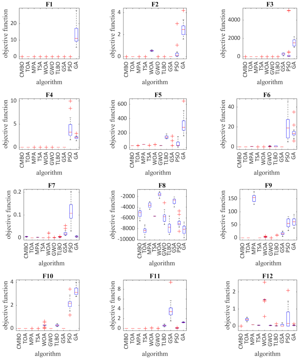
3.4. Statistical Analysis
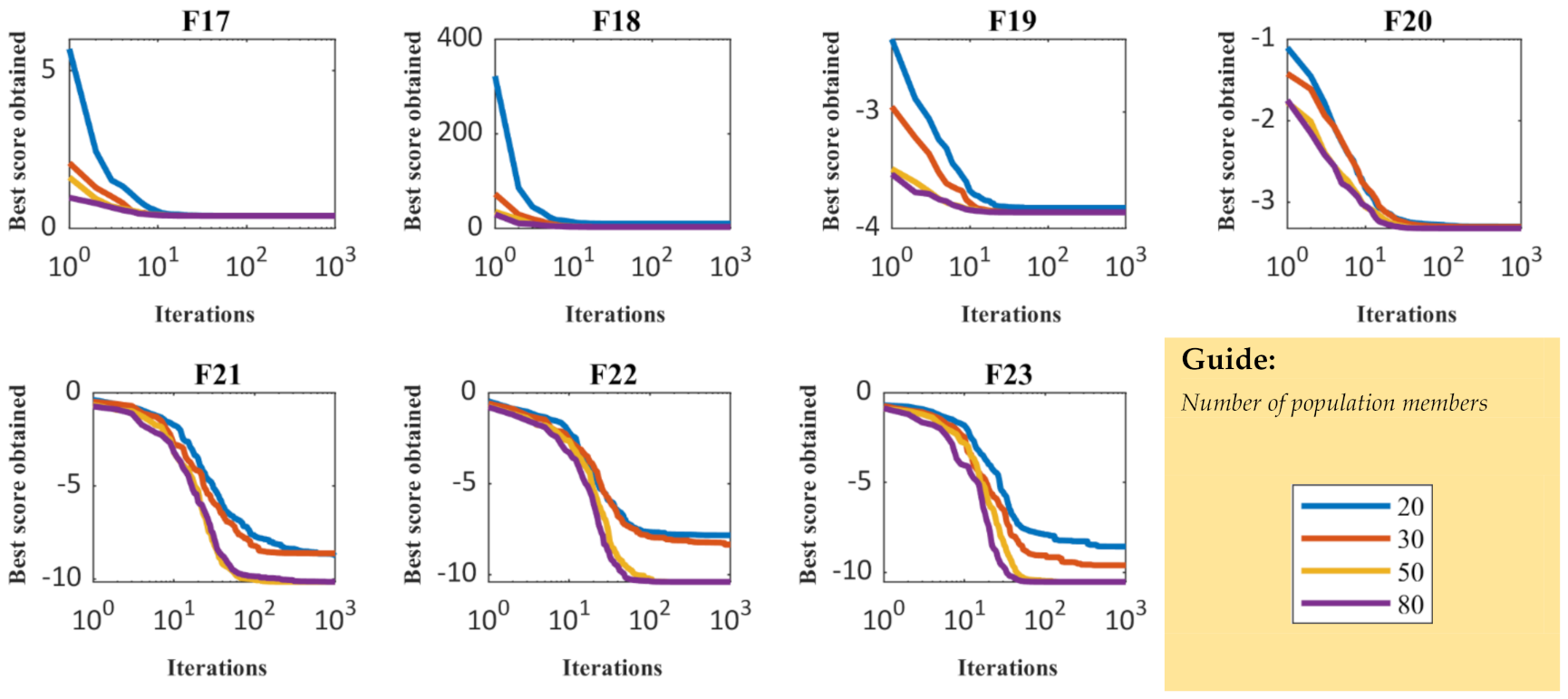
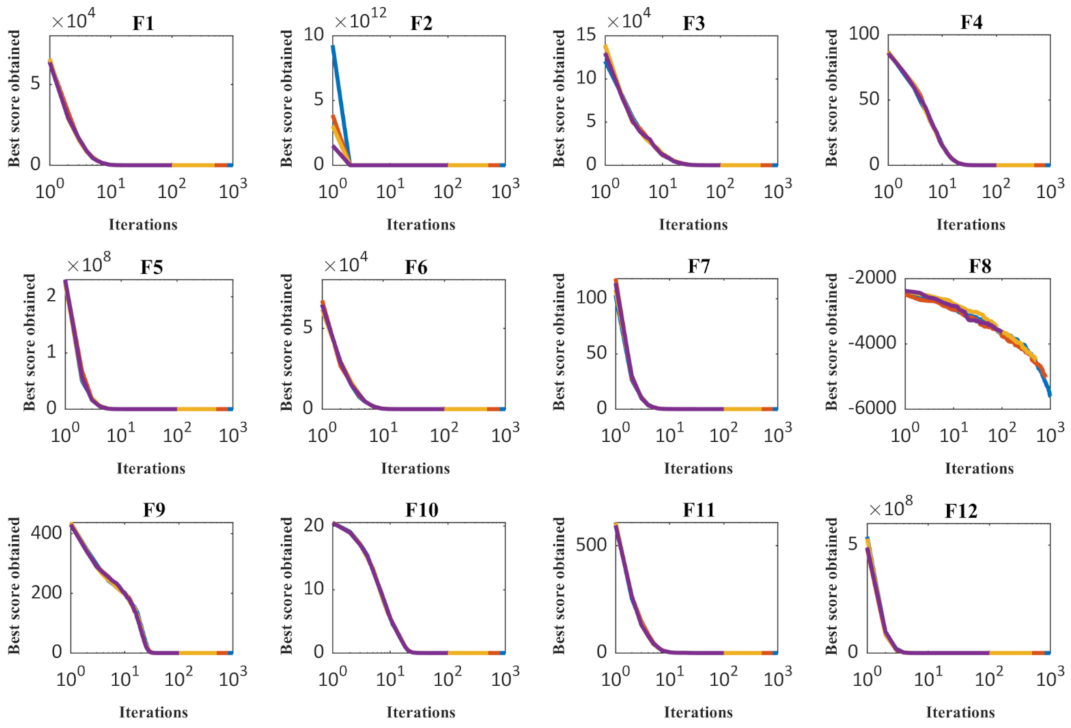
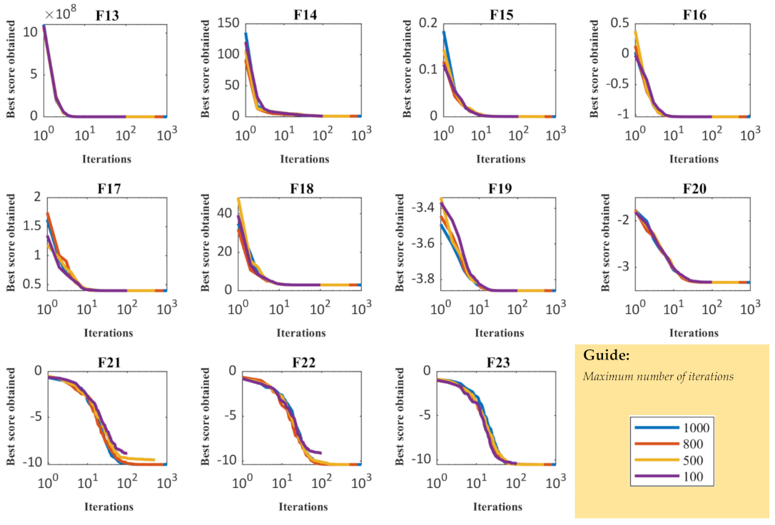
3.5. Sensitivity Analysis
4. Discussion
Execution Time Analysis
5. Conclusions and Feature Works
Author Contributions
Funding
Institutional Review Board Statement
Informed Consent Statement
Data Availability Statement
Acknowledgments
Conflicts of Interest
Appendix A

| Objective Function | Range | Dimensions | Fmin |
|---|---|---|---|
| 30 | 0 | ||
| 30 | 0 | ||
| 30 | 0 | ||
| 30 | 0 | ||
| 30 | 0 | ||
| 30 | 0 | ||
| 30 | 0 |
| Objective Function | Range | Dimensions | Fmin |
|---|---|---|---|
| 30 | −12,569 | ||
| 30 | 0 | ||
| 30 | 0 | ||
| 30 | 0 | ||
| 30 | 0 | ||
| 30 | 0 |
| Objective Function | Range | Dimensions | Fmin |
|---|---|---|---|
| 2 | 0.998 | ||
| 4 | 0.00030 | ||
| 2 | −1.0316 | ||
| [−5,10][0,15] | 2 | 0.398 | |
| 2 | 3 | ||
| 3 | −3.86 | ||
| 6 | −3.22 | ||
| 4 | −10.1532 | ||
| 4 | −10.4029 | ||
| 4 | −10.5364 |
References
- Dehghani, M.; Montazeri, Z.; Dehghani, A.; Ramirez-Mendoza, R.A.; Samet, H.; Guerrero, J.M.; Dhiman, G. MLO: Multi leader optimizer. Int. J. Intell. Eng. Syst. 2020, 13, 364–373. [Google Scholar] [CrossRef]
- Dhiman, G. SSC: A hybrid nature-inspired meta-heuristic optimization algorithm for engineering applications. Knowl. Based Syst. 2021, 222, 106926. [Google Scholar] [CrossRef]
- Sadeghi, A.; Doumari, S.A.; Dehghani, M.; Montazeri, Z.; Trojovský, P.; Ashtiani, H.J. A New “Good and Bad Groups-Based Optimizer” for Solving Various Optimization Problems. Appl. Sci. 2021, 11, 4382. [Google Scholar] [CrossRef]
- Cavazzuti, M. Deterministic Optimization. In Optimization Methods: From Theory to Design Scientific and Technological Aspects in Mechanics; Springer: Berlin/Heidelberg, Germany, 2013; pp. 77–102. [Google Scholar]
- Dhiman, G.; Kumar, V. Spotted hyena optimizer: A novel bio-inspired based metaheuristic technique for engineering applications. Adv. Eng. Softw. 2017, 114, 48–70. [Google Scholar] [CrossRef]
- Dorigo, M.; Birattari, M.; Stutzle, T. Ant colony optimization. IEEE Comput. Intell. Mag. 2006, 1, 28–39. [Google Scholar] [CrossRef] [Green Version]
- Goldberg, D.E.; Holland, J.H. Genetic Algorithms and Machine Learning. Mach. Learn. 1988, 3, 95–99. [Google Scholar] [CrossRef]
- Kennedy, J.; Eberhart, R. In Particle swarm optimization. In Proceedings of the ICNN’95—International Conference on Neural Networks, Perth, Australia, 27 November–1 December 1995; Volume 4, pp. 1942–1948. [Google Scholar]
- Rashedi, E.; Nezamabadi-Pour, H.; Saryazdi, S. GSA: A gravitational search algorithm. Inf. Sci. 2009, 179, 2232–2248. [Google Scholar] [CrossRef]
- Rao, R.V.; Savsani, V.J.; Vakharia, D.P. Teaching–learning-based optimization: A novel method for constrained mechanical design optimization problems. Comput. Aided Des. 2011, 43, 303–315. [Google Scholar] [CrossRef]
- Mirjalili, S.; Mirjalili, S.M.; Lewis, A. Grey wolf optimizer. Adv. Eng. Softw. 2014, 69, 46–61. [Google Scholar] [CrossRef] [Green Version]
- Mirjalili, S.; Lewis, A. The whale optimization algorithm. Adv. Eng. Softw. 2016, 95, 51–67. [Google Scholar] [CrossRef]
- Faramarzi, A.; Heidarinejad, M.; Mirjalili, S.; Gandomi, A.H. Marine Predators Algorithm: A nature-inspired metaheuristic. Expert Syst. Appl. 2020, 152, 113377. [Google Scholar] [CrossRef]
- Kaur, S.; Awasthi, L.K.; Sangal, A.L.; Dhiman, G. Tunicate Swarm Algorithm: A new bio-inspired based metaheuristic paradigm for global optimization. Eng. Appl. Artif. Intell. 2020, 90. [Google Scholar] [CrossRef]
- Dehghani, M.; Trojovský, P. Teamwork Optimization Algorithm: A New Optimization Approach for Function Minimization/Maximization. Sensors 2021, 21, 4567. [Google Scholar] [CrossRef]
- Yang, X.; Suash, D. Cuckoo Search via Lévy flights. In Proceedings of the 2009 World Congress on Nature and Biologically Inspired Computing (NaBIC), Coimbatore, India, 9–11 December 2009; pp. 210–214. [Google Scholar]
- Abualigah, L.; Yousri, D.; Elaziz, M.A.; Ewees, A.A.; Al-Qaness, M.A.; Gandomi, A.H. Aquila Optimizer: A novel meta-heuristic optimization algorithm. Comput. Ind. Eng. 2021, 157, 107250. [Google Scholar] [CrossRef]
- Yazdani, M.; Jolai, F. Lion Optimization Algorithm (LOA): A nature-inspired metaheuristic algorithm. J. Comput. Des. Eng. 2016, 3, 24–36. [Google Scholar] [CrossRef] [Green Version]
- Saremi, S.; Mirjalili, S.; Lewis, A. Grasshopper Optimisation Algorithm: Theory and application. Adv. Eng. Softw. 2017, 105, 30–47. [Google Scholar] [CrossRef] [Green Version]
- Dhiman, G.; Kumar, V. Emperor penguin optimizer: A bio-inspired algorithm for engineering problems. Knowl. Based Syst. 2018, 159, 20–50. [Google Scholar] [CrossRef]
- Chu, S.-C.; Tsai, P.-W.; Pan, J.-S. Cat swarm optimization. In Proceedings of the 9th Pacific Rim International Conference on Artificial Intelligence, Guilin, China, 7–11 August 2006; pp. 854–858. [Google Scholar]
- Kallioras, N.A.; Lagaros, N.D.; Avtzis, D.N. Pity beetle algorithm—A new metaheuristic inspired by the behavior of bark beetles. Adv. Eng. Softw. 2018, 121, 147–166. [Google Scholar] [CrossRef]
- Jahani, E.; Chizari, M. Tackling global optimization problems with a novel algorithm—Mouth Brooding Fish algorithm. Appl. Soft Comput. 2018, 62, 987–1002. [Google Scholar] [CrossRef]
- Shadravan, S.; Naji, H.R.; Bardsiri, V.K. The Sailfish Optimizer: A novel nature-inspired metaheuristic algorithm for solving constrained engineering optimization problems. Eng. Appl. Artif. Intell. 2019, 80, 20–34. [Google Scholar] [CrossRef]
- Dehghani, M.; Mardaneh, M.; Malik, O.P. FOA: ‘Following’ Optimization Algorithm for solving Power engineering optimization problems. J. Oper. Autom. Power Eng. 2020, 8, 57–64. [Google Scholar]
- Dehghani, M.; Montazeri, Z.; Dehghani, A.; Samet, H.; Sotelo, C.; Sotelo, D.; Ehsanifar, A.; Malik, O.P.; Guerrero, J.M.; Dhiman, G.; et al. DM: Dehghani Method for Modifying Optimization Algorithms. Appl. Sci. 2020, 10, 7683. [Google Scholar] [CrossRef]
- Storn, R.; Price, K.V. Differential Evolution—A Simple and Efficient Heuristic for global Optimization over Continuous Spaces. J. Glob. Optim. 1997, 11, 341–359. [Google Scholar] [CrossRef]
- Beyer, H.-G.; Schwefel, H.-P. Evolution strategies—A comprehensive introduction. Nat. Comput. 2002, 1, 3–52. [Google Scholar] [CrossRef]
- Simon, D. Biogeography-Based Optimization. IEEE Trans. Evol. Comput. 2008, 12, 702–713. [Google Scholar] [CrossRef] [Green Version]
- Huang, G. Artificial infectious disease optimization: A SEIQR epidemic dynamic model-based function optimization algorithm. Swarm Evol. Comput. 2016, 27, 31–67. [Google Scholar] [CrossRef] [PubMed]
- Labbi, Y.; Ben Attous, D.; Gabbar, H.A.; Mahdad, B.; Zidan, A. A new rooted tree optimization algorithm for economic dispatch with valve-point effect. Int. J. Electr. Power Energy Syst. 2016, 79, 298–311. [Google Scholar] [CrossRef]
- Baykasoğlu, A.; Akpinar, Ş. Weighted Superposition Attraction (WSA): A swarm intelligence algorithm for optimization problems—Part 1: Unconstrained optimization. Appl. Soft Comput. 2017, 56, 520–540. [Google Scholar] [CrossRef]
- Akyol, S.; Alatas, B. Plant intelligence based metaheuristic optimization algorithms. Artif. Intell. Rev. 2016, 47, 417–462. [Google Scholar] [CrossRef]
- Salmani, M.H.; Eshghi, K. A Metaheuristic Algorithm Based on Chemotherapy Science: CSA. J. Optim. 2017, 2017. [Google Scholar] [CrossRef]
- Cheraghalipour, A.; Hajiaghaei-Keshteli, M.; Paydar, M.M. Tree Growth Algorithm (TGA): A novel approach for solving optimization problems. Eng. Appl. Artif. Intell. 2018, 72, 393–414. [Google Scholar] [CrossRef]
- van Laarhoven, P.J.M.; Aarts, E.H.L. (Eds.) Simulated annealing. In Simulated Annealing: Theory and Applications; Springer: Dordrecht, The Netherland, 1987; pp. 7–15. [Google Scholar]
- Eskandar, H.; Sadollah, A.; Bahreininejad, A.; Hamdi, M. Water cycle algorithm—A novel metaheuristic optimization method for solving constrained engineering optimization problems. Comput. Struct. 2012, 110, 151–166. [Google Scholar] [CrossRef]
- Kaveh, A.; Bakhshpoori, T. Water Evaporation Optimization: A novel physically inspired optimization algorithm. Comput. Struct. 2016, 167, 69–85. [Google Scholar] [CrossRef]
- Muthiah-Nakarajan, V.; Noel, M.M. Galactic Swarm Optimization: A new global optimization metaheuristic inspired by galactic motion. Appl. Soft Comput. 2016, 38, 771–787. [Google Scholar] [CrossRef]
- Dehghani, M.; Montazeri, Z.; Dehghani, A.; Seifi, A. Spring search algorithm: A new meta-heuristic optimization algorithm inspired by Hooke’s law. In Proceedings of the 2017 IEEE 4th International Conference on Knowledge-Based Engineering and Innovation (KBEI), Tehran, Iran, 22 December 2017; pp. 210–214. [Google Scholar]
- Zhang, Q.; Wang, R.; Yang, J.; Ding, K.; Li, Y.; Hu, J. Collective decision optimization algorithm: A new heuristic optimization method. Neurocomputing 2017, 221, 123–137. [Google Scholar] [CrossRef]
- Vommi, V.B.; Vemula, R. A very optimistic method of minimization (VOMMI) for unconstrained problems. Inf. Sci. 2018, 454–455, 255–274. [Google Scholar] [CrossRef]
- Dehghani, M.; Samet, H. Momentum search algorithm: A new meta-heuristic optimization algorithm inspired by momentum conservation law. SN Appl. Sci. 2020, 2. [Google Scholar] [CrossRef]
- Hashim, F.A.; Hussain, K.; Houssein, E.H.; Mabrouk, M.S.; Al-Atabany, W. Archimedes optimization algorithm: A new metaheuristic algorithm for solving optimization problems. Appl. Intell. 2021, 51, 1531–1551. [Google Scholar] [CrossRef]
- Dehghani, M.; Montazeri, Z.; Malik, O.P. DGO: Dice game optimizer. GAZI Univ. J. Sci. 2019, 32, 871–882. [Google Scholar] [CrossRef] [Green Version]
- Dehghani, M.; Montazeri, Z.; Malik, O.P.; Dhiman, G.; Kumar, V. BOSA: Binary orientation search algorithm. Int. J. Innov. Technol. Explor. Eng. 2019, 9, 5306–5310. [Google Scholar]
- Dehghani, M.; Montazeri, Z.; Saremi, S.; Dehghani, A.; Malik, O.P.; Al-Haddad, K.; Guerrero, J. HOGO: Hide objects game optimization. Int. J. Intell. Eng. Syst. 2020, 13, 216–225. [Google Scholar] [CrossRef]
- Dehghani, M.; Mardaneh, M.; Guerrero, J.M.; Malik, O.; Kumar, V. Football game based optimization: An application to solve energy commitment problem. Int. J. Intell. Eng. Syst. 2020, 13, 514–523. [Google Scholar] [CrossRef]
- Dehghani, M.; Montazeri, Z.; Givi, H.; Guerrero, J.M.; Dhiman, G. Darts game optimizer: A new optimization technique based on darts game. Int. J. Intell. Eng. Syst. 2020, 13, 286–294. [Google Scholar] [CrossRef]
- Dehghani, M.; Montazeri, Z.; Malik, O.; Givi, H.; Guerrero, J. Shell Game Optimization: A Novel Game-Based Algorithm. Int. J. Intell. Eng. Syst. 2020, 13, 246–255. [Google Scholar] [CrossRef]
- Dehghani, M.; Montazeri, Z.; Hubálovský, Š. GMBO: Group Mean-Based Optimizer for Solving Various Optimization Problems. Mathematics 2021, 9, 1190. [Google Scholar] [CrossRef]


| Ref. | Algorithm | Main Idea (Inspiration Source) |
|---|---|---|
| [16] | Cuckoo Search | Behavior of cuckoo |
| [17] | Aquila Optimizer | Behavior of Aquila in nature during the process of catching the prey |
| [18] | Lion Optimization Algorithm | Behavior of lion |
| [19] | Grasshopper Optimization Algorithm | Grasshopper behavior |
| [20] | Emperor Penguin Optimizer | The behavior of emperor penguin |
| [21] | Cat Swarm Optimization Algorithm | Behaviors of cats |
| [22] | Pity Beetle Algorithm | Aggregation behavior, searching for nest and food |
| [23] | Mouth Brooding Fish | The behavior of mouthbrooding fish |
| [24] | Sailfish Optimizer | Group of hunting sailfish |
| [25] | Following Optimization Algorithm | Relationships between members and the leader of a community |
| [26] | Multi-Leader Optimizer | The presence of several leaders simultaneously for the population members |
| [27] | Differential Evolution | the natural phenomenon of evolution |
| [28] | Evolution Strategy | Darwinian evolution theory |
| [29] | Biogeography-Based Optimizer | Biogeographic concepts |
| [30] | Artificial Infectious Disease | SEIQR epidemic model |
| [31] | Rooted Tree Optimization | Plant roots movement looking for water |
| [32] | Weighted Superposition Attraction | Weighted superposition of active fields |
| [33] | Plant Intelligence | Plants nervous system |
| [34] | Chemotherapy Science | Chemotherapy method |
| [35] | Tree Growth Algorithm | Trees competition for acquiring light and foods |
| [36] | Simulated Annealing | Metal annealing process |
| [37] | Water Cycle Algorithms | Water cycle process and how rivers and streams flow to the sea in the real world |
| [38] | Water Evaporation Optimization | Evaporation of water molecules |
| [39] | Galactic Swarm Optimized Motion | The motion of stars, galaxies |
| [40] | Spring Search Algorithms | Hooke’s law |
| [41] | Collective Decision Optimization | The social behavior of human beings |
| [42] | Very Optimistic Method | Real-life practices of successful persons |
| [43] | Momentum Search Algorithm | Momentum law and Newton’s laws of motion |
| [44] | Archimedes Optimization Algorithm | Law of physics Archimedes’ Principle which imitates the principle of buoyant force exerted upward on an object |
| [45] | Dice Game Optimizer | Rules governing the game of dice and the impact of players on each other |
| [46] | Orientation Search Algorithm | Game of orientation, in which players move in the direction of a referee |
| [47] | Hide Objects Game Optimization | Behavior and movements of players to find a hidden object |
| [48] | Football Game Based Optimization | Simulation of behavior of clubs in football league. |
| [49] | Darts Game Optimizer | Rules of the Darts game |
| [50] | Shell Game Optimization | Rules of the shell game |
| Step 1 | Step 2 | Step 3 | Step 4 | Step 5 | Step 6 | |||||||||
|---|---|---|---|---|---|---|---|---|---|---|---|---|---|---|
| X | F(X) | XS | FS(X) | Cats | Mice | C | FC | M | Fm | |||||
| x1 | x2 | c1 | c2 | m1 | m2 | |||||||||
| X1 | 69.00641 | −74.5553 | 10,320.38 | −36.7889 | 19.51363 | 1734.208 | M1 | −36.7889 | 19.51363 | 1734.208 | ||||
| X2 | 18.96709 | −45.9773 | 2473.659 | 18.96709 | −45.9773 | 2473.659 | M2 | 18.96709 | −45.9773 | 2473.659 | ||||
| X3 | 99.35621 | −34.7797 | 11,081.28 | 46.22603 | 18.41816 | 2476.074 | M3 | −12.7845 | 3.444065 | 175.3053 | ||||
| X4 | −36.7889 | 19.51363 | 1734.208 | 41.24409 | −45.8968 | 3807.588 | M4 | 32.03547 | −45.8968 | 3132.784 | ||||
| X5 | 46.22603 | 18.41816 | 2476.074 | 68.51469 | −19.8287 | 5087.439 | M5 | −3.47199 | −20.895 | 448.6563 | ||||
| X6 | −91.4795 | 76.26784 | 14,185.29 | 57.48351 | 58.62186 | 6740.877 | C1 | 52.12189 | −42.9835 | 4564.272 | ||||
| X7 | 68.51469 | −19.8287 | 5087.439 | 69.00641 | −74.5553 | 10,320.38 | C2 | −24.7895 | −40.9822 | 2294.059 | ||||
| X8 | −64.1203 | −80.2158 | 10,545.99 | −64.1203 | −80.2158 | 10,545.99 | C3 | −51.4096 | −50.6034 | 5203.653 | ||||
| X9 | 41.24409 | −45.8968 | 3807.588 | 99.35621 | −34.7797 | 11,081.28 | C4 | 87.51208 | −30.541 | 8591.116 | ||||
| X10 | 57.48351 | 58.62186 | 6740.877 | −91.4795 | 76.26784 | 14,185.29 | C5 | −16.7554 | 52.75574 | 3063.913 | ||||
| Full implementation | ||||||||||||||
| Best Solution: x1 = 3.51 × 10⁻¹², x2 = 6.73 × 10⁻¹² and F(X) = 5.7626 × 10⁻²³ | ||||||||||||||
| Algorithm | Parameter | Value |
|---|---|---|
| GA | ||
| Type | Real coded | |
| Selection | Roulette wheel (Proportionate) | |
| Crossover | Whole arithmetic (Probability = 0.8, ) | |
| Mutation | Gaussian (Probability = 0.05) | |
| PSO | ||
| Topology | Fully connected | |
| Cognitive and social constant | (C1, C2) = (2, 2) | |
| Inertia weight | Linear reduction from 0.9 to 0.1 | |
| Velocity limit | 10% of dimension range | |
| GSA | ||
| Alpha, G0, Rnorm, Rpower | 20, 100, 2, 1 | |
| TLBO | ||
| TF: teaching factor | round | |
| random number | rand is a random number in the range | |
| GWO | ||
| Convergence parameter (a) | a: Linear reduction from 2 to 0. | |
| WOA | ||
| Convergence parameter (a) | a: Linear reduction from 2 to 0. | |
| r is a random vector in | ||
| l is a random number in | ||
| TSA | ||
| Pmin and Pmax | 1, 4 | |
| C1, C2, C3 | random numbers, which lie in the range | |
| MPA | ||
| Constant number | p 0.5 | |
| Random vector | R is a vector of uniform random numbers in the range | |
| Fish Aggregating Devices (FADs) | FADs 0.2 | |
| Binary vector | U 0 or 1 | |
| TOA | ||
| Update index | round | |
| r | r is a uniform random number in the range | |
| CMBO | TOA | MPA | TSA | WOA | GWO | TLBO | GSA | PSO | GA | ||
|---|---|---|---|---|---|---|---|---|---|---|---|
| F1 | ave | 2.69 × 10−236 | 0 | 3.2715 × 10⁻²¹ | 7.71 × 10−38 | 2.1741 × 10⁻⁹ | 1.09 × 10−58 | 8.3373 × 10−60 | 2.0255 × 10⁻¹⁷ | 1.7740 × 10⁻⁵ | 13.2405 |
| std | 0 | 0 | 4.6153 × 10⁻²¹ | 7.00 × 10⁻²¹ | 7.3985 × 10⁻²⁵ | 5.1413 × 10−74 | 4.9436 × 10−76 | 1.1369 × 10⁻³² | 6.4396 × 10⁻²¹ | 4.7664 × 10⁻¹⁵ | |
| F2 | ave | 6.88 × 10−121 | 0 | 1.57 × 10⁻¹² | 8.48 × 10−39 | 0.5462 | 1.2952 × 10⁻³⁴ | 7.1704 × 10⁻³⁵ | 2.3702 × 10⁻⁸ | 0.3411 | 2.4794 |
| std | 2.46 × 10−135 | 0 | 1.42 × 10⁻¹² | 5.92 × 10−41 | 1.7377 × 10⁻¹⁶ | 1.9127 × 10−50 | 6.6936 × 10−50 | 5.1789 × 10⁻²⁴ | 7.4476 × 10⁻¹⁷ | 2.2342 × 10⁻¹⁵ | |
| F3 | ave | 2.44 × 10−60 | 0 | 0.0864 | 1.15 × 10⁻²¹ | 1.7634 × 10⁻⁸ | 7.4091 × 10⁻¹⁵ | 2.7531 × 10⁻¹⁵ | 279.3439 | 589.492 | 1536.8963 |
| std | 1.82 × 10−67 | 0 | 0.1444 | 6.70 × 10⁻²¹ | 1.0357 × 10⁻²³ | 5.6446 × 10⁻³⁰ | 2.6459 × 10⁻³¹ | 1.2075 × 10⁻¹³ | 7.1179 × 10⁻¹³ | 6.6095 × 10⁻¹³ | |
| F4 | ave | 1.04 × 10−93 | 0 | 2.6 × 10⁻⁸ | 1.33 × 10⁻²³ | 2.9009 × 10⁻⁵ | 1.2599 × 10⁻¹⁴ | 9.4199 × 10⁻¹⁵ | 3.2547 × 10⁻⁹ | 3.9634 | 2.0942 |
| std | 2.09 × 10−108 | 0 | 9.25 × 10⁻⁹ | 1.15 × 10⁻²² | 1.2121 × 10⁻²⁰ | 1.0583 × 10⁻²⁹ | 2.1167 × 10⁻³⁰ | 2.0346 × 10⁻²⁴ | 1.9860 × 10⁻¹⁶ | 2.2342 × 10⁻¹⁵ | |
| F5 | ave | 24.87011 | 26.2476 | 46.049 | 28.8615 | 41.7767 | 26.8607 | 146.4564 | 36.10695 | 50.26245 | 310.4273 |
| std | 1.91 × 10⁻¹⁴ | 3.26 × 10⁻¹⁴ | 0.4219 | 4.76 × 10⁻³ | 2.5421 × 10⁻¹⁴ | 0 | 1.9065 × 10⁻¹⁴ | 3.0982 × 10⁻¹⁴ | 1.5888 × 10⁻¹⁴ | 2.0972 × 10⁻¹³ | |
| F6 | ave | 0 | 0 | 0.398 | 7.10 × 10⁻²¹ | 1.6085 × 10⁻⁹ | 0.6423 | 0.4435 | 0 | 20.25 | 14.55 |
| std | 0 | 0 | 0.1914 | 1.12 × 10⁻²⁵ | 4.6240 × 10⁻²⁵ | 6.2063 × 10⁻¹⁷ | 4.2203 × 10⁻¹⁶ | 0 | 1.2564 | 3.1776 × 10⁻¹⁵ | |
| F7 | ave | 0.002709 | 9.92 × 10−06 | 0.0018 | 3.72 × 10⁻⁴ | 0.0205 | 0.0008 | 0.0017 | 0.0206 | 0.1134 | 5.6799 × 10⁻³ |
| std | 1.94 × 10⁻¹⁹ | 1.74 × 10⁻²⁰ | 0.001 | 5.09 × 10⁻⁵ | 1.5515 × 10⁻¹⁸ | 7.2730 × 10⁻²⁰ | 3.87896 × 10⁻¹⁹ | 2.7152 × 10⁻¹⁸ | 4.3444 × 10⁻¹⁷ | 7.7579 × 10⁻¹⁹ | |
| CMBO | TOA | MPA | TSA | WOA | GWO | TLBO | GSA | PSO | GA | ||
|---|---|---|---|---|---|---|---|---|---|---|---|
| F8 | ave | −6561.15 | −9631.41 | −3594.1632 | −5740.3388 | −1663.9782 | −5885.1172 | −7408.6107 | −2849.0724 | −6908.6558 | −8184.4142 |
| std | 1.83 × 10⁻¹² | 3.86 × 10⁻¹² | 811.32651 | 41.5 | 716.3492 | 467.5138 | 513.5784 | 264.3516 | 625.6248 | 833.2165 | |
| F9 | ave | 0 | 0 | 140.1238 | 5.70 × 10⁻³ | 4.2011 | 8.5265 × 10⁻¹⁵ | 10.2485 | 16.2675 | 57.0613 | 62.4114 |
| std | 0 | 0 | 26.3124 | 1.46 × 10⁻³ | 4.3692 × 10⁻¹⁵ | 5.6446 × 10⁻³⁰ | 5.5608 × 10⁻¹⁵ | 3.1776 × 10⁻¹⁵ | 6.3552 × 10⁻¹⁵ | 2.5421 × 10⁻¹⁴ | |
| F10 | ave | 4.44 × 10⁻¹⁵ | 8.88 × 10⁻¹⁶ | 9.6987 × 10⁻¹² | 9.80 × 10⁻¹⁴ | 0.3293 | 1.7053 × 10⁻¹⁴ | 0.2757 | 3.5673 × 10⁻⁹ | 2.1546 | 3.2218 |
| std | 0 | 0 | 6.1325 × 10⁻¹² | 4.51 × 10⁻¹² | 1.9860 × 10⁻¹⁶ | 2.7517 × 10⁻²⁹ | 2.5641 × 10⁻¹⁵ | 3.6992 × 10⁻²⁵ | 7.9441 × 10⁻¹⁶ | 5.1636 × 10⁻¹⁵ | |
| F11 | ave | 0 | 0 | 0 | 1.00 × 10⁻⁷ | 0.1189 | 0.0037 | 0.6082 | 3.7375 | 0.0462 | 1.2302 |
| std | 0 | 0 | 0 | 7.46 × 10⁻⁷ | 8.9991 × 10⁻¹⁷ | 1.2606 × 10⁻¹⁸ | 1.9860 × 10⁻¹⁶ | 2.7804 × 10⁻¹⁵ | 3.1031 × 10⁻¹⁸ | 8.4406 × 10⁻¹⁶ | |
| F12 | ave | 1.10 × 10−08 | 0.2463 | 0.0851 | 0.0368 | 1.7414 | 0.0372 | 0.0203 | 0.0362 | 0.4806 | 0.047 |
| std | 1.66 × 10⁻²² | 7.45 × 10⁻¹⁷ | 0.0052 | 1.5461 × 10⁻² | 8.1347 × 10⁻¹² | 4.3444 × 10⁻¹⁷ | 7.7579 × 10⁻¹⁹ | 6.2063 × 10⁻¹⁸ | 1.8619 × 10⁻¹⁶ | 4.6547 × 10⁻¹⁸ | |
| F13 | ave | 1.78 × 10−07 | 1.25 | 0.4901 | 2.9575 | 0.3456 | 0.5763 | 0.3293 | 0.002 | 0.5084 | 1.2085 |
| std | 3.10 × 10⁻¹⁸ | 4.47 × 10⁻¹⁶ | 0.1932 | 1.5682 × 10⁻¹² | 3.25391 × 10⁻¹² | 2.4825 × 10⁻¹⁵ | 2.1101 × 10⁻¹⁴ | 4.2617 × 10⁻¹⁴ | 4.9650 × 10⁻¹⁷ | 3.2272 × 10⁻¹⁶ | |
| CMBO | TOA | MPA | TSA | WOA | GWO | TLBO | GSA | PSO | GA | ||
|---|---|---|---|---|---|---|---|---|---|---|---|
| F14 | ave | 0.998 | 0.9980 | 0.998 | 1.9923 | 0.998 | 3.7408 | 2.2721 | 3.5913 | 2.1735 | 0.9986 |
| std | 0 | 4.72 × 10⁻¹⁶ | 4.2735 × 10⁻¹⁶ | 2.6548 × 10⁻⁷ | 9.4336 × 10⁻¹⁶ | 6.4545 × 10⁻¹⁵ | 1.9860 × 10⁻¹⁶ | 7.9441 × 10⁻¹⁶ | 7.9441 × 10⁻¹⁶ | 1.5640 × 10⁻¹⁵ | |
| F15 | ave | 0.000307 | 0.000307 | 0.003 | 0.0004 | 0.0049 | 0.0063 | 0.0033 | 0.0024 | 0.0535 | 5.3952 × 10⁻² |
| std | 1.21 × 10⁻²⁰ | 1.16 × 10⁻¹⁸ | 4.0951 × 10⁻¹⁵ | 9.0125 × 10⁻⁴ | 3.4910 × 10⁻¹⁸ | 1.1636 × 10⁻¹⁸ | 1.2218 × 10⁻¹⁷ | 2.9092 × 10⁻¹⁹ | 3.8789 × 10⁻¹⁹ | 7.0791 × 10⁻¹⁸ | |
| F16 | ave | −1.03163 | −1.0316 | −1.0316 | −1.0316 | −1.0316 | −1.0316 | −1.0316 | −1.0316 | −1.0316 | −1.0316 |
| std | 1.47 × 10⁻¹⁶ | 1.99 × 10⁻¹⁶ | 4.4652 × 10⁻¹⁶ | 2.6514 × 10⁻¹⁶ | 9.9301 × 10⁻¹⁶ | 3.9720 × 10⁻¹⁶ | 1.4398 × 10⁻¹⁵ | 5.9580 × 10⁻¹⁶ | 3.4755 × 10⁻¹⁶ | 7.9441 × 10⁻¹⁶ | |
| F17 | ave | 0.3978 | 0.3978 | 0.3979 | 0.3991 | 0.4047 | 0.3978 | 0.3978 | 0.3978 | 0.7854 | 0.4369 |
| std | 0 | 9.93 × 10⁻¹⁷ | 9.1235 × 10⁻¹⁵ | 2.1596 × 10⁻¹⁶ | 2.4825 × 10⁻¹⁷ | 8.6888 × 10⁻¹⁷ | 7.4476 × 10⁻¹⁷ | 9.9301 × 10⁻¹⁷ | 4.9650 × 10⁻¹⁷ | 4.9650 × 10⁻¹⁷ | |
| F18 | ave | 3 | 3 | 3 | 3 | 3 | 3 | 3.0009 | 3 | 3 | 4.3592 |
| std | 0 | 0 | 1.9584 × 10⁻¹⁵ | 2.6528 × 10⁻¹⁵ | 5.6984 × 10⁻¹⁵ | 2.0853 × 10⁻¹⁵ | 1.5888 × 10⁻¹⁵ | 6.9511 × 10⁻¹⁶ | 3.6741 × 10⁻¹⁵ | 5.9580 × 10⁻¹⁶ | |
| F19 | ave | −3.86278 | −3.86278 | −3.8627 | −3.8066 | −3.8627 | −3.8621 | −3.8609 | −3.8627 | −3.8627 | −3.85434 |
| std | 1.83 × 10⁻¹⁶ | 2.68 × 10⁻¹⁶ | 4.2428 × 10⁻¹⁵ | 2.6357 × 10⁻¹⁵ | 3.1916 × 10⁻¹⁵ | 2.4825 × 10⁻¹⁵ | 7.3483 × 10⁻¹⁵ | 8.3413 × 10⁻¹⁵ | 8.9371 × 10⁻¹⁵ | 9.9301 × 10⁻¹⁷ | |
| F20 | ave | −3.322 | −3.322 | −3.3211 | −3.3206 | −3.2424 | −3.2523 | −3.2014 | −3.0396 | −3.2619 | −2.8239 |
| std | 1.59 × 10⁻¹⁶ | 1.69 × 10⁻¹⁵ | 1.1421 × 10⁻¹¹ | 5.6918 × 10⁻¹⁵ | 7.9441 × 10⁻¹⁶ | 2.1846 × 10⁻¹⁵ | 1.7874 × 10⁻¹⁵ | 2.1846 × 10⁻¹⁴ | 2.9790 × 10⁻¹⁶ | 3.97205 × 10⁻¹⁶ | |
| F21 | ave | −10.1532 | −10.1532 | −10.1532 | −5.5021 | −7.4016 | −9.6452 | −9.1746 | −5.1486 | −5.3891 | −4.3040 |
| std | 1.15 × 10⁻¹⁶ | 1.39 × 10⁻¹⁵ | 2.5361 × 10⁻¹¹ | 5.4615 × 10⁻¹³ | 2.3819 × 10⁻¹¹ | 6.5538 × 10⁻¹⁵ | 8.5399 × 10⁻¹⁵ | 2.9790 × 10⁻¹⁶ | 1.4895 × 10⁻¹⁵ | 1.5888 × 10⁻¹⁵ | |
| F22 | ave | −10.4029 | −10.4029 | −10.4029 | −5.0625 | −8.8165 | −10.4025 | −10.0389 | −9.0239 | −7.6323 | −5.1174 |
| std | 1.39 × 10⁻¹⁶ | 3.18 × 10⁻¹⁵ | 2.8154 × 10⁻¹¹ | 8.4637 × 10⁻¹⁴ | 6.7524 × 10⁻¹⁵ | 1.9860 × 10⁻¹⁵ | 1.5292 × 10⁻¹⁴ | 1.6484 × 10⁻¹² | 1.5888 × 10⁻¹⁵ | 1.2909 × 10⁻¹⁵ | |
| F23 | ave | −10.5364 | −10.5364 | −10.5364 | −10.3613 | −10.0003 | −10.1302 | −9.2905 | −8.9045 | −6.1648 | −6.5621 |
| std | 1.35 × 10⁻¹⁶ | 7.94 × 10⁻¹⁶ | 3.9861 × 10⁻¹¹ | 7.6492 × 10⁻¹² | 9.1357 × 10⁻¹⁵ | 4.5678 × 10⁻¹⁵ | 1.1916 × 10⁻¹⁵ | 7.1497 × 10⁻¹⁴ | 2.7804 × 10⁻¹⁵ | 3.8727 × 10⁻¹⁵ | |
| Compared Algorithms | Unimodal | High-Dimensional Multi Modal | Fixed-Dimensional Multi Modal |
|---|---|---|---|
| CMBO vs. TOA | 0.4375 | 0.4375 | 0.625 |
| CMBO vs. TSA | 0.109375 | 0.0625 | 0.0625 |
| CMBO vs. MPA | 0.015625 | 0.03125 | 0.003906 |
| CMBO vs. WOA | 0.015625 | 0.03125 | 0.007813 |
| CMBO vs. GWO | 0.15625 | 0.03125 | 0.011719 |
| CMBO vs. TLBO | 0.15625 | 0.4375 | 0.005859 |
| CMBO vs. GSA | 0.03125 | 0.03125 | 0.019531 |
| CMBO vs. PSO | 0.015625 | 0.4375 | 0.003906 |
| CMBO vs. GA | 0.015625 | 0.4375 | 0.001953 |
| Objective Functions | Number of Population Members | |||
|---|---|---|---|---|
| 20 | 30 | 50 | 80 | |
| F1 | 3.7 × 10−201 | 1.4 × 10−214 | 2.7 × 10−236 | 1.1 × 10−243 |
| F2 | 5.4 × 10−137 | 1.4 × 10−126 | 6.9 × 10−121 | 4.3 × 10−119 |
| F3 | 8.69 × 10−74 | 8.34 × 10−60 | 2.44 × 10−60 | 2.42 × 10−57 |
| F4 | 5.5 × 10−108 | 1.23 × 10−98 | 1.04 × 10−93 | 4.96 × 10−92 |
| F5 | 26.86162 | 25.87908 | 24.87011 | 24.58636 |
| F6 | 0 | 0 | 0 | 0 |
| F7 | 0.008517 | 0.006639 | 0.002709 | 0.001691 |
| F8 | −4696 | −7900.45 | −6561.15 | −7142.03 |
| F9 | 0 | 0 | 0 | 0 |
| F10 | 4.44 × 10⁻¹⁵ | 4.44 × 10⁻¹⁵ | 4.44 × 10⁻¹⁵ | 4.44 × 10⁻¹⁵ |
| F11 | 0 | 0 | 0 | 0 |
| F12 | 0.038614 | 0.003171 | 1.1 × 10−08 | 1.36 × 10−09 |
| F13 | 1.281798 | 0.305144 | 1.78 × 10−07 | 5.22 × 10−09 |
| F14 | 1.593234 | 1.196414 | 0.998 | 0.998004 |
| F15 | 0.000418 | 0.000311 | 0.000307 | 0.000307 |
| F16 | −1.03163 | −1.03163 | −1.03163 | −1.03163 |
| F17 | 0.397887 | 0.397887 | 0.3978 | 0.397887 |
| F18 | 9.75 | 3 | 3 | 3 |
| F19 | −3.82413 | −3.86278 | −3.86278 | −3.86278 |
| F20 | −3.3005 | −3.30416 | −3.322 | −3.322 |
| F21 | −8.71417 | −8.61749 | −10.1532 | −10.1532 |
| F22 | −7.84302 | −8.35605 | −10.4029 | −10.4029 |
| F23 | −8.57191 | −9.61404 | −10.5364 | −10.5364 |
| Objective Functions | Maximum number of iterations | |||
|---|---|---|---|---|
| 100 | 500 | 800 | 1000 | |
| F1 | 9.54 × 10⁻²⁰ | 6.7 × 10−115 | 9.3 × 10−187 | 2.7 × 10−236 |
| F2 | 9.48 × 10⁻¹¹ | 3.22 × 10−59 | 1.47 × 10−95 | 6.9 × 10−121 |
| F3 | 0.047734 | 7.69 × 10⁻²⁴ | 7.75 × 10−41 | 2.44 × 10−60 |
| F4 | 5.41 × 10−08 | 1.27 × 10−45 | 8.96 × 10−74 | 1.04 × 10−93 |
| F5 | 27.78238 | 26.04638 | 25.62131 | 24.87011 |
| F6 | 0 | 0 | 0 | 0 |
| F7 | 0.012014 | 0.005967 | 0.005116 | 0.002709 |
| F8 | −3642.94 | −4496.48 | −5014.61 | −6561.15 |
| F9 | 0 | 0 | 0 | 0 |
| F10 | 7.19 × 10⁻¹¹ | 4.44 × 10⁻¹⁵ | 4.44 × 10⁻¹⁵ | 4.44 × 10⁻¹⁵ |
| F11 | 0 | 0 | 0 | 0 |
| F12 | 0.023937 | 0.000129 | 1.23 × 10−05 | 1.1 × 10−08 |
| F13 | 0.324195 | 0.030145 | 0.016247 | 1.78 × 10−07 |
| F14 | 1.096872 | 0.998004 | 0.998004 | 0.998 |
| F15 | 0.000529 | 0.000341 | 0.000308 | 0.000307 |
| F16 | −1.03163 | −1.03163 | −1.03163 | −1.03163 |
| F17 | 0.397887 | 0.397887 | 0.397887 | 0.3978 |
| F18 | 3 | 3 | 3 | 3 |
| F19 | −3.86278 | −3.86278 | −3.86278 | −3.86278 |
| F20 | −3.31584 | −3.32199 | −3.322 | −3.322 |
| F21 | −8.93555 | −9.64077 | −10.1532 | −10.1532 |
| F22 | −9.13251 | −10.4027 | −10.4029 | −10.4029 |
| F23 | −10.4926 | −10.5364 | −10.5362 | −10.5364 |
| CMBO | TOA | MPA | TSA | WOA | GWO | TLBO | GSA | PSO | GA | ||
|---|---|---|---|---|---|---|---|---|---|---|---|
| F1 | ave_time | 2.06327 | 2.288047 | 2.828934 | 2.27456 | 2.856446 | 3.142379 | 3.662429 | 9.024897 | 3.685416 | 3.876233 |
| std_time | 0.008802 | 0.103601 | 0.021766 | 0.00882 | 0.039718 | 0.01458 | 0.008365 | 0.110843 | 0.01622 | 0.044052 | |
| F2 | ave_time | 2.149418 | 2.33419 | 2.222183 | 2.496359 | 3.143495 | 3.000322 | 3.747463 | 9.602311 | 3.425936 | 3.34707 |
| std_time | 0.009976 | 0.05675 | 0.00619 | 0.004159 | 0.012551 | 0.001226 | 0.00205 | 0.029098 | 0.001869 | 0.001112 | |
| F3 | ave_time | 3.759693 | 6.014573 | 6.474818 | 5.805883 | 10.96679 | 6.132736 | 13.31042 | 11.65223 | 14.68167 | 12.16981 |
| std_time | 0.049343 | 0.184878 | 0.056553 | 0.003913 | 0.020291 | 0.002126 | 0.005486 | 0.05522 | 0.023614 | 0.063015 | |
| F4 | ave_time | 2.095707 | 2.303496 | 2.830211 | 2.429061 | 2.82791 | 2.884421 | 3.475663 | 9.399065 | 3.298336 | 3.218456 |
| std_time | 0.000425 | 0.058168 | 0.006382 | 0.001313 | 0.002522 | 0.000774 | 0.000146 | 0.095684 | 0.002026 | 0.001128 | |
| F5 | ave_time | 2.319993 | 2.668194 | 3.271111 | 2.837473 | 4.076267 | 3.362668 | 4.743216 | 9.85618 | 4.510391 | 4.74454 |
| std_time | 0.001194 | 0.098008 | 0.020855 | 0.001889 | 0.004884 | 0.0012 | 0.013286 | 0.000635 | 0.004473 | 0.015477 | |
| F6 | ave_time | 2.051842 | 2.142897 | 2.778443 | 2.388851 | 2.636699 | 2.884786 | 3.543828 | 9.739783 | 2.826627 | 3.964025 |
| std_time | 0.000734 | 0.053895 | 0.002564 | 0.000531 | 0.000103 | 0.000545 | 0.003082 | 0.081756 | 0.00079 | 0.002177 | |
| F7 | ave_time | 2.799308 | 3.426696 | 5.361778 | 4.208485 | 7.73167 | 4.624996 | 9.5011 | 11.0389 | 10.25112 | 8.948355 |
| std_time | 0.000298 | 0.138022 | 0.010684 | 0.001381 | 0.013762 | 0.000748 | 0.01131 | 0.002795 | 0.062275 | 0.003807 | |
| F8 | ave_time | 2.368102 | 2.787053 | 3.54212 | 3.038116 | 4.470513 | 3.45166 | 5.934958 | 10.15033 | 6.189501 | 5.35854 |
| std_time | 0.001774 | 0.146471 | 0.028588 | 0.001872 | 0.008998 | 0.000947 | 0.024404 | 0.002614 | 0.027143 | 0.006958 | |
| F9 | ave_time | 2.105224 | 2.141418 | 3.207098 | 2.70311 | 2.998242 | 2.962939 | 5.075711 | 10.07901 | 4.697519 | 4.632448 |
| std_time | 0.000457 | 0.022495 | 0.00947 | 0.000574 | 0.001451 | 0.001075 | 0.007871 | 0.034299 | 0.006383 | 0.001877 | |
| F10 | ave_time | 2.119633 | 2.213827 | 3.199752 | 2.685157 | 3.250468 | 2.951537 | 4.663569 | 9.862325 | 4.465213 | 4.851987 |
| std_time | 0.000675 | 0.106657 | 0.008234 | 0.001502 | 0.002534 | 0.000494 | 0.002845 | 0.030374 | 0.003311 | 0.000453 | |
| F11 | ave_time | 2.382237 | 2.702994 | 3.627042 | 3.029926 | 4.341168 | 3.544234 | 5.783952 | 10.09065 | 5.962496 | 5.935665 |
| std_time | 0.000521 | 0.090901 | 0.002333 | 0.006447 | 0.004761 | 0.011232 | 0.004814 | 0.001281 | 0.004878 | 0.010718 | |
| F12 | ave_time | 4.689757 | 6.401408 | 9.786492 | 7.746796 | 16.08114 | 8.081277 | 22.27949 | 13.02264 | 23.24494 | 18.18917 |
| std_time | 0.000582 | 0.136896 | 0.121341 | 0.003636 | 0.010787 | 0.005813 | 0.145335 | 0.001683 | 0.143479 | 0.016131 | |
| F13 | ave_time | 4.683313 | 6.317049 | 9.715068 | 7.882488 | 16.03426 | 8.216492 | 21.93277 | 12.87604 | 22.93827 | 17.26237 |
| std_time | 0.00164 | 0.142056 | 0.059173 | 0.015565 | 0.009175 | 0.040121 | 0.238577 | 0.080775 | 0.040952 | 0.026452 | |
| F14 | ave_time | 6.77659 | 11.05703 | 10.17388 | 11.25044 | 28.35404 | 10.67249 | 38.58243 | 10.43203 | 42.03153 | 31.15071 |
| std_time | 0.024394 | 0.495939 | 0.132818 | 0.007729 | 0.043197 | 0.004033 | 0.463309 | 0.00956 | 0.793664 | 0.187898 | |
| F15 | ave_time | 1.162517 | 2.036434 | 1.674953 | 1.143977 | 2.66252 | 1.168071 | 4.228257 | 4.381512 | 2.407291 | 3.348114 |
| std_time | 0.0006 | 0.076443 | 0.004268 | 0.001227 | 0.003729 | 0.000474 | 0.004635 | 0.000891 | 0.003895 | 0.000252 | |
| F16 | ave_time | 0.981154 | 1.965747 | 1.553408 | 1.014295 | 2.554895 | 0.98797 | 4.155264 | 3.895143 | 2.183457 | 3.277226 |
| std_time | 0.000487 | 0.097936 | 0.013704 | 0.001489 | 0.002058 | 0.000326 | 0.002632 | 0.006833 | 0.000941 | 0.000117 | |
| F17 | ave_time | 0.976854 | 1.818405 | 1.235874 | 0.86938 | 2.127932 | 0.865444 | 3.596898 | 3.391429 | 1.754779 | 2.926444 |
| std_time | 0.025755 | 0.076691 | 0.005655 | 0.000666 | 0.001913 | 0.000584 | 0.005077 | 0.002162 | 0.001703 | 0.000751 | |
| F18 | ave_time | 0.895712 | 1.828383 | 1.161598 | 0.778106 | 1.943841 | 0.827821 | 3.474254 | 3.32534 | 1.553584 | 3.013364 |
| std_time | 0.000171 | 0.115063 | 0.000996 | 5.56E-05 | 0.000193 | 0.000381 | 0.004198 | 0.007157 | 0.002831 | 0.002876 | |
| F19 | ave_time | 1.15748 | 2.291343 | 1.500319 | 1.165046 | 2.852 | 1.19711 | 4.232431 | 3.811885 | 2.8576 | 3.788615 |
| std_time | 0.002134 | 0.265954 | 0.00141 | 0.000364 | 0.00364 | 0.000711 | 0.007588 | 0.009134 | 0.009284 | 0.000403 | |
| F20 | ave_time | 1.282607 | 2.124999 | 1.57968 | 1.384633 | 3.174224 | 1.359368 | 4.217968 | 4.155625 | 3.802493 | 4.105984 |
| std_time | 0.000401 | 0.068302 | 0.001507 | 0.001233 | 0.004248 | 0.000464 | 0.003929 | 0.00207 | 0.082165 | 0.003145 | |
| F21 | ave_time | 1.325595 | 2.387586 | 1.958585 | 1.625469 | 3.975843 | 1.81357 | 5.617517 | 3.935374 | 3.834105 | 7.570488 |
| std_time | 0.001363 | 0.086822 | 0.021254 | 0.002127 | 0.072322 | 0.009181 | 0.026092 | 0.004605 | 0.006494 | 8.978715 | |
| F22 | ave_time | 1.460515 | 2.645545 | 2.197999 | 1.762546 | 4.159347 | 1.714076 | 6.661208 | 4.227989 | 4.859716 | 5.190246 |
| std_time | 0.004856 | 0.142053 | 0.018205 | 0.00058 | 0.002778 | 0.000859 | 0.005957 | 0.03825 | 0.028151 | 0.001234 | |
| F23 | ave_time | 1.558004 | 2.857437 | 2.69353 | 2.168531 | 5.108969 | 2.032143 | 7.707782 | 5.007117 | 6.206333 | 6.102901 |
| std_time | 0.001463 | 0.159845 | 0.019916 | 0.002441 | 0.007591 | 0.003044 | 0.00225 | 0.005821 | 0.15752 | 0.001592 | |
| Algorithm | Disadvantage | Advantage |
|---|---|---|
| GA | High memory consumption, having control parameters, and poor local search. | Good global search, simplicity and comprehensibility |
| PSO | Having control parameters, poor convergence and entrapment in local optimum areas. | Simplicity of the relationship and its implementation. |
| GSA | High computations, time consuming, having several control parameters, and poor convergence in complex objective functions. | Easy implementation, fast convergence in simple problems, and low computational cost. |
| TLBO | Poor convergence rate. | Good global search, simplicity, and not requiring any parameter. |
| GWO | Low convergence speed, poor local search, and low accuracy in solving complex problems. | Fast convergence due to continuous reduction of search space, less storage and computational requirements, and easy to implement due to its simple structure. |
| WOA | Low accuracy, slow convergence, and easy to fall into local optimum. | Simple structure, less required operator, and having appropriate balance between exploration and exploitation. |
| MPA | High computations, time consuming, and having control parameters. | Good global search and fast convergence. |
| TSA | Poor convergence, having control parameters and fall to local optimal solutions in solving high-dimensional multimodal problems. | Fast convergence, good global search, having appropriate balance between exploration and exploitation. |
| TOA | Fall to local optimal solutions in solving high-dimensional multimodal problems. | Not requiring any parameter, good global search, having appropriate balance between exploration and exploitation, and fast convergence. |
| CMBO | The important thing about all optimization algorithms is that it cannot be claimed that one particular algorithm is the best optimizer for all optimization problems. It is also always possible to develop new optimization algorithms that can provide more desirable quasi-optimal solutions that are also closer to the global optimal. | Easy implementation, simplicity of equations, lack of control parameters, proper exploitation, proper exploration, high convergence power, and not getting caught up in local optimal solutions. |
Publisher’s Note: MDPI stays neutral with regard to jurisdictional claims in published maps and institutional affiliations. |
© 2021 by the authors. Licensee MDPI, Basel, Switzerland. This article is an open access article distributed under the terms and conditions of the Creative Commons Attribution (CC BY) license (https://creativecommons.org/licenses/by/4.0/).
Share and Cite
Dehghani, M.; Hubálovský, Š.; Trojovský, P. Cat and Mouse Based Optimizer: A New Nature-Inspired Optimization Algorithm. Sensors 2021, 21, 5214. https://doi.org/10.3390/s21155214
Dehghani M, Hubálovský Š, Trojovský P. Cat and Mouse Based Optimizer: A New Nature-Inspired Optimization Algorithm. Sensors. 2021; 21(15):5214. https://doi.org/10.3390/s21155214
Chicago/Turabian StyleDehghani, Mohammad, Štěpán Hubálovský, and Pavel Trojovský. 2021. "Cat and Mouse Based Optimizer: A New Nature-Inspired Optimization Algorithm" Sensors 21, no. 15: 5214. https://doi.org/10.3390/s21155214
APA StyleDehghani, M., Hubálovský, Š., & Trojovský, P. (2021). Cat and Mouse Based Optimizer: A New Nature-Inspired Optimization Algorithm. Sensors, 21(15), 5214. https://doi.org/10.3390/s21155214