
Automated Method for Tracking Human Muscle Architecture on Ultrasound Scans during Dynamic Tasks
 , and
, and
Abstract
:1. Introduction
2. Proposed Methodology
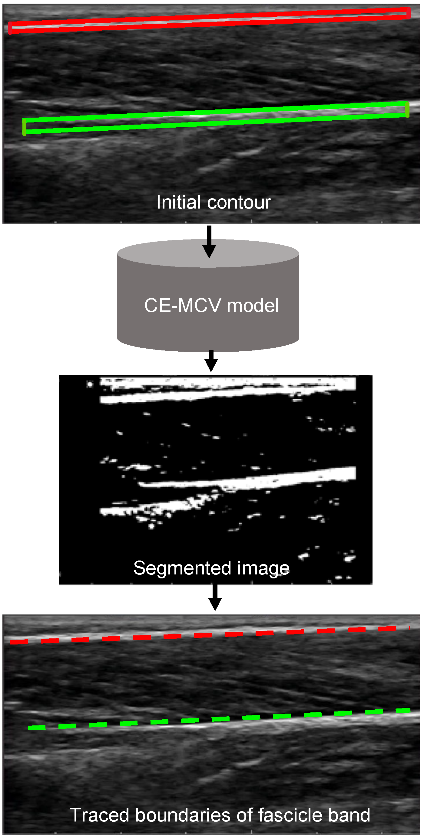
- Stage 1: Initialization
- Stage 2: Movement tracking of the deep and superficial aponeuroses
- Stage 3: Tracking of distortion in the fascicle band
- Stage 4: Calculation of FL and PA
2.1. Stage 1: Initialization
2.2. Stage 2: Tracking of Changes in Superficial and Deep Aponeuroses
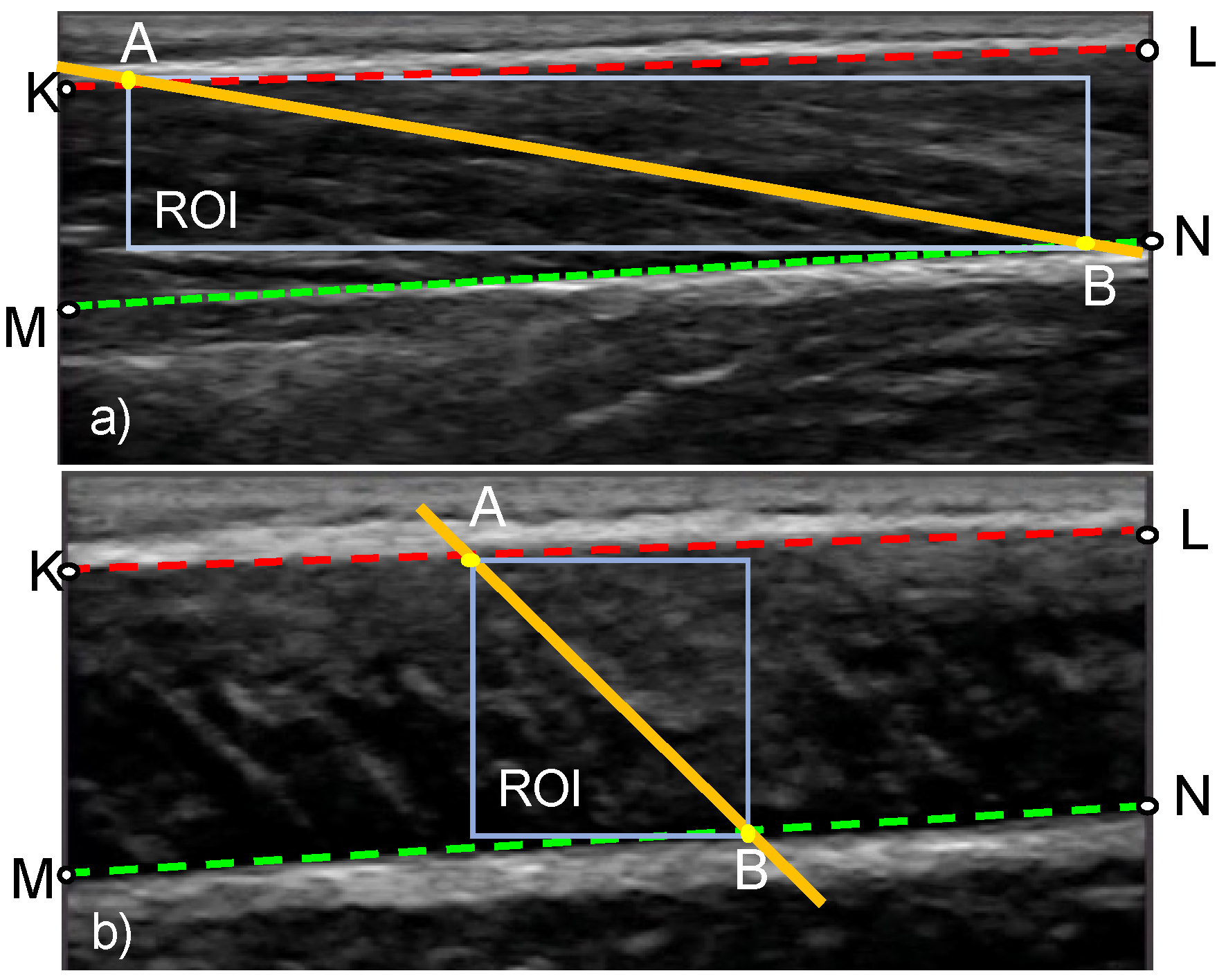
2.3. Stage 3: Tracking the Distortion in Fascicle Band
2.4. Stage 4: Calculation of PA and FL
3. Demonstration of the Proposed Approach
3.1. Comparison against Manual Measurements and Established Methods from Literature
3.2. Sensitivity to Initialization
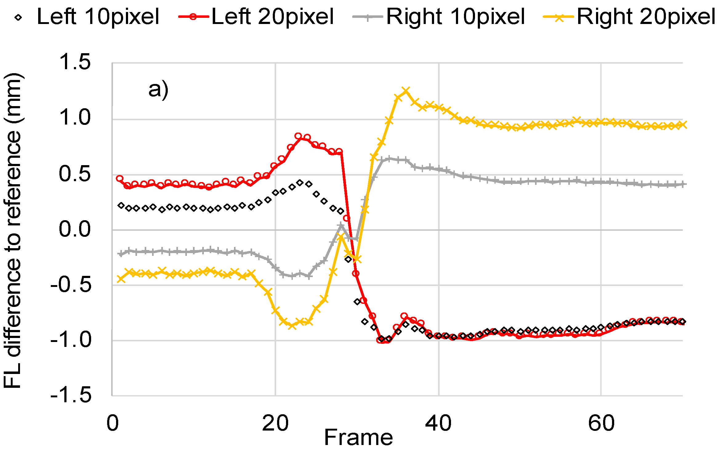
3.2.1. Parallel Shift of Fascicle Direction Line
3.2.2. Initial PA
4. Discussion
5. Conclusions
Author Contributions
Funding
Institutional Review Board Statement
Informed Consent Statement
Data Availability Statement
Acknowledgments
Conflicts of Interest
Appendix A
- Box sensitivity test for tracing of bottom and top boundaries of fascicle band:

References
- Maganaris, C.N.; Baltzopoulos, V.; Sargeant, A.J. In vivo measurements of the triceps surae complex architecture in man: Implications for muscle function. J. Physiol. 1998, 512, 603–614. [Google Scholar] [CrossRef] [PubMed]
- Stevens, D.E.; Smith, C.B.; Harwood, B.; Rice, C.L. In vivo measurement of fascicle length and pennation of the human anconeus muscle at several elbow joint angles. J. Anat. 2014, 225, 502–509. [Google Scholar] [CrossRef] [PubMed]
- Yuan, C.; Chen, Z.; Wang, M.; Zhang, J.; Sun, K.; Zhou, Y. Dynamic measurement of pennation angle of gastrocnemius muscles obtained from ultrasound images based on gradient Radon transform. Biomed. Signal Process. Control 2020, 55, 101604. [Google Scholar] [CrossRef]
- Zhou, G.-Q.; Chan, P.; Zheng, Y.-P. Automatic measurement of pennation angle and fascicle length of gastrocnemius muscles using real-time ultrasound imaging. Ultrasonics 2015, 57, 72–83. [Google Scholar] [CrossRef]
- Herbert, R.D.; Gandevia, S.C. Changes in pennation with joint angle and muscle torque: In vivo measurements in human brachialis muscle. J. Physiol. 1995, 484, 523–532. [Google Scholar] [CrossRef]
- Kawakami, Y.; Ichinose, Y.; Fukunaga, T. Architectural and functional features of human triceps surae muscles during contraction. J. Appl. Physiol. 1998, 85, 398–404. [Google Scholar] [CrossRef]
- Narici, M.V.; Binzoni, T.; Hiltbrand, E.; Fasel, J.; Terrier, F.; Cerretelli, P. In vivo human gastrocnemius architecture with changing joint angle at rest and during graded isometric contraction. J. Physiol. 1996, 496, 287–297. [Google Scholar] [CrossRef]
- Aggeloussis, N.; Giannakou, E.; Albracht, K.; Arampatzis, A. Reproducibility of fascicle length and pennation angle of gastrocnemius medialis in human gait in vivo. Gait Posture 2010, 31, 73–77. [Google Scholar] [CrossRef]
- Bohm, S.; Marzilger, R.; Mersmann, F.; Santuz, A.; Arampatzis, A. Operating length and velocity of human vastus lateralis muscle during walking and running. Sci. Rep. 2018, 8, 5066. [Google Scholar] [CrossRef]
- Damon, B.M.; Buck, A.K.; Ding, Z. Diffusion-tensor MRI-based skeletal muscle fiber tracking. Imaging Med. 2011, 3, 675–687. [Google Scholar] [CrossRef] [Green Version]
- Darby, J.; Li, B.; Costen, N.; Loram, I.; Hodson-Tole, E. Estimating Skeletal Muscle Fascicle Curvature From B-Mode Ultrasound Image Sequences. IEEE Trans. Biomed. Eng. 2013, 60, 1935–1945. [Google Scholar] [CrossRef] [PubMed]
- Darby, J.; Hodson-Tole, E.F.; Costen, N.; Loram, I.D. Automated regional analysis of B-mode ultrasound images of skeletal muscle movement. J. Appl. Physiol. 2012, 112, 313–327. [Google Scholar] [CrossRef] [PubMed]
- Marzilger, R.; Legerlotz, K.; Panteli, C.; Bohm, S.; Arampatzis, A. Reliability of a semi-automated algorithm for the vastus lateralis muscle architecture measurement based on ultrasound images. Eur. J. Appl. Physiol. 2018, 118, 291–301. [Google Scholar] [CrossRef]
- Monte, A.; Baltzopoulos, V.; Maganaris, C.N.; Zamparo, P. Gastrocnemius Medialis and Vastus Lateralis in vivo muscle-tendon behavior during running at increasing speeds. Scand. J. Med. Sci. Sports 2020, 30, 1163–1176. [Google Scholar] [CrossRef]
- Rekabizaheh, M.; Rezasoltani, A.; Lahouti, B.; Namavarian, N. Pennation Angle and Fascicle Length of Human Skeletal Muscles to Predict the Strength of an Individual Muscle Using Real-Time Ultrasonography: A Review of Literature. J. Clin. Physiother. Res. 2016, 1, 42–48. [Google Scholar] [CrossRef]
- Jeong, J.J.; Choi, H. An impedance measurement system for piezoelectric array element transducers. Measurement 2017, 97, 138–144. [Google Scholar] [CrossRef]
- Pohle-Fröhlich, R.; Dalitz, C.; Richter, C.; Stäudle, B.; Albracht, K. Estimation of Muscle Fascicle Orientation in Ultrasonic Images. arXiv 2019, arXiv:191204134. Available online: http://arxiv.org/abs/1912.04134 (accessed on 8 November 2021).
- Drazan, J.F.; Hullfish, T.J.; Baxter, J.R. An automatic fascicle tracking algorithm quantifying gastrocnemius architecture during maximal effort contractions. PeerJ 2019, 7, e7120. [Google Scholar] [CrossRef]
- Loram, I.D.; Maganaris, C.N.; Lakie, M. Use of ultrasound to make noninvasive in vivo measurement of continuous changes in human muscle contractile length. J. Appl. Physiol. 2006, 100, 1311–1323. [Google Scholar] [CrossRef]
- Cronin, N.J.; Finni, T.; Seynnes, O. Fully automated analysis of muscle architecture from B-mode ultrasound images with deep learning. arXiv 2020, arXiv:200904790. Available online: http://arxiv.org/abs/2009.04790 (accessed on 8 November 2021).
- Cunningham, R.; Harding, P.; Loram, I. Deep Residual Networks for Quantification of Muscle Fiber Orientation and Curvature from Ultrasound Images. In Medical Image Understanding and Analysis; Springer: Cham, Switzerland, 2017; pp. 63–73. [Google Scholar]
- Cronin, N.J.; Carty, C.P.; Barrett, R.S.; Lichtwark, G. Automatic tracking of medial gastrocnemius fascicle length during human locomotion. J. Appl. Physiol. 2011, 111, 1491–1496. [Google Scholar] [CrossRef] [PubMed]
- Rana, M.; Hamarneh, G.; Wakeling, J.M. Automated tracking of muscle fascicle orientation in B-mode ultrasound images. J. Biomech. 2009, 42, 2068–2073. [Google Scholar] [CrossRef] [PubMed]
- Cunningham, R.; Sánchez, M.; May, G.; Loram, I. Estimating Full Regional Skeletal Muscle Fibre Orientation from B-Mode Ultrasound Images Using Convolutional, Residual, and Deconvolutional Neural Networks. J. Imaging 2018, 4, 29. [Google Scholar] [CrossRef]
- Ramu, S.M.; Rajappa, M.; Krithivasan, K.; Jayakumar, J.; Chatzistergos, P.; Chockalingam, N. A method to improve the computational efficiency of the Chan-Vese model for the segmentation of ultrasound images. Biomed. Signal Process. Control 2021, 67, 102560. [Google Scholar] [CrossRef]
- Ki, N.; Delp, E. New Models for Real-Time Tracking Using Particle Filtering. In Visual Communications and Image Processing 2009; SPIE: San Jose, CA, USA, 2009; Volume 7257. [Google Scholar]
- Mei, X.; Ling, H. Robust visual tracking using ℓ1 minimization. In Proceedings of the 2009 IEEE 12th International Conference on Computer Vision, Kyoto, Japan, 29 September–2 October 2009; pp. 1436–1443. [Google Scholar] [CrossRef]
- Chen, F.; Wang, Q.; Wang, S.; Zhang, W.; Xu, W. Object tracking via appearance modeling and sparse representation. Image Vis. Comput. 2011, 29, 787–796. [Google Scholar] [CrossRef]
- Wang, L.; Yan, H.; Lv, K.; Pan, C. Visual Tracking Via Kernel Sparse Representation with Multikernel Fusion. IEEE Trans. Circuits Syst. Video Technol. 2014, 24, 1132–1141. [Google Scholar] [CrossRef]
- Liu, B.; Cheng, S.; Shi, Y. Particle Filter Optimization: A Brief Introduction. In Proceedings of the 7th International Conference in Swarm Intelligence, Bali, Indonesia, 25–30 June 2016; p. 104. [Google Scholar] [CrossRef]
- Mei, X.; Ling, H. Robust Visual Tracking and Vehicle Classification via Sparse Representation. IEEE Trans. Pattern Anal. Mach. Intell. 2011, 33, 2259–2272. [Google Scholar] [CrossRef]
- Gao, M.-L.; Li, L.-L.; Sun, X.-M.; Yin, L.-J.; Li, H.-T.; Luo, D.-S. Firefly algorithm (FA) based particle filter method for visual tracking. Optik 2015, 126, 1705–1711. [Google Scholar] [CrossRef]
- Bai, T.; Li, Y.F. Robust visual tracking with structured sparse representation appearance model. Pattern Recognit. 2012, 45, 2390–2404. [Google Scholar] [CrossRef]
- Mei, X.; Ling, H.; Wu, Y.; Blasch, E.; Bai, L. Minimum error bounded efficient ℓ1 tracker with occlusion detection. In Proceedings of the 2011 Conference on Computer Vision and Pattern Recognition (CVPR 2011), Colorado Springs, CO, USA, 20–25 June 2011; pp. 1257–1264. [Google Scholar] [CrossRef]
- Bao, C.; Wu, Y.; Ling, H.; Ji, H. Real time robust L1 tracker using accelerated proximal gradient approach. In Proceedings of the 2012 IEEE Conference on Computer Vision and Pattern Recognition, Providence, RI, USA, 16–21 June 2012; pp. 1830–1837. [Google Scholar] [CrossRef]
- Dahdouh, S.; Angelini, E.D.; Grange, G.; Bloch, I. Segmentation of embryonic and fetal 3D ultrasound images based on pixel intensity distributions and shape priors. Med. Image Anal. 2015, 24, 255–268. [Google Scholar] [CrossRef]
- Suri, J.S.; Farag, A.A. Deformable Models Theory and Biomaterial Applications, 1st ed.; Springer: New York, NY, USA, 2007. [Google Scholar] [CrossRef]
- Yuan, Y.; He, C. Adaptive active contours without edges. Math. Comput. Model. 2012, 55, 1705–1721. [Google Scholar] [CrossRef]
- Chen, Y.; Yue, X.; Da Xu, R.Y.; Fujita, H. Region scalable active contour model with global constraint. Knowl.-Based Syst. 2017, 120, 57–73. [Google Scholar] [CrossRef]
- Chan, T.F.; Vese, L.A. Active contours without edges. IEEE Trans. Image Process. 2001, 10, 266–277. [Google Scholar] [CrossRef] [PubMed]
- Alcantarilla, P.F.; Bartoli, A.; Davison, A.J. KAZE Features. In Proceedings of the 12th European Conference on Computer Vision (ECCV 2012), Florence, Italy, 7–13 October 2012; Springer: Berlin/Heidelberg, Germany, 2012; pp. 214–227. [Google Scholar]
- Choi, S.; Kim, T.; Yu, W. Performance evaluation of RANSAC family. In Proceedings of the British Machine Vision Conference, London, UK, 7–9 September 2009; Volume 24. [Google Scholar] [CrossRef]
- Kwah, L.K.; Pinto, R.Z.; Diong, J.; Herbert, R.D. Reliability and validity of ultrasound measurements of muscle fascicle length and pennation in humans: A systematic review. J. Appl. Physiol. 2013, 114, 761–769. [Google Scholar] [CrossRef] [Green Version]


| FL | PA | |||
|---|---|---|---|---|
| CoV | RMSE (mm) | CoV | RMSE (deg) | |
| Distortion-based approach | 4% | 2.4 ± 1.3 | 7% | 4.4 ± 1.4 |
| Feature tracking approach [18] | 4% | 2.7 ± 1.3 | 5% | 3.3 ± 1.7 |
| Feature detection approach [13] | 9% | 5.5 ± 2.6 | 16% | 8.8 ± 2.4 |
Publisher’s Note: MDPI stays neutral with regard to jurisdictional claims in published maps and institutional affiliations. |
© 2022 by the authors. Licensee MDPI, Basel, Switzerland. This article is an open access article distributed under the terms and conditions of the Creative Commons Attribution (CC BY) license (https://creativecommons.org/licenses/by/4.0/).
Share and Cite
Ramu, S.M.; Chatzistergos, P.; Chockalingam, N.; Arampatzis, A.; Maganaris, C. Automated Method for Tracking Human Muscle Architecture on Ultrasound Scans during Dynamic Tasks. Sensors 2022, 22, 6498. https://doi.org/10.3390/s22176498
Ramu SM, Chatzistergos P, Chockalingam N, Arampatzis A, Maganaris C. Automated Method for Tracking Human Muscle Architecture on Ultrasound Scans during Dynamic Tasks. Sensors. 2022; 22(17):6498. https://doi.org/10.3390/s22176498
Chicago/Turabian StyleRamu, Saru Meena, Panagiotis Chatzistergos, Nachiappan Chockalingam, Adamantios Arampatzis, and Constantinos Maganaris. 2022. "Automated Method for Tracking Human Muscle Architecture on Ultrasound Scans during Dynamic Tasks" Sensors 22, no. 17: 6498. https://doi.org/10.3390/s22176498