
Optimal Implementation Parameters of a Nonlinear Electrical Impedance Tomography Method Using the Complete Electrode Model

Department of Civil and Environmental Engineering, Hongik University, Seoul 04066, Korea
*
Author to whom correspondence should be addressed.
Sensors 2022, 22(17), 6667; https://doi.org/10.3390/s22176667
Submission received: 17 July 2022
/
Revised: 29 August 2022
/
Accepted: 31 August 2022
/
Published: 3 September 2022
(This article belongs to the Section Physical Sensors)
Abstract
:This study discusses a nonlinear electrical impedance tomography (EIT) technique under different analysis conditions to propose its optimal implementation parameters. The forward problem for calculating electric potential is defined by the complete electrode model. The inverse problem for reconstructing the target electrical conductivity profile is presented based on a partial-differential-equation-constrained optimization approach. The electrical conductivity profile is iteratively updated by solving the Karush–Kuhn–Tucker optimality conditions and using the conjugate gradient method with an inexact line search. Various analysis conditions such as regularization scheme, number of electrodes, current input patterns, and electrode arrangement were set differently, and the corresponding results were compared. It was found from this study that the proposed EIT method yielded appropriate inversion results with various parameter settings, and the optimal implementation parameters of the EIT method are presented. This study is expected to expand the utility and applicability of EIT for the non-destructive evaluation of structures.
1. Introduction
Electrical impedance tomography (EIT) is a non-destructive evaluation method through which the electrical properties of part of a structure are determined using measured data from surface electrodes. This method is highly applicable in medical imaging, industrial process monitoring, and geotechnical site characterization because of its ease of use in field experimentation, economic feasibility, and superior ability to penetrate the target. For example, the EIT method coupled with convolutional neural networks has been explored for reconstructing human organ boundaries [1], and EIT using an optimal control theory has been developed for pathological diagnoses such as cancer detection [2]. In industrial processes, EIT can be a useful tool to monitor the mixing process of chemical materials [3,4] and evaluate the dredging process’s condition in real-time by monitoring the material flowing through the dredging pipe [5,6]. Recent applications of EIT in civil engineering include the characterization of layered soils [7], crack detection in pipes buried in the ground [8], and ground contamination monitoring for remediation strategies [9].
EIT has many advantages; however, it requires improvements in its mathematical modeling, numerical analysis, and implementation techniques to increase the accuracy of solutions and to broaden its application scope to further extensive fields. Previous studies on EIT suggest that the quality of the inverse tomographic images obtained using measured electric potentials is sensitive to electrode arrangement and current input patterns [10,11,12,13,14,15,16]. Graham et al. [11] presented seven electrode placement configurations (planar, planar-offset, planar-opposite, zigzag, zigzag-offset, zigzag-opposite, square) in which the electrodes were arranged in two parallel planes of eight electrodes each, with electrodes equispaced around a medium. These configurations were applied to three-dimensional (3D) EIT, and the inversion results concerning the electrode arrangements were compared. Consequently, not one electrode placement configuration offered a good improvement over the others under ideal conditions. However, when noise and electrode placement errors are considered, the choice of electrode placement becomes important, and under that condition, planar electrode placement has the best overall performance. Schullcke et al. [12] evaluated the effect of different numbers of electrodes used for current injection and voltage measurements on the reconstructed two-dimensional shape of the lungs. The number of electrodes was varied systematically in steps of four, from to . According to the research results, the increased number of electrodes does not necessarily increase the image quality. The reconstructions made with 16 electrodes preserved the best quality.
Examples of current input patterns commonly used in EIT include the adjacent drive pattern [13], opposite or polar drive patterns [14], and trigonometric patterns [15]. The adjacent drive pattern is sensitive to conductivity contrasts near the boundary and insensitive to central contrasts. Furthermore, it is imperative to measurement errors and noise. The opposite or polar drive pattern is less sensitive to conductivity changes at the boundary in relation to the adjacent method, as the current travels with higher uniformity through the imaged body [16]. In the trigonometric pattern, the current is injected on all electrodes, and voltages are measured at all electrodes. This pattern results in more stable and accurate reconstruction than the adjacent current pattern. However, current drivers are required for each electrode to be injected, and the unknown contact impedance will affect the reconstruction [16,17,18].
Based on the previous developments, this study proposes several implementation parameters and analysis conditions for EIT, such as the number of electrodes, current input pattern, and electrode arrangement. The proposed parameters and analysis conditions are applied to the EIT procedure described in a recent study [19,20]. The EIT method is a nonlinear inversion based on a partial-differential-equation (PDE)-constrained optimization approach. By applying various implementation parameters, this study presents the optimal parameters of the EIT method that minimize relative -error or relative misfit. It also shows how much the quality of the reconstructed electrical conductivity profile using the optimal implementation parameters is improved in relation to the results using a conventional parameter set.
The remainder of this paper is organized as follows: In Section 2, the forward problem based on the complete electrode model (CEM) is presented. For verification, the forward solution was compared with that obtained using ANSYS Mechanical APDL [21]. In Section 3, the inverse medium problem is described, which derives the optimal solution using the Lagrangian functional and the first-order optimality conditions. The inversion process updates the electrical conductivity profile iteratively using a conjugate gradient method with an inexact line search. In Section 4, various numerical examples are described, wherein the regularization scheme, number of electrodes, current input pattern, and electrode arrangement are set differently. Optimal implementation parameters are suggested for the best reconstruction of a layered profile. Section 5 presents the conclusions of the study.
2. The Forward Problem
2.1. Mathematical Method
The CEM is a mathematical model for resolving the electrostatic forward problem for electric potential. It considers current loss that occurs when the current flows to a low-impedance material through an electrode and the voltage drop due to the contact impedance between the structural surface and electrode [22,23]. Therefore, the error between the calculated electric potential and experimentally obtained data is smaller than that computed using other models, such as a point electrode model. Figure 1 shows the configuration of a two-dimensional (2D) square domain with electrodes on its surface.
The CEM for calculating the electric potential due to the current input can be expressed as a boundary value problem, as follows:
where denotes structural domain, is the scalar-valued electric potential to be calculated, is electrical conductivity, is the outward unit normal to the boundary , is the electrode boundary, is the contact impedance of , is the injected current at , is the electric potential at to be calculated, and is the number of electrodes. Equation (1) is a Laplace equation for the electric potential . Equation (2) is a Robin-type boundary condition describing the electric potential at , and Equations (3) and (4) are Neumann boundary conditions for . To ensure the existence and uniqueness of the solution, the following continuity condition,
is added to the model. For setting the reference point of the electric potential,
must be satisfied. For the variational form of the boundary value problem, Equation (1) is multiplied by a test function , and then integrated over the domain using boundary conditions (2), (3), and (4). Meanwhile, Equation (2) is integrated over , multiplied by a test value , and then summed for all electrodes. Adding the two equations results in a variational form, expressed as follows [24]:
Introducing finite element approximations to the electric potential and the test function . results in a linear system of equations, where the electric potential at each node and the electrode potential can be calculated. The stiffness matrix and the right-hand-side vector of the linear system can be found in [19,20].
2.2. Setting for Numerical Analysis
The forward CEM solution is validated by comparing it to the solution obtained by ANSYS Mechanical APDL. Figure 2a shows the configuration of a homogeneous square domain with a side length of 10 m. The electrical conductivity of the domain is . A total of 10 electrodes are distributed equally on the left and right sides, as shown in the figure. Figure 2b shows a finite element model consisting of 1600 eight-node square elements with sides of 0.25 m. The length of one electrode is 0.25 m, equal to the size of the finite element. A current of 0.1 A is input into the electrodes placed on the left side of the domain, and it flows out through the electrodes placed on the right side. The contact impedance of the electrodes is .
2.3. Results of the Validation
Figure 3a,b show the distribution of the electric potential calculated by the CEM and ANSYS APDL, respectively, owing to the current input. In Figure 4, calculated electric potential values using the CEM and ANSYS APDL at nodes on , and are compared. It can be observed that the solutions obtained by the two different solvers are similar at all positions.
3. The Inverse Problem
3.1. PDE-Constrained Optimization
The inverse medium problem for reconstructing the electrical conductivity profile of a structure using measured electric potential data at surface electrodes can be presented as the following PDE-constrained optimization problem:
The objective functional comprises a misfit functional and a regularization term. The misfit functional is expressed as the sum of the squared differences of the calculated electric potential and the measured electric potential at electrode . This optimization problem is constrained by Equation (1), which is the governing equation of the CEM, and boundary conditions (2)–(4). To relieve the ill-posedness present in such an inverse problem, the regularization term for the electrical conductivity is included in the objective functional .
3.2. Regularization Schemes
In this study, Tikhonov (TN) [25] and total variation (TV) [26] regularization schemes are used to investigate the regularization effect. For TN regularization, the regularization term can be expressed by Equation (9):
For TV regularization, can be expressed by Equation (10):
where is a regularization factor that controls the penalty for the spatial variation of electrical conductivity . In Equation (10), a small parameter is included to make differentiable when . Generally, it is expected that TN regularization would be suitable for reconstructing a smooth target profile. On the other hand, TV regularization is expected to perform better when reconstructing a sharply varying target profile.
3.3. First-Order Optimality Conditions
The Lagrange multiplier method was used to convert the PDE-constrained optimization problem written in Equation (8) into an unconstrained optimization problem. The objective functional can be augmented using Equations (1) and (2) to construct the Lagrangian functional :
where and are Lagrange multipliers multiplied to the left-hand terms of the governing equation and boundary conditions, respectively. The electrical conductivity that minimizes the Lagrangian is the solution to the inverse problem. For the optimal solution to this problem, the first-order optimality conditions of the Lagrangian are enforced. In other words, the first variation of with respect to adjoint variables and , state variables and , and control variable is enforced to vanish. There results the state problem for and , the adjoint problem for and , and the control problem for , respectively. Solving the three problems simultaneously in the reduced space of the control variable yields the optimal solution of the material profile .
3.3.1. First Optimality Condition: State Problem
The state equation and the corresponding boundary conditions can be obtained from the stationarity requirement that the first variation of the Lagrangian with respect to adjoint variables and must be 0 ). The derived state problem is identical to the forward problem in Equations (1)–(4).
3.3.2. Second Optimality Condition: Adjoint Problem
The adjoint equation and the corresponding boundary conditions can be obtained from the stationarity requirement that the first variation of the Lagrangian with respect to state variables and must be 0 (). The derived adjoint problem can be described as follows [19,20]:
Equation (12) is the governing equation for the adjoint variable . It has a differential operator similar to (1), the state equation. Equations (13)–(15) are the boundary conditions of the adjoint problem. Equation (14) indicates the source of the adjoint problem, which depends on the misfit of the electric potential at electrodes. The adjoint problem can also be solved by the finite element method in a manner similar to the state problem [20].
3.3.3. Third Optimality Condition: Control Problem
The control equation and the corresponding boundary conditions can be obtained from the stationarity requirement that the first variation of the Lagrangian with respect to the control variable must be 0 (). The derived control problem can be described as follows [19,20]:
In deriving Equation (16), the TN regularization scheme was used. If the TV scheme were used instead, Equation (16) could be replaced by
where is the Hessian matrix of . It is different from the Hessian for the Gauss–Newton inversion, which consists of the second Fréchet derivatives of the Lagrangian [27,28,29]. The solution of the control problem can be calculated once the state and adjoint solutions , , and are obtained. The state, adjoint, and control problems derived from the first-order optimality conditions of the Lagrangian indicate the Karush–Kuhn–Tucker (KKT) conditions for this optimization problem.
3.4. Material Property Update
The first and second optimality conditions are satisfied by solving the state and adjoint problems, respectively. Because only the true profile of exactly satisfies the control problem, the material profile must be updated to satisfy the third optimality condition. The procedure of updating the control variable using the state and adjoint solutions is as follows:
- Assume the initial electrical conductivity profile of a structure to be investigated, then calculate the electric potential and due to the current input through the surface electrodes.
- Calculate the adjoint solutions and using the state solution .
- Using the state and adjoint solutions, calculate the gradient of the Lagrangian with respect to the control variable , as follows:In Equation (20), the TN regularization scheme was used. If the TV scheme were assumed, then the Lagrangian gradient for would be
- Update the electrical conductivity at each node using a line search method. Equations (17) and (18) are not precisely enforced in updating the electrical conductivity at boundaries since they are complicated to implement. Instead, one can enforce that the normal derivative of be zero along the boundary for computational simplicity.
3.5. Conjugate Gradient Method with an Inexact Line Search
The search direction for the optimal solution of the control variable is determined using the Fltcher–Reeves conjugate gradient method with an inexact line search. Let denote the discrete reduced gradient at the kth inversion iteration.
3.6. Regularization Factor Continuation Scheme
The choice of regularization factor in Equations (20) and (21) considerably affects the reconstruction of the electrical conductivity profile because it controls the amount of imposed penalty on high-frequency oscillations of the material properties. In this study, a regularization factor continuation scheme [30,31,32] was used to determine the optimal regularization factor at each inversion iteration. The reduced gradients in Equations (20) and (21) can be rewritten as
where denotes the gradient of the regularization functional and the gradient of the misfit functional. In the case of the TN regularization,
If the TV regularization scheme were used,
The first term of Equation (24), , penalizes spatial oscillations in the reconstructed profile, such that a higher results in a smoother reconstructed profile. A balance between these two terms can be imposed using
Therefore, can be calculated at each iteration as
where is a weight factor, which plays the role of regularization effect controller. results in the maximum regularization effect, and indicates no regularization.
4. Numerical Studies for Optimal EIT Parameters
Consider a square domain with a side length of , as shown in Figure 1, surrounded by electrodes with a contact impedance of . The initial value of the regularization factor is 1.0, and the weight factor for the regularization factor continuation scheme is set to 0.5. The parameter for TV regularization is assumed to be .
This study compares the inversion results according to the change in various implementation parameters using a response misfit and a relative -error. The response misfit , as part of the objective functional in Equation (8), can be written as
The relative -error of electrical conductivity, can be written as
where is the total area of the domain, is the target electrical conductivity, and is the reconstructed electrical conductivity.
4.1. Regularization Effect
For evaluating the regularization effect on the EIT, the TN and TV regularization schemes are explored in the inversion for a three-layer heterogeneous medium. Figure 5 shows the target electrical conductivity profile with three layers and an initial guess for inversion. The target values of the electrical conductivity are S/m for , S/m for , and S/m for . The values are typical of air-dried concrete materials in various conditions [33]. Examples of the profile heterogeneity in Figure 5 include fiber-reinforced composite sandwich plates and concrete specimens under curing. The initial guess for the inversion S/m. 40 electrodes are arranged on all sides of the square medium with equal spacing; thereafter, the current is injected into the electrodes attached on the top and left sides of the structure, and then flows out through the electrodes on the right and bottom sides. The magnitude of the current is uniform at 0.1 A.
Figure 6 shows the inversion results of the three-layer electrical conductivity profile at 3000 iterations using TN and TV regularization schemes. When the TV scheme was used, the target profile was reconstructed clearly and stably, especially at the interface of the layers. This shows that the TV scheme performs well in the EIT framework when reconstructing a sharply varying profile. Figure 7 shows the response misfit and the relative -error against iteration numbers. The misfit is reduced by 99.8% from its initial value for the TN scheme, and by 99.9% for the TV at 1500 iterations. Figure 8 shows the measured, initial, and calculated electric potentials in the inversion. After the inversion, the calculated potential values nearly coincide with the measured values, indicating the successful reconstruction of the target profile. Figure 9 shows the target and reconstructed conductivity profiles at , and in the domain. The results show that the recovered profile captures the variation of the target conductivity values in both directions.
As mentioned in Section 3.6, the regularization factor considerably affects the reconstruction of the electrical conductivity profile. Figure 10 shows the change in the regularization factor during the inversion using the regularization factor continuation scheme. The value of the weight factor was assumed to be 0.5, 0.3, 0.1, and 0.05. The higher the weight factor , the larger the value. It can also be seen that the value of fluctuates significantly in the latter part of the inversion as the inverted profile approaches the target.
For demonstrating the effectiveness of the regularization factor continuation scheme, the inversion tried fixed regularization factors in the same setting. Figure 11 and Figure 12 show the reconstructed three-layer electrical conductivity profiles using different fixed regularization factors. The layer interfaces are not properly recovered when is large, but the stratum is better reconstructed when the factor is small. Again, the TV scheme yielded sharper profile reconstruction than the TN. Compared to using fixed regularization factors, the continuation scheme determines the regularization factor adaptively at each inversion iteration, making it possible to skip multiple inversion attempts to find the optimal fixed regularization factor. Figure 13 shows the variation of the relative -error in Equation (32) to iteration numbers. In the case of the continuous regularization factor, the relative -error is similar to fixed regularization factor cases at the early inversion stage, but eventually becomes smaller as the inversion progresses.
4.2. Parametric Studies for Optimal EIT Result
In this study, three different analysis conditions were explored to derive optimal parameters for performing the EIT in heterogeneous media. The conditions considered are the number of electrodes, spatial current input pattern, and electrode arrangement. Figure 14 shows the target electrical conductivity profile with two layers and the initial guess for inversion. The target values of the electrical conductivity are S/m for and S/m for . The initial guess of the profile is homogeneous, with S/m. The TV regularization with the regularization factor continuation scheme is used in all parametric studies.
4.2.1. Number of Electrodes
The number of electrodes is expected to significantly affect the inversion result because it impacts the electric potential field and the amount of measured potential data. In this work, 8, 20, 40, and 80 electrodes are tested for inversion, as shown in Figure 15. An equal number of electrodes are placed on each side of the square medium. The current is supplied into the electrodes attached to the top and left sides of the medium, and then flows out from the electrodes on the right and bottom sides. The magnitude of the current is uniform at 0.1 A.
Figure 16 shows the reconstructed two-layer electrical conductivity profiles at 2000 inversion iterations using the presented number of electrodes. In the case of eight electrodes, the target profile is not reconstructed properly compared to other cases because the number of electrodes on the surface is significantly insufficient. In other cases, the target profile is reasonably reconstructed. Figure 17a shows the variation of response misfit to iteration numbers during the inversion. In the case of eight electrodes, the misfit changes extremely unstable, even for small iteration numbers. In other cases, decreases by a factor of to . Figure 17b exhibits the variation of the relative -error to iteration numbers. In the case of 20 electrodes, the error is smaller than 40 and 80 electrode cases after about 750 iterations. Thus, a higher number of electrodes does not necessarily increase the inversion quality. Figure 18 shows the measured, initial, and calculated electric potentials in the inversion using four different electrode numbers. After the inversion, the calculated potential values coincide with the measured values. Figure 19 shows the reconstructed electrical conductivity profiles at , and after the inversion using four different electrode numbers. Except for the case of eight electrodes, the calculated conductivity values capture the target sufficiently well in all locations. Figure 20 presents the inverted profiles using TN and TV regularization schemes in the case of eight surface electrodes. In comparison with the TV scheme, the inversion result has been improved in the case of TN regularization. Therefore, it is more appropriate to use TN regularization when the number of electrodes is small.
4.2.2. Current Input Pattern
Uniform and cosine input patterns are investigated as the current input pattern for inversion. The uniform pattern is the same as that used in Section 4.2.1. In the case of the cosine pattern, this study introduced four current input phases to the inversion. Equations (33) and (34) describe the uniform and cosine current input patterns, respectively.
In Equation (34), denotes the number of electrodes, and is a specific electrode number. In this numerical experiment, is 40, as shown in Figure 15c. Figure 21 shows the inverted two-layer electrical conductivity profiles at 2000 inversion iterations using the described current input patterns. Despite some differences in the results, especially at the layer interface, all current patterns successfully reconstructed the target profile. Figure 22 shows the response misfit and relative -error to iteration numbers in the inversion using the current input patterns. In all cases, the misfit is reduced by more than 99.9% from the initial misfit at 500 iterations. Figure 22b shows that the relative -error in the case of the uniform pattern is larger than that of the cosine patterns. The error is smallest when the phase . Figure 23 shows the measured, initial, and calculated electric potentials in the inversion using the current input patterns. Again, the calculated potential values are almost identical to the measured values. Figure 24 shows the reconstructed conductivity profiles at , and after the inversion using the current input patterns. All patterns reconstruct the target electrical conductivity profile fairly well.
4.2.3. Electrode Arrangement
Figure 25 shows two different types of electrode arrangements used for the EIT. The first arrangement type is to place electrodes on all sides of the medium, and the second is to position them only on two sides. The total number of electrodes is 40. The uniform and cosine ( current input patterns are used for this case.
Figure 26 shows the inversion results at 2000 iterations using the two electrode arrangements. The target profile has been reconstructed well for both current input patterns. However, the quality of reconstruction at the layer interface is better for the all-side arrangement. This happens when the electrodes are attached to only two sides of the structure, and the inner information of the top and bottom parts cannot be sufficiently captured by surface electrodes. Figure 27 shows the response misfit and the relative -error to iteration numbers during the inversion using the two electrode arrangements. For all cases, the misfit decreased by a factor of to . As shown in Figure 27b, the relative -error for the all-side arrangement is smaller than for the two-side arrangement. In addition, the error for the cosine current pattern is smaller than for the uniform pattern. Figure 28 shows the measured, initial, and calculated electric potentials in the inversion using the two electrode arrangements. The excellent agreement of the calculated and measured electric potential values demonstrates the feasibility of the inversion. Figure 29 presents the target and reconstructed electrical conductivity profiles at , and . Overall, the all-side arrangement results in better reconstruction of the target profile than the two-side arrangement.
4.3. Optimal Choice of Implementation Parameters
Figure 30 shows the variation of corresponding to the number of electrodes in the inversion using the all-side electrode arrangement. The values of were calculated after 2000 inversion iterations. As the number of electrodes increases, the relative -error tends to decrease. However, when the number of electrodes is 40 or more, there is a slight difference in the error. In addition, the error reduces when the cosine current input pattern is used, especially when or . A similar error trend can be observed in the case of the two-side electrode arrangement. Figure 31 presents the variation of corresponding to the number of electrodes in the inversion cases of different electrode arrangement and current input pattern. The relative -error is smaller in the case of the all-side electrode arrangement than in the two-side arrangement.
Table 2 and Table 3 show the relative -error and the relative misfit () for all cases of the number of electrodes, current input pattern, and electrode arrangement discussed so far. The misfit, , is the one immediately before the start of the misfit oscillation, and is the initial misfit. From the error values in the tables, one can choose the optimal implementation parameters of the described EIT. The first parameter set for which the value of is minimal is 80 electrodes, cosine current input pattern with , and the all-side electrode arrangement. The second parameter set for which the value of is minimal is the same as the first set except for the number of electrodes, which is 40. The minimum error values are shaded in the tables.
Figure 32 shows the reconstructed three-layer profiles using the optimal implementation parameters. The target and initial guess of the electrical conductivity profile are the same as those in Figure 5. The inverted profiles are obtained at 3000 iterations. The quality of profile reconstruction using the optimal parameter set is considerably better than the result shown in Figure 6, especially at the layer interface. Figure 33 shows the misfit and the relative -error against iteration numbers in the inversion using the optimal parameter sets. The relative -error decreased by 95.1% compared to the initial value when the first parameter set is used. It also decreased by 94.4% when using the second parameter set. The reduction rate of is slightly lower than in Figure 7b.
5. Conclusions
This study investigated optimal implementation parameters for a nonlinear EIT technique using the CEM. The EIT method is based on PDE-constrained optimization, which reconstructs the electrical conductivity profile by solving the KKT conditions iteratively. By applying various analysis conditions, the optimal set of parameters that minimize relative -error or relative misfit in the EIT has been derived. The quality of the reconstructed profile using the optimal implementation parameters is superior to the results using a conventional parameter set.
- The layered profile was reconstructed more clearly when using the TV regularization scheme than TN, especially at the interface of layers. The inversion result was improved when using the regularization factor continuation scheme rather than the fixed method.
- A higher number of electrodes did not necessarily improve the inversion results. In addition, the TN regularization scheme produced relevant results when the number of electrodes was small.
- The layered profiles were successfully reconstructed for all the presented current patterns. The relative -error was smaller when the cosine pattern was used, especially when the phase or .
- In the case of arranging electrodes on all sides of the square domain, the inversion result was improved compared to the case of arranging them only on two sides.
- The relative -error and the relative misfit are proper criteria for optimal implementation parameters. The relative -error was decreased by 95.1% from the initial value when using the first set of optimal parameters. It was also reduced by 94.4% when using the second set. The presented optimal parameter sets worked successfully in reconstructing layered electrical conductivity profiles.
This study is expected to expand the applicability of the nonlinear EIT method for the non-destructive evaluation of civil structures such as damage inspection, strength inspection of concrete under curing, fiber content inspection of fiber-reinforced concrete, etc.
Author Contributions
Conceptualization, J.W.K. and J.P.; methodology, J.W.K. and J.P.; software, J.P.; validation, J.W.K. and J.P.; formal analysis, J.W.K. and J.P.; investigation, J.W.K. and J.P.; resources, J.W.K. and E.C.; data curation, J.P.; writing—original draft preparation, J.P.; writing—review and editing, J.W.K.; visualization, J.P.; supervision, J.W.K. and E.C.; project administration, J.W.K. and E.C.; funding acquisition, J.W.K. and E.C. All authors have read and agreed to the published version of the manuscript.
Funding
This work was supported by the National Research Foundation of Korea under a grant from the Basic Science and Engineering Research Project (NRF-2017R1C1B200497515) and the grant from the Basic Laboratory Support Project (NRF-2020R1A4A101882611). It was also supported by Korea Hydro & Nuclear Power Co., Ltd. (No. 2019-TECH-01). The support received is greatly appreciated.
Institutional Review Board Statement
Not applicable.
Informed Consent Statement
Not applicable.
Data Availability Statement
The data that support the findings of this study are available from the corresponding author, Jun Won Kang, upon reasonable request.
Conflicts of Interest
The authors declare no conflict of interest.
Nomenclature
| Alphabetic symbols | |
| Area of square domain | |
| Search direction vector | |
| th electrode | |
| th electrode | |
| Force vector | |
| th inversion iteration | |
| Hessian matrix | |
| th electrode | |
| Current density | |
| Stiffness matrix | |
| Number of electrodes | |
| Number of nodes in finite element mesh | |
| Basis vector | |
| Regularization factor | |
| Vector consisting of electric potential at each electrode | |
| th electrode | |
| th electrode | |
| Solution vector | |
| Electric potential in domain | |
| Test value | |
| Test function | |
| Lagrange multiplier | |
| Lagrange multiplier | |
| th electrode | |
| Greek symbols | |
| Step length | |
| Initial step length | |
| Small parameter for TV regularization scheme | |
| th electrode | |
| Small parameter for Armijo condition | |
| Parameter for reducing step length | |
| Electrical conductivity | |
| Legendre basis function | |
| Structural domain | |
References
- Hamilton, S.J.; Hauptmann, A. Deep D-bar: Real-time electrical impedance tomography imaging with deep neural networks. IEEE Trans. Med. Imaging 2018, 37, 2367–2377. [Google Scholar] [CrossRef] [PubMed]
- Abdulla, U.G.; Bukshtynov, V.; Seif, S. Cancer detection through Electrical Impedance Tomography and optimal control theory: Theoretical and computational analysis. Math. Biosci. Eng. 2021, 18, 4834–4859. [Google Scholar] [CrossRef] [PubMed]
- Yenjaichon, W.; Grace, J.R.; Lim, C.J.; Bennington, C.P.J. In-line jet mixing of liquid–pulp–fibre suspensions: Effect of concentration and velocities. Chem. Eng. Sci. 2012, 75, 167–176. [Google Scholar] [CrossRef]
- Yenjaichon, W.; Grace, J.R.; Lim, C.J.; Bennington, C.P.J. Characterisation of gas mixing in water and pulp-suspension flow based on electrical resistance tomography. Chem. Eng. J. 2013, 214, 285–297. [Google Scholar] [CrossRef]
- Stevenson, R.; Harrison, S.T.L.; Miles, M.; Cilliers, J.J. Examination of swirling flow using electrical resistance tomography. Powder Technol. 2006, 162, 157–165. [Google Scholar] [CrossRef]
- Giguere, R.; Fradette, L.; Mignon, D.; Tanguy, P.A. Characterisation of slurry flow regime transitions by ERT. Chem. Eng. Res. Des. 2008, 86, 989–996. [Google Scholar] [CrossRef]
- Cheng, Q.; Tao, M.; Chen, X.; Binley, A. Evaluation of electrical resistivity tomography (ERT) for mapping the soil–rock interface in karstic environments. Environ. Earth Sci. 2019, 78, 439. [Google Scholar] [CrossRef]
- Jordana, J.; Gasulla, M.; Pallas-Areny., R. Electrical resistance tomography to detect leaks from buried pipes. Meas. Sci. Technol. 2001, 12, 1061–1068. [Google Scholar] [CrossRef]
- Ts, M.-E.; Lee, E.; Zhou, L.; Lee, K.H.; Seo, J.K. Remote real time monitoring for underground contamination in Mongolia using electrical impedance tomography. J. Nondestruct. Eval. 2006, 35, 8. [Google Scholar] [CrossRef]
- Kauppinen, P.; Hyttinen, J.; Malmivuo, J. Sensitivity distribution visualization of impedance tomography measurement strategies. Int. J. Bioelectromagn. 2016, 8, 63–71. [Google Scholar]
- Graham, B.H.; Adler, A. Electrode placement configuration for 3D EIT. Physiol. Meas. 2007, 28, S29–S44. [Google Scholar] [CrossRef] [PubMed]
- Schullcke, B.; Krueger-Ziolek, S.; Gong, B.; Moeller, K. Effect of the number of electrodes on the reconstructed lung shape in electrical impedance tomography. Curr. Dir. Biomed. Eng. 2006, 2, 499–502. [Google Scholar] [CrossRef]
- Brown, B.H.; Seagar, A.D. The Sheffield data collection system. Clin. Phys. Physiol. Meas. 1987, 8, 91–97. [Google Scholar] [CrossRef] [PubMed]
- Avis, N.J.; Barber, D.C. Image reconstruction using non-adjacent drive configurations. Physiol. Meas. 1994, 15, A153–A160. [Google Scholar] [CrossRef]
- Gisser, D.G.; Isaacson, D.; Newell, J.C. Current topics in impedance imaging. Clin. Phys. Physiol. Meas. 1987, 8, 39–46. [Google Scholar] [CrossRef]
- Harikumar, R.; Prabu, R.; Raghavan, S. Electrical impedance tomography (EIT) and its medical applications: A review. Int. J. Soft Comput. Eng. 2013, 3, 193–198. [Google Scholar]
- Dobson, D.C.; Santosa, F. Resolution and stability of an inverse problem in electrical impedance tomography: Dependence on the input current patterns. SIAM J. Appl. Math. 1994, 54, 1542–1560. [Google Scholar] [CrossRef]
- Kolehmainen, V.; Vauhkonen, M.; Karjalainen, P.A.; Kaipio, J.P. Assessment of errors in static electrical impedance tomography with adjacent and trigonometric current patterns. Physiol. Meas. 1997, 18, 289–303. [Google Scholar] [CrossRef]
- Jung, B.-G.; Kim, B.; Kang, J.W.; Hwang, J.-H. Electrode impedance tomography for material profile reconstruction of concrete structures. J. Comput. Struct. Eng. Inst. Korea 2019, 32, 249–256. [Google Scholar] [CrossRef]
- Jung, B.-G. Material Profile Reconstruction Using an Electrical Impedance Tomography Method Based on a Complete Electrode Model. Master’s Thesis, Hongik University, Seoul, Korea, 2019. [Google Scholar]
- ANSYS. Mechanical APDL Element References; ANSYS, Inc.: Canonsburg, PA, USA, 2016. [Google Scholar]
- Vauhkonen, P.J.; Vauhkonen, M.; Savolainen, T.; Kaipio, J.P. Three-dimensional electrical impedance tomography based on the complete electrode model. IEEE Trans. Biomed. Eng. 1999, 46, 1150–1160. [Google Scholar] [CrossRef]
- Cheng, K.; Isaacson, D.; Newell, J.C.; Gisser, D.G. Electrode models for electric current computed tomography. IEEE Trans. Biomed. Eng. 1989, 36, 918–924. [Google Scholar] [CrossRef] [PubMed]
- Somersalo, E.; Cheney, M.; Isaacson, D. Existence and uniqueness for electrode models for electric current computed tomography. SIAM J. Appl. Math. 1992, 52, 1023–1040. [Google Scholar] [CrossRef]
- Tikhonov, A.N. Solution of Incorrectly Formulated Problems and the Regularization Method. Sov. Math. Dokl. 1963, 4, 1035–1038. [Google Scholar]
- Rudin, L.I.; Osher, S.; Fatemi, E. Nonlinear total variation based noise removal algorithms. Phys. D Nonlinear Phenom. 1992, 60, 259–268. [Google Scholar] [CrossRef]
- Pakravan, A.; Kang, J.W. A Gauss-Newton Full-waveform Inversion for Material Profile Reconstruction in 1D PML-truncated Solid Media. KSCE J. Civ. Eng. 2014, 18, 1792–1804. [Google Scholar] [CrossRef]
- Pakravan, A.; Kang, J.W.; Newtson, C.M. A Gauss–Newton full-waveform inversion for material profile reconstruction in viscoelastic semi-infinite solid media. Inverse Probl. Sci. Eng. 2016, 24, 393–421. [Google Scholar] [CrossRef]
- Pakravan, A.; Kang, J.W.; Newtson, C.M. A Gauss–Newton full-waveform inversion in PML-truncated domains using scalar probing waves. J. Comput. Phys. 2017, 350, 824–846. [Google Scholar] [CrossRef]
- Kang, J.W.; Kallivokas, L.F. The inverse medium problem in 1D PML-truncated heterogeneous semi-infinite domains. Inverse Probl. Sci. Eng. 2010, 18, 759–786. [Google Scholar] [CrossRef]
- Kang, J.W.; Kallivokas, L.F. The inverse medium problem in heterogeneous PML-truncated domains using scalar probing waves. Comput. Methods Appl. Mech. Eng. 2011, 200, 265–283. [Google Scholar] [CrossRef]
- Joh, N.; Kang, J.W. Material profile reconstructing using plane electromagnetic waves in PML-truncated heterogeneous domains. Appl. Math. Modeling 2021, 96, 813–833. [Google Scholar] [CrossRef]
- Neville, A.M. Properties of Concrete; Longman: London, UK, 1995. [Google Scholar]
Figure 1.
Configuration of a two-dimensional square domain with surface electrodes.
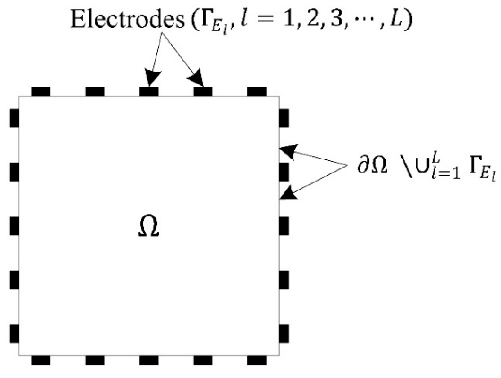
Figure 2.
(a) Configuration of a homogeneous square domain and (b) finite element mesh with eight-node quadrilateral elements.
Figure 2.
(a) Configuration of a homogeneous square domain and (b) finite element mesh with eight-node quadrilateral elements.
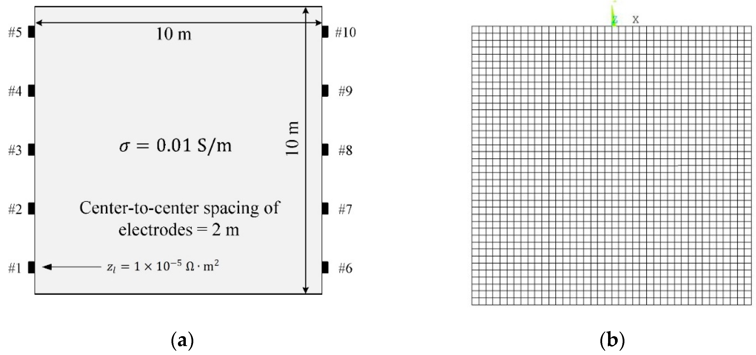
Figure 3.
Electric potential distribution calculated using CEM and ANSYS APDL. (a) CEM. (b) ANSYS APDL.
Figure 3.
Electric potential distribution calculated using CEM and ANSYS APDL. (a) CEM. (b) ANSYS APDL.

Figure 4.
Calculated electric potential values along particular lines in domain. (a) . (b) . (c) . (d) .
Figure 4.
Calculated electric potential values along particular lines in domain. (a) . (b) . (c) . (d) .

Figure 5.
Target electrical conductivity profile with three layers and the initial guess. (a) Target. (b) Initial guess.
Figure 5.
Target electrical conductivity profile with three layers and the initial guess. (a) Target. (b) Initial guess.
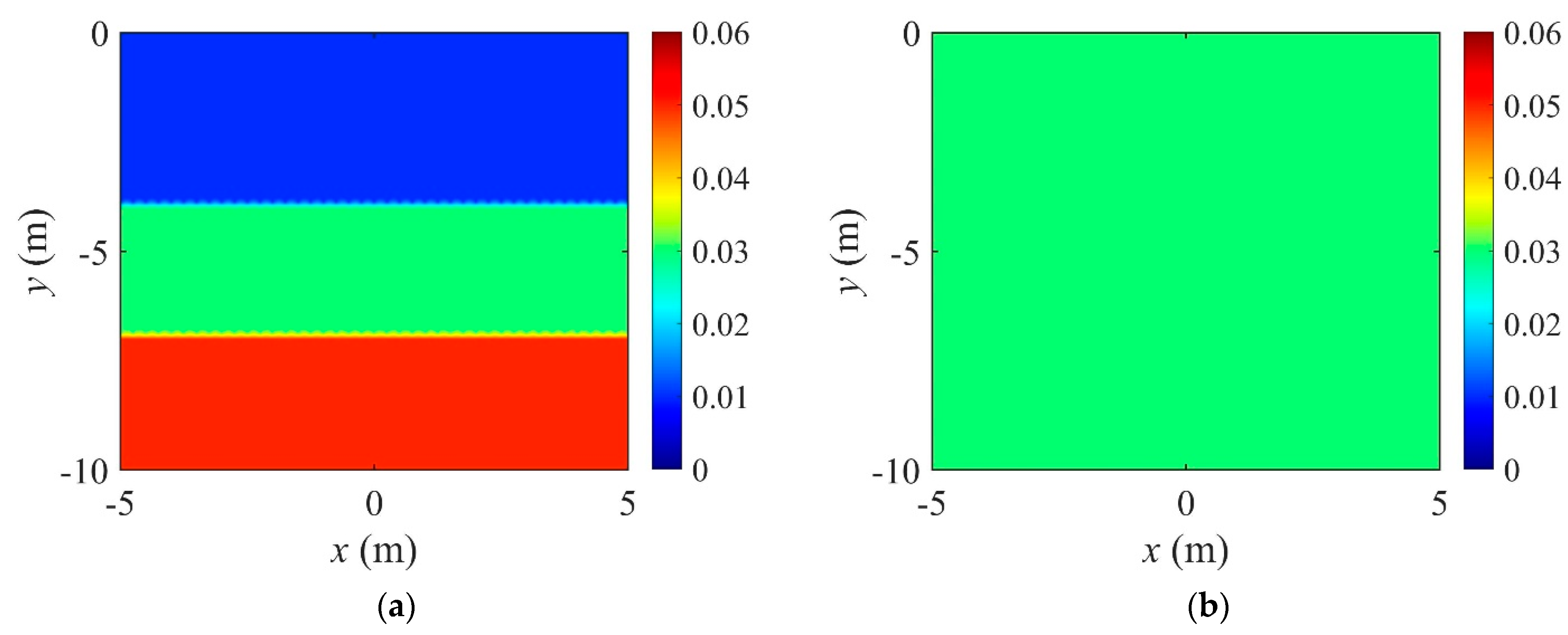
Figure 6.
Inversion results of a three-layer electrical conductivity profile using TN and TV regularization schemes. (a) TN. (b) TV.
Figure 6.
Inversion results of a three-layer electrical conductivity profile using TN and TV regularization schemes. (a) TN. (b) TV.
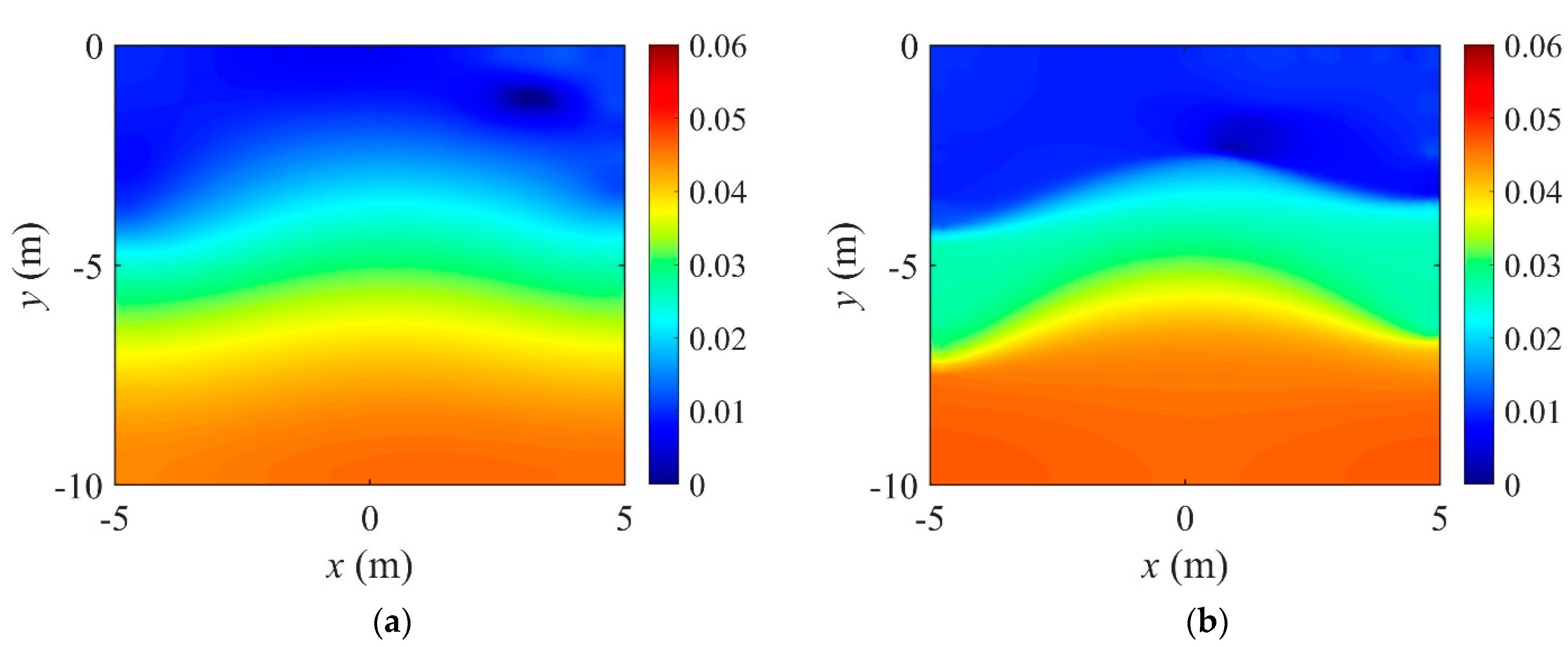
Figure 7.
Variation of response misfit and the relative -error during the inversion using TN and TV regularization schemes. (a) Misfit variation. (b) Relative -error.
Figure 7.
Variation of response misfit and the relative -error during the inversion using TN and TV regularization schemes. (a) Misfit variation. (b) Relative -error.
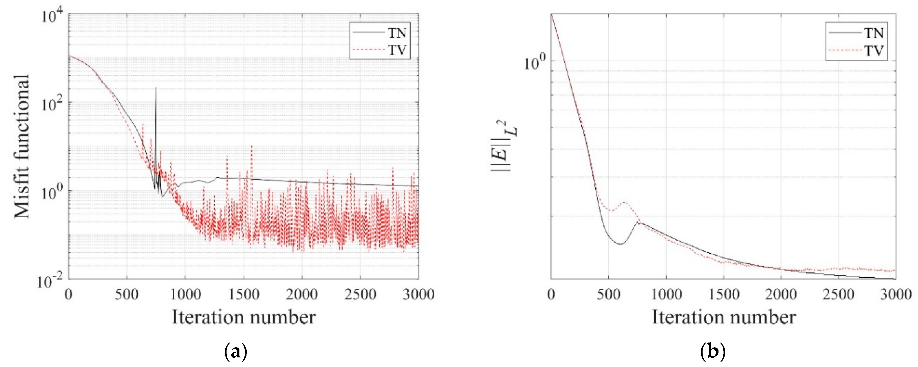
Figure 8.
Measured, initial, and calculated electric potentials in the inversion using TN and TV regularization schemes.
Figure 8.
Measured, initial, and calculated electric potentials in the inversion using TN and TV regularization schemes.

Figure 9.
Reconstructed conductivity profiles in the horizontal and vertical directions. (a) . (b) . (c) . (d) .
Figure 9.
Reconstructed conductivity profiles in the horizontal and vertical directions. (a) . (b) . (c) . (d) .

Figure 10.
Regularization factor variation during the inversion using the regularization factor continuation scheme. (a) TN. (b) TV.
Figure 10.
Regularization factor variation during the inversion using the regularization factor continuation scheme. (a) TN. (b) TV.

Figure 11.
Inversion for a three-layer profile using fixed regularization factors for TN regularization. (a) TN, . (b) TN, . (c) TN, .
Figure 11.
Inversion for a three-layer profile using fixed regularization factors for TN regularization. (a) TN, . (b) TN, . (c) TN, .
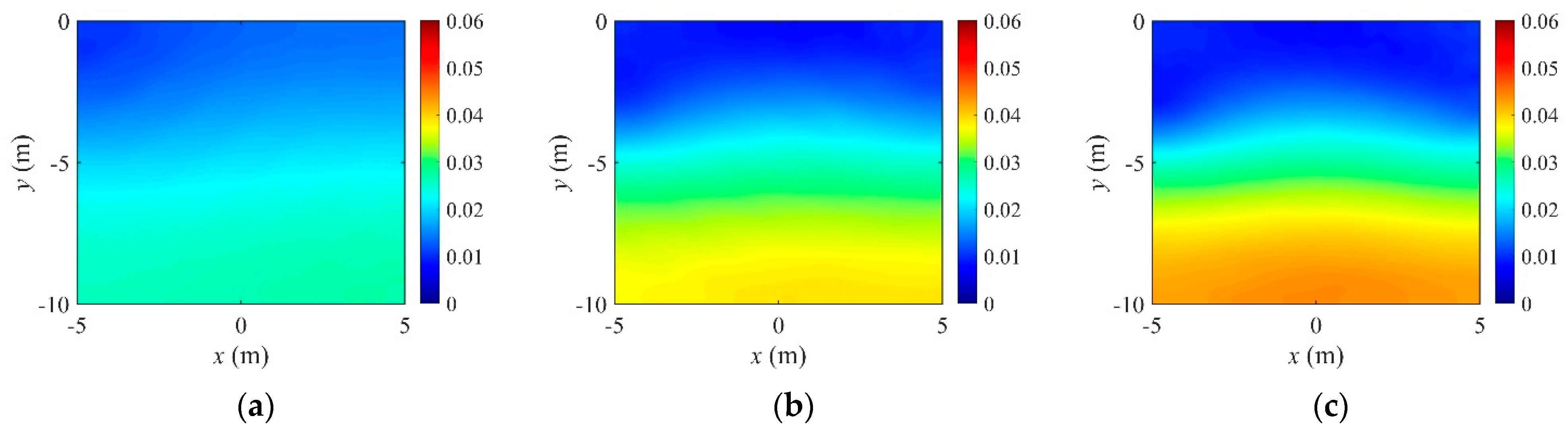
Figure 12.
Inversion for a three-layer profile using fixed regularization factors for TV regularization. (a) TV, . (b) TV, . (c) TV, .
Figure 12.
Inversion for a three-layer profile using fixed regularization factors for TV regularization. (a) TV, . (b) TV, . (c) TV, .

Figure 13.
Variation of to iteration numbers for fixed and continuous regularization factor schemes. (a) TN. (b) TV.
Figure 13.
Variation of to iteration numbers for fixed and continuous regularization factor schemes. (a) TN. (b) TV.
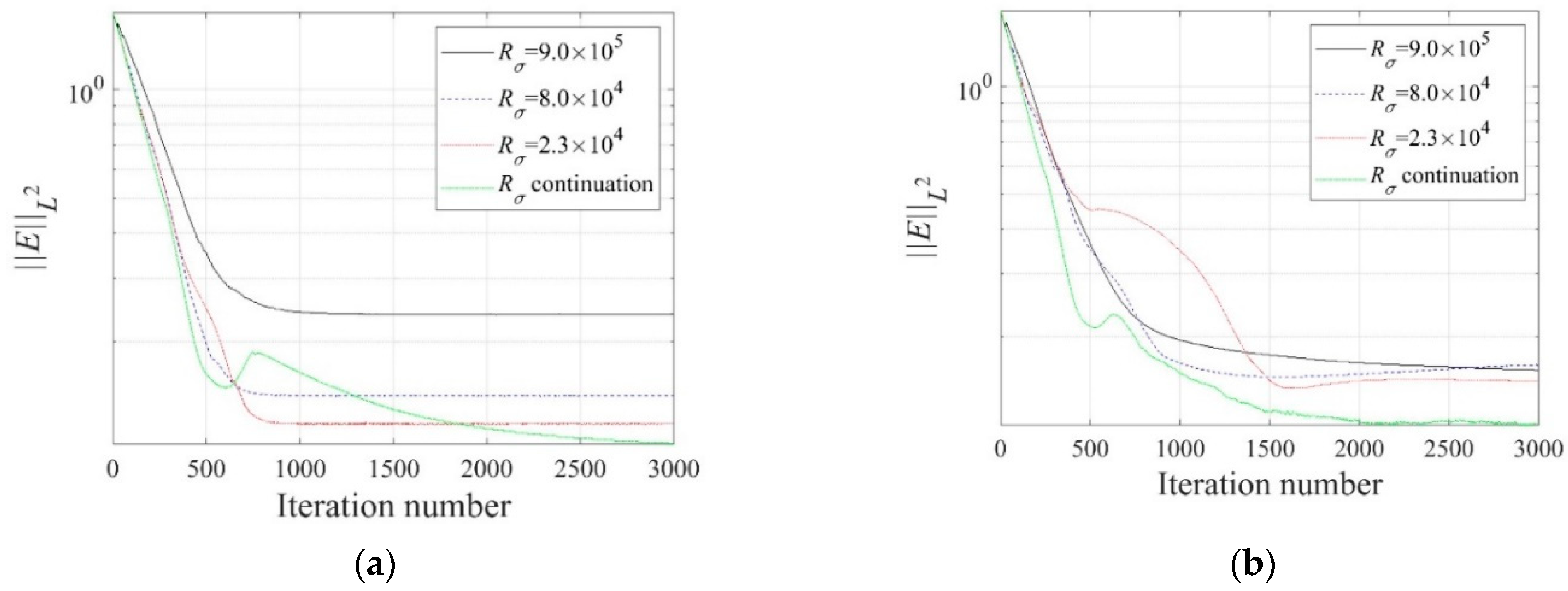
Figure 14.
Target electrical conductivity profile with two layers and the initial guess for inversion. (a) Target. (b) Initial guess.
Figure 14.
Target electrical conductivity profile with two layers and the initial guess for inversion. (a) Target. (b) Initial guess.
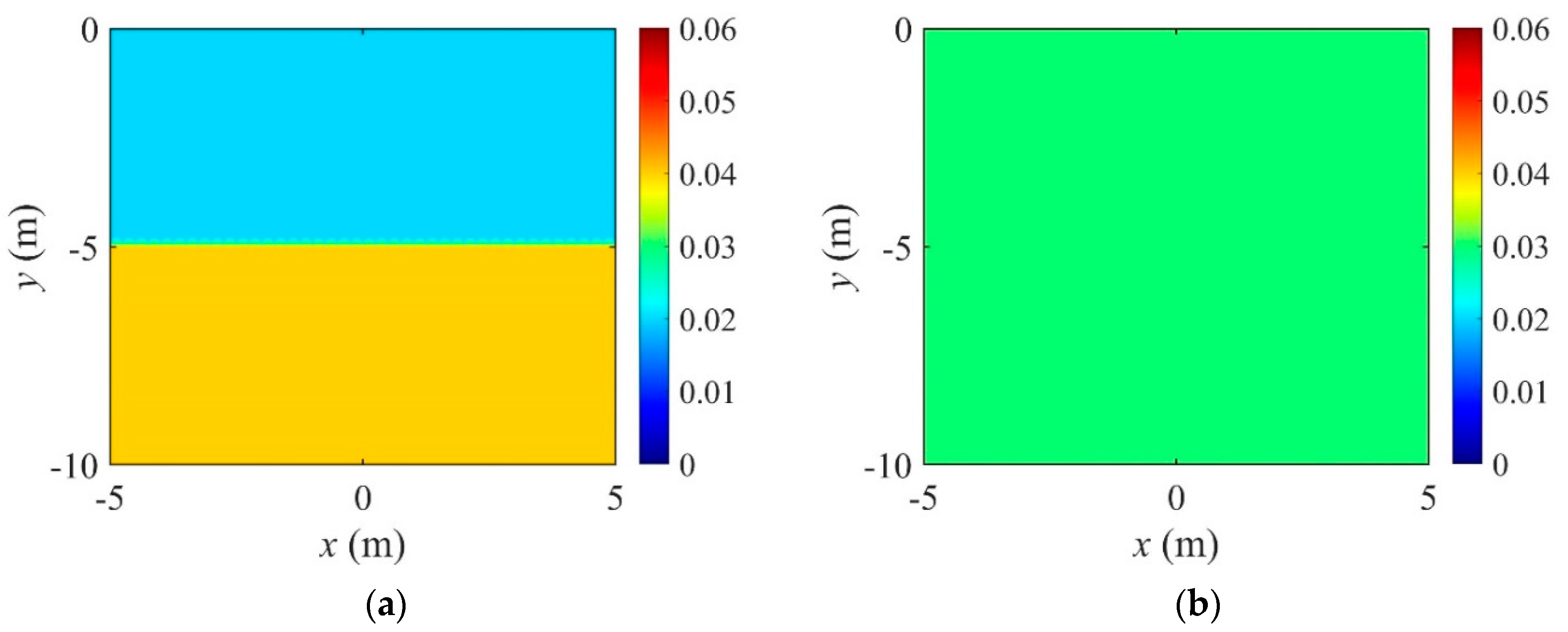
Figure 15.
Different number of electrodes for the EIT of a heterogeneous square medium: source electrode, top and left electrodes; receiver electrode, right and bottom electrodes. (a) 8 Electrodes. (b) 20 Electrodes. (c) 40 Electrodes. (d) 80 Electrodes.
Figure 15.
Different number of electrodes for the EIT of a heterogeneous square medium: source electrode, top and left electrodes; receiver electrode, right and bottom electrodes. (a) 8 Electrodes. (b) 20 Electrodes. (c) 40 Electrodes. (d) 80 Electrodes.

Figure 16.
Reconstructed two-layer electrical conductivity profiles using different number of electrodes. (a) 8 Electrodes. (b) 20 Electrodes. (c) 40 Electrodes. (d) 80 Electrodes.
Figure 16.
Reconstructed two-layer electrical conductivity profiles using different number of electrodes. (a) 8 Electrodes. (b) 20 Electrodes. (c) 40 Electrodes. (d) 80 Electrodes.

Figure 17.
Variation of response misfit and the relative -error to iteration numbers during the inversion using four different electrode numbers. (a) Misfit variation. (b) Relative -error.
Figure 17.
Variation of response misfit and the relative -error to iteration numbers during the inversion using four different electrode numbers. (a) Misfit variation. (b) Relative -error.
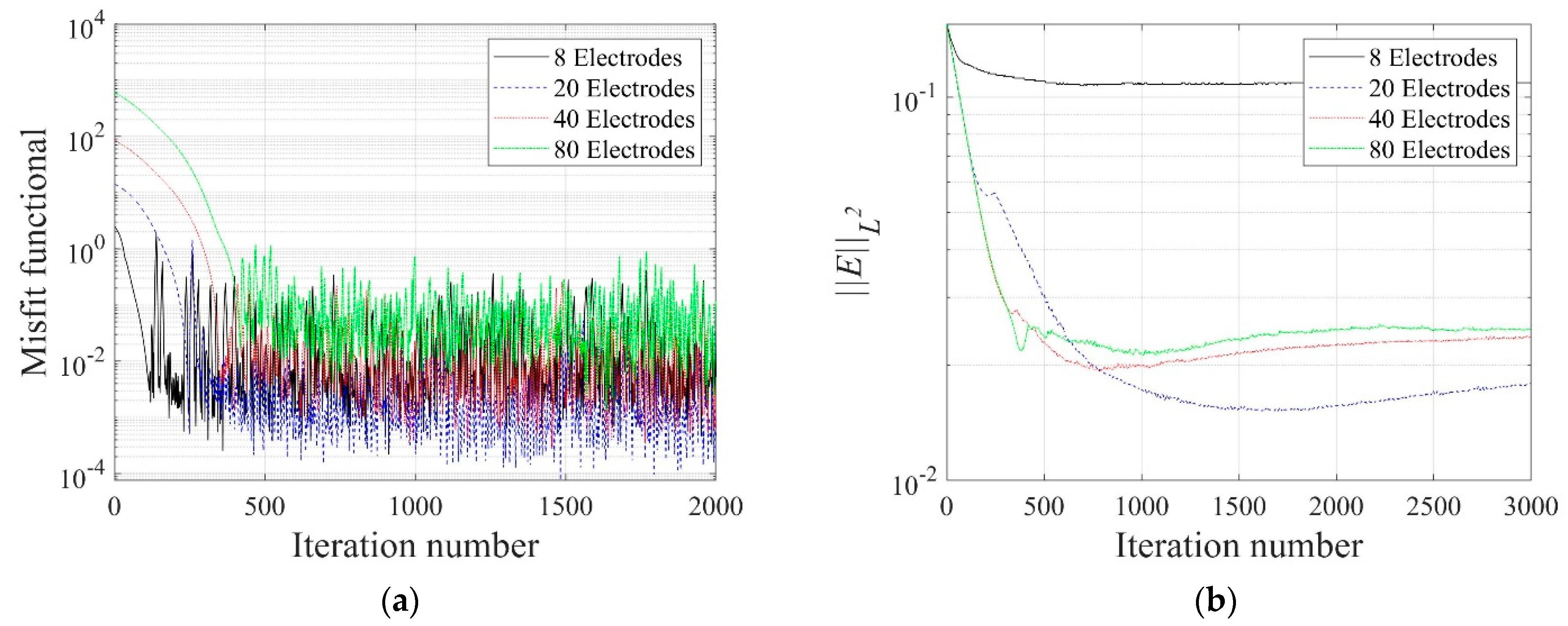
Figure 18.
Measured, initial, and calculated electric potentials in the inversion using four different electrode numbers. (a) 8 Electrodes. (b) 20 Electrodes. (c) 40 Electrodes. (d) 80 Electrodes.
Figure 18.
Measured, initial, and calculated electric potentials in the inversion using four different electrode numbers. (a) 8 Electrodes. (b) 20 Electrodes. (c) 40 Electrodes. (d) 80 Electrodes.

Figure 19.
Reconstructed electrical conductivity profiles at several locations of the domain after the inversion using four different electrode numbers. (a) . (b) . (c) . (d) .
Figure 19.
Reconstructed electrical conductivity profiles at several locations of the domain after the inversion using four different electrode numbers. (a) . (b) . (c) . (d) .

Figure 20.
Inverted two-layer conductivity profiles using TN and TV regularizations in the case of 8 electrodes. (a) TN. (b) TV.
Figure 20.
Inverted two-layer conductivity profiles using TN and TV regularizations in the case of 8 electrodes. (a) TN. (b) TV.

Figure 21.
Reconstructed two-layer electrical conductivity profiles using uniform and cosine current input patterns. (a) Uniform. (b) Cosine, . (c) Cosine, . (d) Cosine, . (e) Cosine, .
Figure 21.
Reconstructed two-layer electrical conductivity profiles using uniform and cosine current input patterns. (a) Uniform. (b) Cosine, . (c) Cosine, . (d) Cosine, . (e) Cosine, .

Figure 22.
Variation of response misfit and the relative -error to iteration numbers during the inversion using uniform and cosine current input patterns. (a) Misfit variation. (b) Relative -error.
Figure 22.
Variation of response misfit and the relative -error to iteration numbers during the inversion using uniform and cosine current input patterns. (a) Misfit variation. (b) Relative -error.
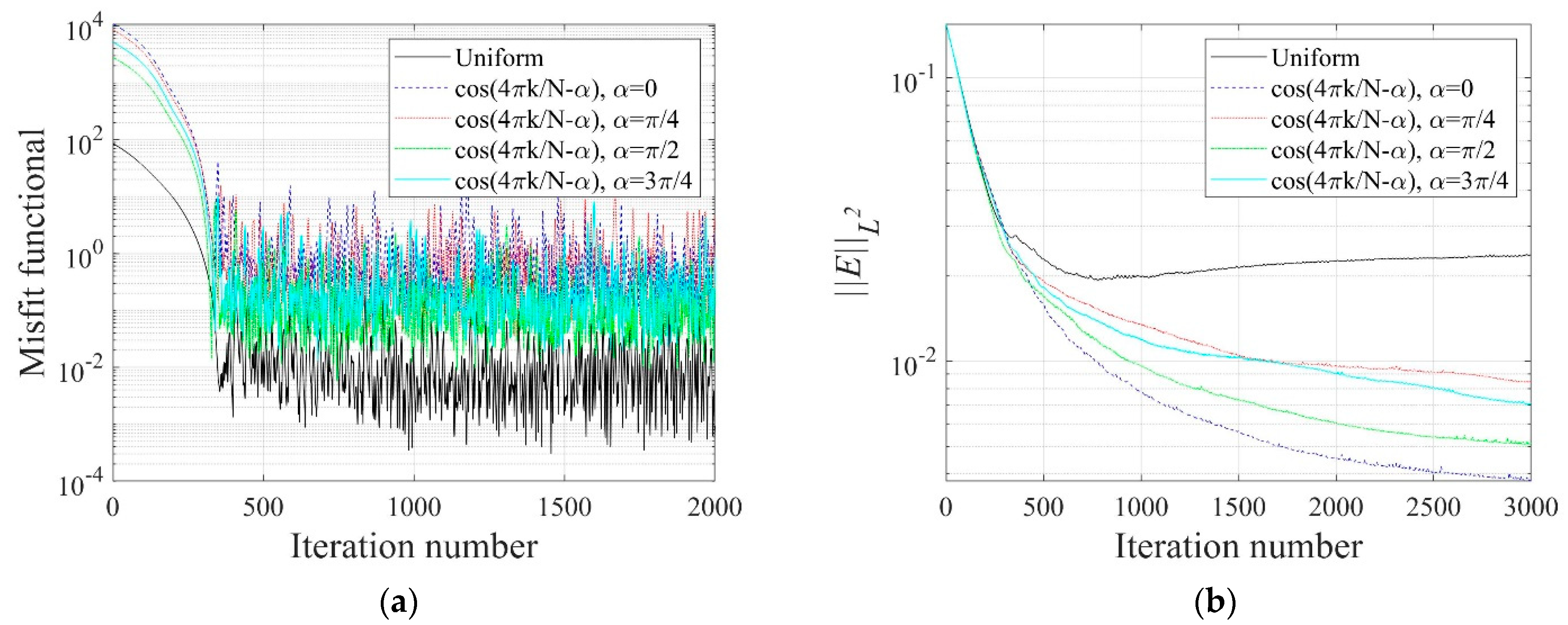
Figure 23.
Measured, initial, and calculated electric potentials in the inversion using uniform and cosine current input patterns. (a) Uniform. (b) Cosine, . (c) Cosine, . (d) Cosine, . (e) Cosine, .
Figure 23.
Measured, initial, and calculated electric potentials in the inversion using uniform and cosine current input patterns. (a) Uniform. (b) Cosine, . (c) Cosine, . (d) Cosine, . (e) Cosine, .

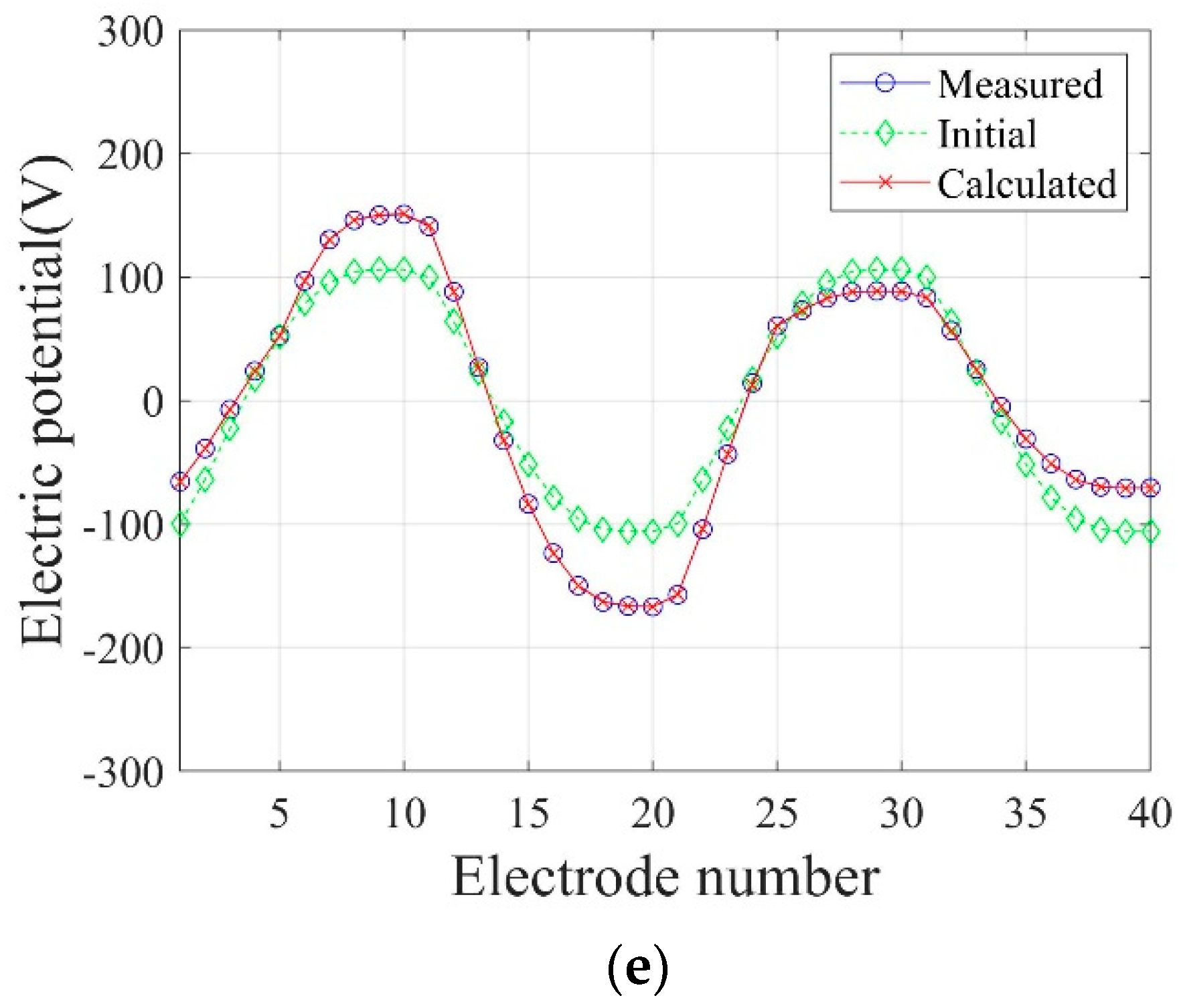
Figure 24.
Reconstructed electrical conductivity profiles at several locations of the domain in the inversion using uniform and cosine current input patterns. (a) . (b) . (c) . (d) .
Figure 24.
Reconstructed electrical conductivity profiles at several locations of the domain in the inversion using uniform and cosine current input patterns. (a) . (b) . (c) . (d) .

Figure 25.
Configuration of two different types of electrode arrangement; For the uniform current input pattern, the source electrode is #1 to #20, and receiver electrode is #21 to #40. For the cosine input pattern with , source and receiver electrodes are determined per Equation (34). (a) All-side. (b) Two-side.

Figure 26.
Reconstructed two-layer electrical conductivity profiles using two electrode arrangements. (a) All-side, uniform. (b) All-side, cosine, . (c) Two-side, uniform. (d) Two-side, cosine, .
Figure 26.
Reconstructed two-layer electrical conductivity profiles using two electrode arrangements. (a) All-side, uniform. (b) All-side, cosine, . (c) Two-side, uniform. (d) Two-side, cosine, .
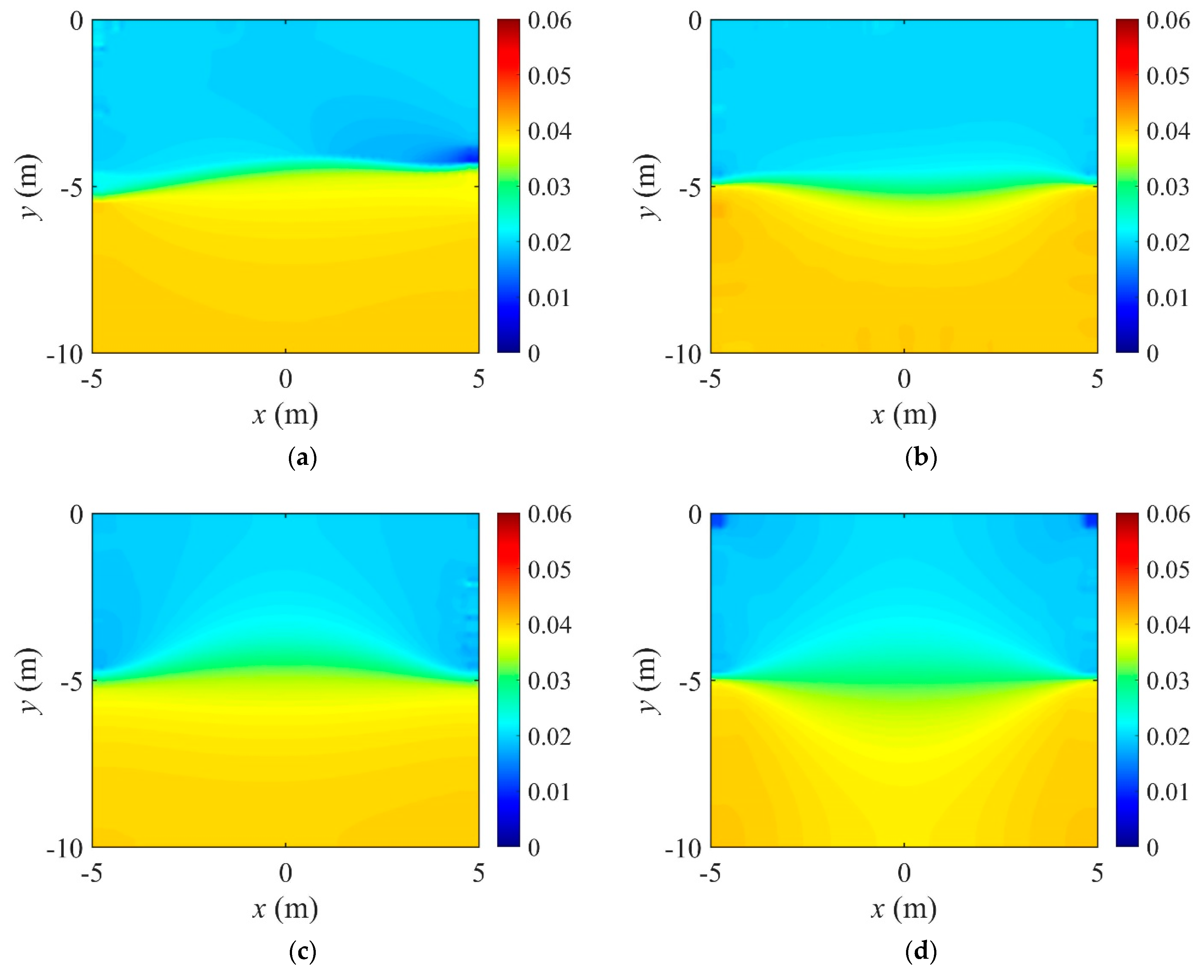
Figure 27.
Variation of response misfit and the relative -error to iteration numbers during the inversion using two electrode arrangements. (a) Misfit variation. (b) Relative -error.
Figure 27.
Variation of response misfit and the relative -error to iteration numbers during the inversion using two electrode arrangements. (a) Misfit variation. (b) Relative -error.

Figure 28.
Measured, initial, and calculated electric potentials in the inversion using two electrode arrangements. (a) All-side, uniform. (b) All-side, cosine, . (c) Two-side, uniform. (d) Two-side, cosine, .
Figure 28.
Measured, initial, and calculated electric potentials in the inversion using two electrode arrangements. (a) All-side, uniform. (b) All-side, cosine, . (c) Two-side, uniform. (d) Two-side, cosine, .
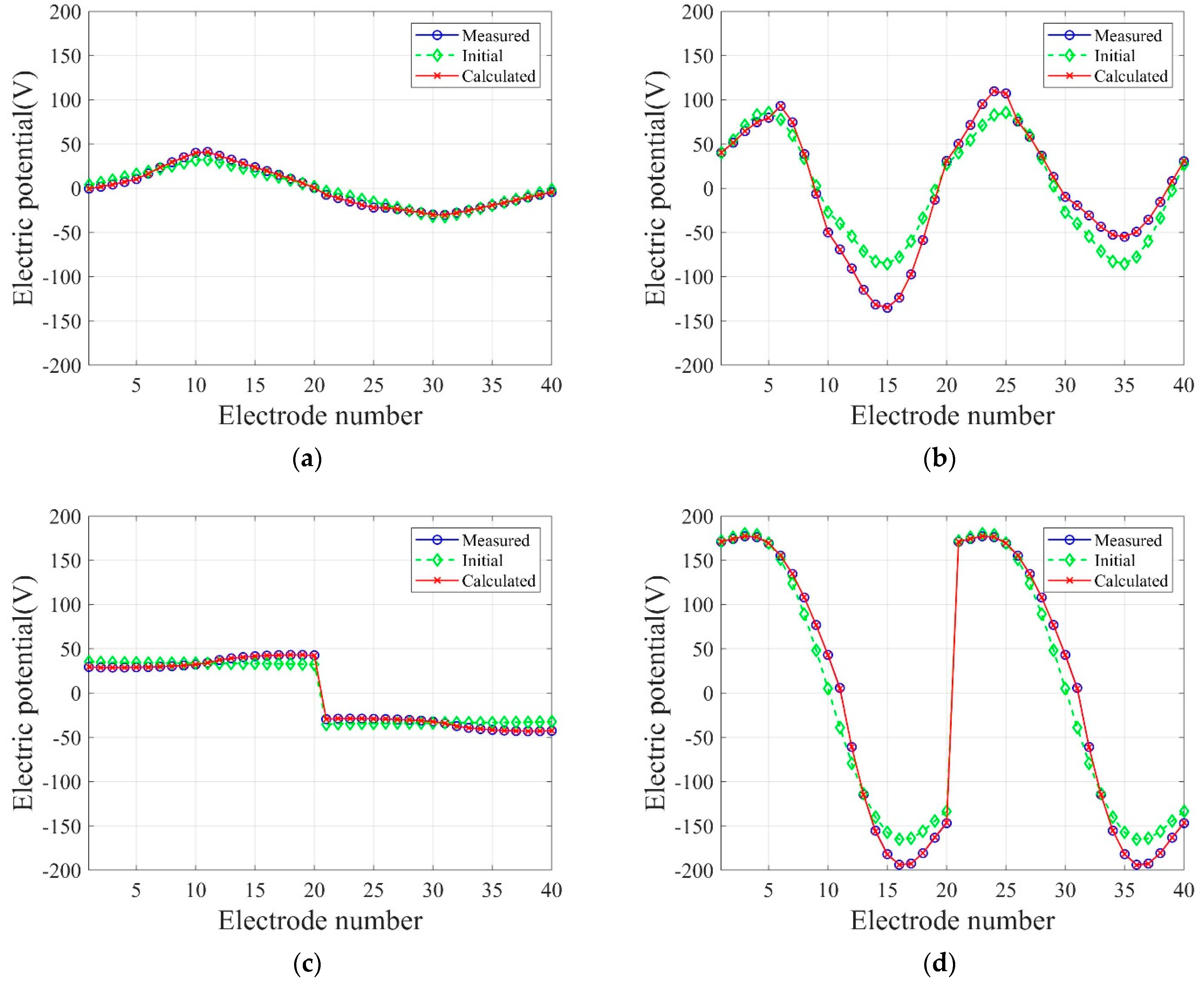
Figure 29.
Reconstructed electrical conductivity profiles at several locations of the domain in the inversion using two electrode arrangements. (a) . (b) . (c) . (d) .
Figure 29.
Reconstructed electrical conductivity profiles at several locations of the domain in the inversion using two electrode arrangements. (a) . (b) . (c) . (d) .
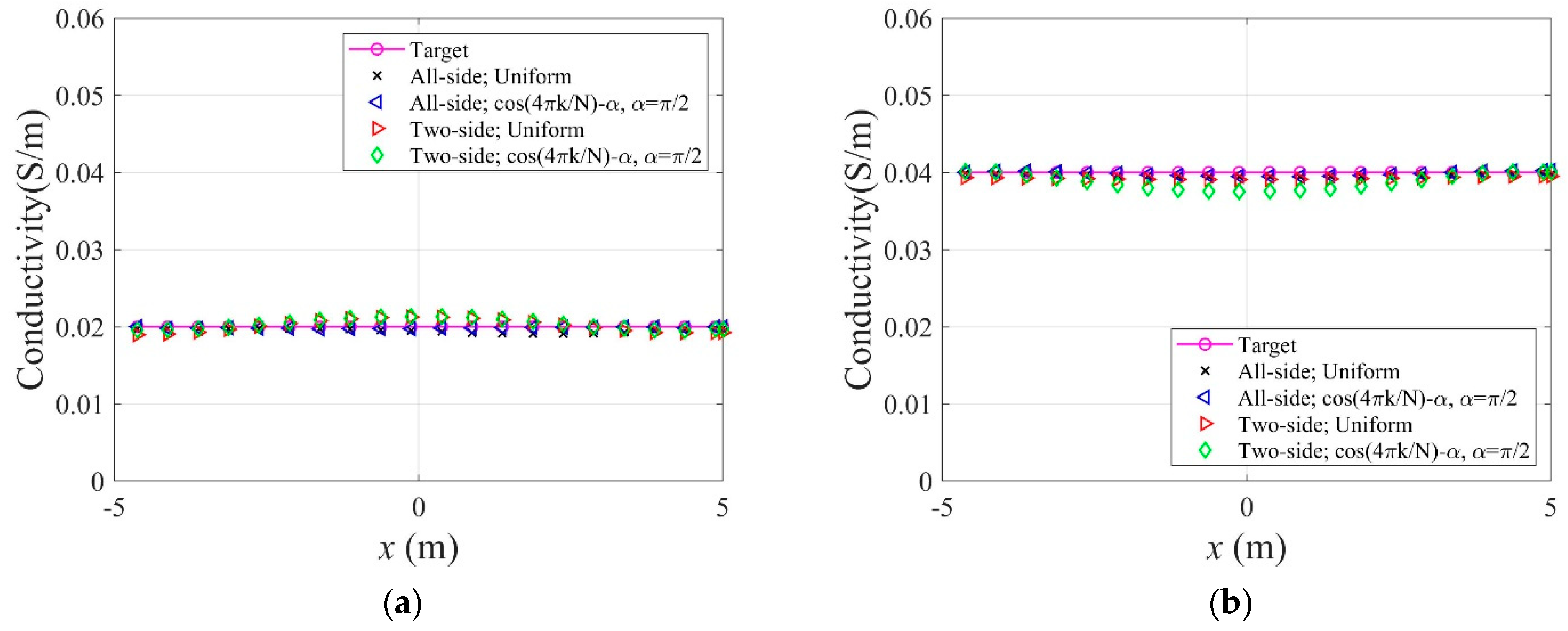
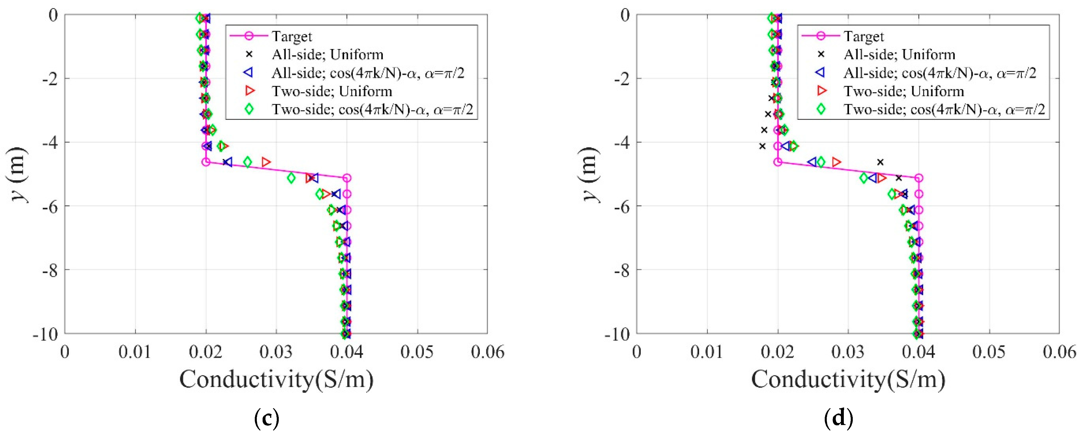
Figure 30.
Variation of corresponding to the number of electrodes in the inversion using the all-side electrode arrangement; the values were calculated at 2000 inversion iterations.
Figure 30.
Variation of corresponding to the number of electrodes in the inversion using the all-side electrode arrangement; the values were calculated at 2000 inversion iterations.

Figure 31.
Variation of corresponding to the number of electrodes in the inversion cases of different electrode arrangement and current input pattern; the values were calculated at 2000 inversion iterations.
Figure 31.
Variation of corresponding to the number of electrodes in the inversion cases of different electrode arrangement and current input pattern; the values were calculated at 2000 inversion iterations.

Figure 32.
Reconstructed three-layer electrical conductivity profiles using the optimal implementation parameters. (a) First parameter set. (b) Second parameter set.
Figure 32.
Reconstructed three-layer electrical conductivity profiles using the optimal implementation parameters. (a) First parameter set. (b) Second parameter set.

Figure 33.
Response misfit and relative -error against iteration numbers in the inversion using the optimal implementation parameters. (a) Misfit variation. (b) Relative -error.
Figure 33.
Response misfit and relative -error against iteration numbers in the inversion using the optimal implementation parameters. (a) Misfit variation. (b) Relative -error.

Table 1.
Backtracking algorithm to determine the step length .
| Choose , , set repeat until Terminate with |
Table 2.
Relative -error, , for all the inversion cases of this study.
| Current Input Pattern | Electrode Arrangement | |||||||
|---|---|---|---|---|---|---|---|---|
| All-Side Arrangement | Two-Side Arrangement | |||||||
| Number of Electrodes | Number of Electrodes | |||||||
| 8 | 20 | 40 | 80 | 8 | 20 | 40 | 80 | |
| Uniform | ||||||||
| Cosine, | ||||||||
| Cosine, | ||||||||
| Cosine, | ||||||||
| Cosine, | ||||||||
Table 3.
Relative misfit, , for all the inversion cases of this study.
| Current Input Pattern | Electrode Arrangement | |||||||
|---|---|---|---|---|---|---|---|---|
| All-Side Arrangement | Two-Side Arrangement | |||||||
| Number of Electrodes | Number of Electrodes | |||||||
| 8 | 20 | 40 | 80 | 8 | 20 | 40 | 80 | |
| Uniform | ||||||||
| Cosine, | ||||||||
| Cosine, | ||||||||
| Cosine, | ||||||||
| Cosine, | ||||||||
Publisher’s Note: MDPI stays neutral with regard to jurisdictional claims in published maps and institutional affiliations. |
© 2022 by the authors. Licensee MDPI, Basel, Switzerland. This article is an open access article distributed under the terms and conditions of the Creative Commons Attribution (CC BY) license (https://creativecommons.org/licenses/by/4.0/).
Share and Cite
MDPI and ACS Style
Park, J.; Kang, J.W.; Choi, E. Optimal Implementation Parameters of a Nonlinear Electrical Impedance Tomography Method Using the Complete Electrode Model. Sensors 2022, 22, 6667. https://doi.org/10.3390/s22176667
AMA Style
Park J, Kang JW, Choi E. Optimal Implementation Parameters of a Nonlinear Electrical Impedance Tomography Method Using the Complete Electrode Model. Sensors. 2022; 22(17):6667. https://doi.org/10.3390/s22176667
Chicago/Turabian StylePark, Jeongwoo, Jun Won Kang, and Eunsoo Choi. 2022. "Optimal Implementation Parameters of a Nonlinear Electrical Impedance Tomography Method Using the Complete Electrode Model" Sensors 22, no. 17: 6667. https://doi.org/10.3390/s22176667
Note that from the first issue of 2016, this journal uses article numbers instead of page numbers. See further details here.