
A Novel Approach for UAV Image Crack Detection


Abstract
:1. Introduction
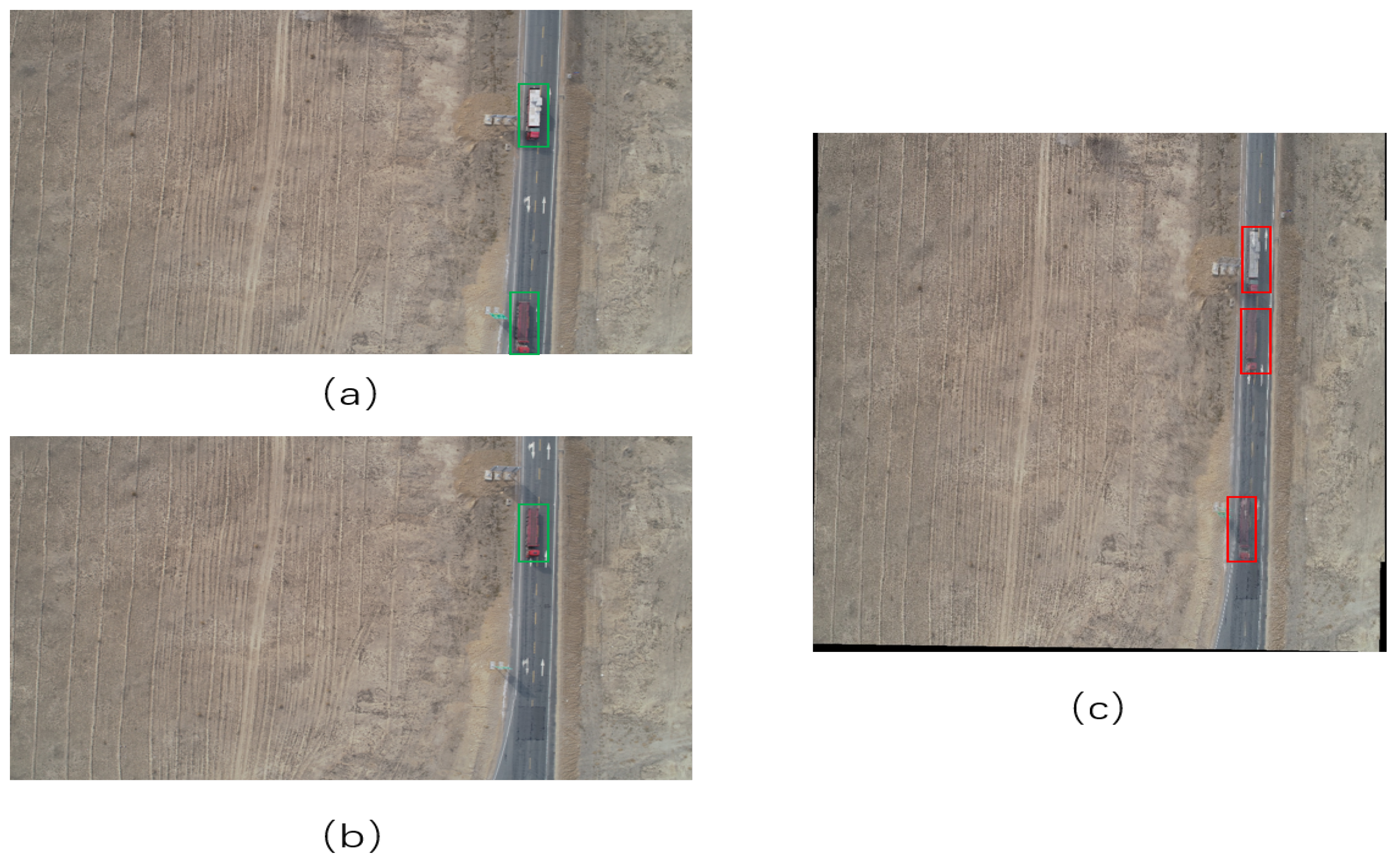
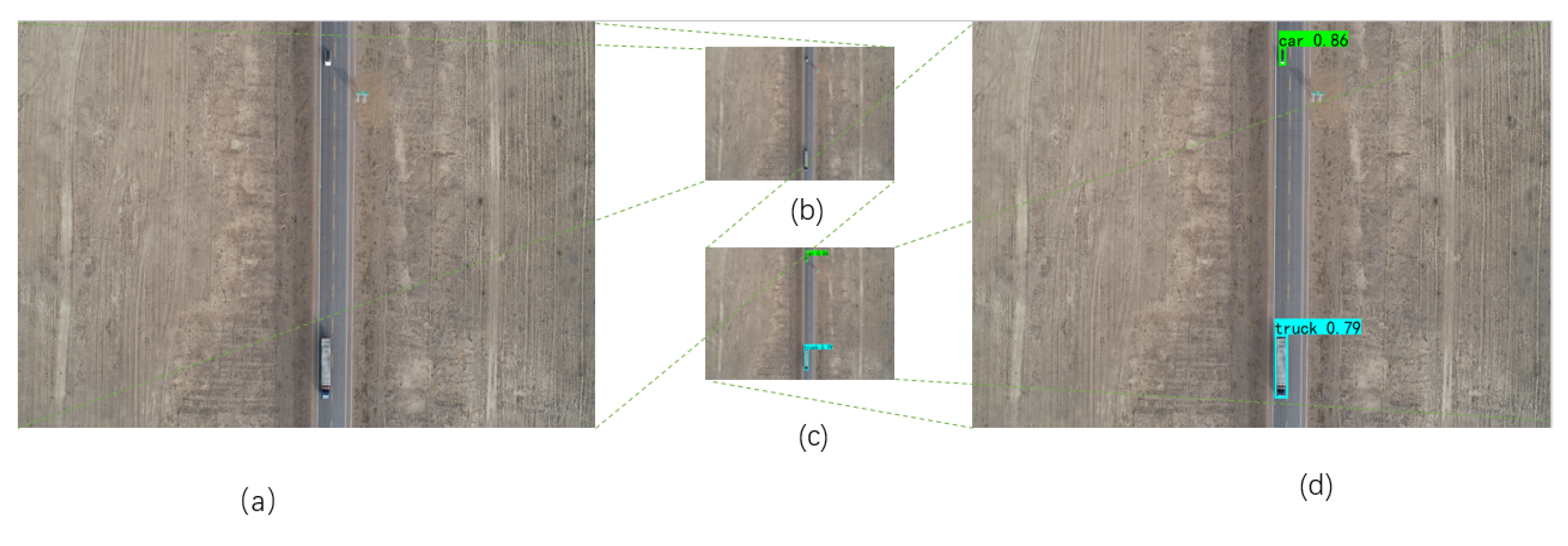
- The problem of multiple images with duplicate regions and the problem of images with occlusion are proposed for the first time, and an innovative way of combining target detection and image stitching is used to deal with these two problems.
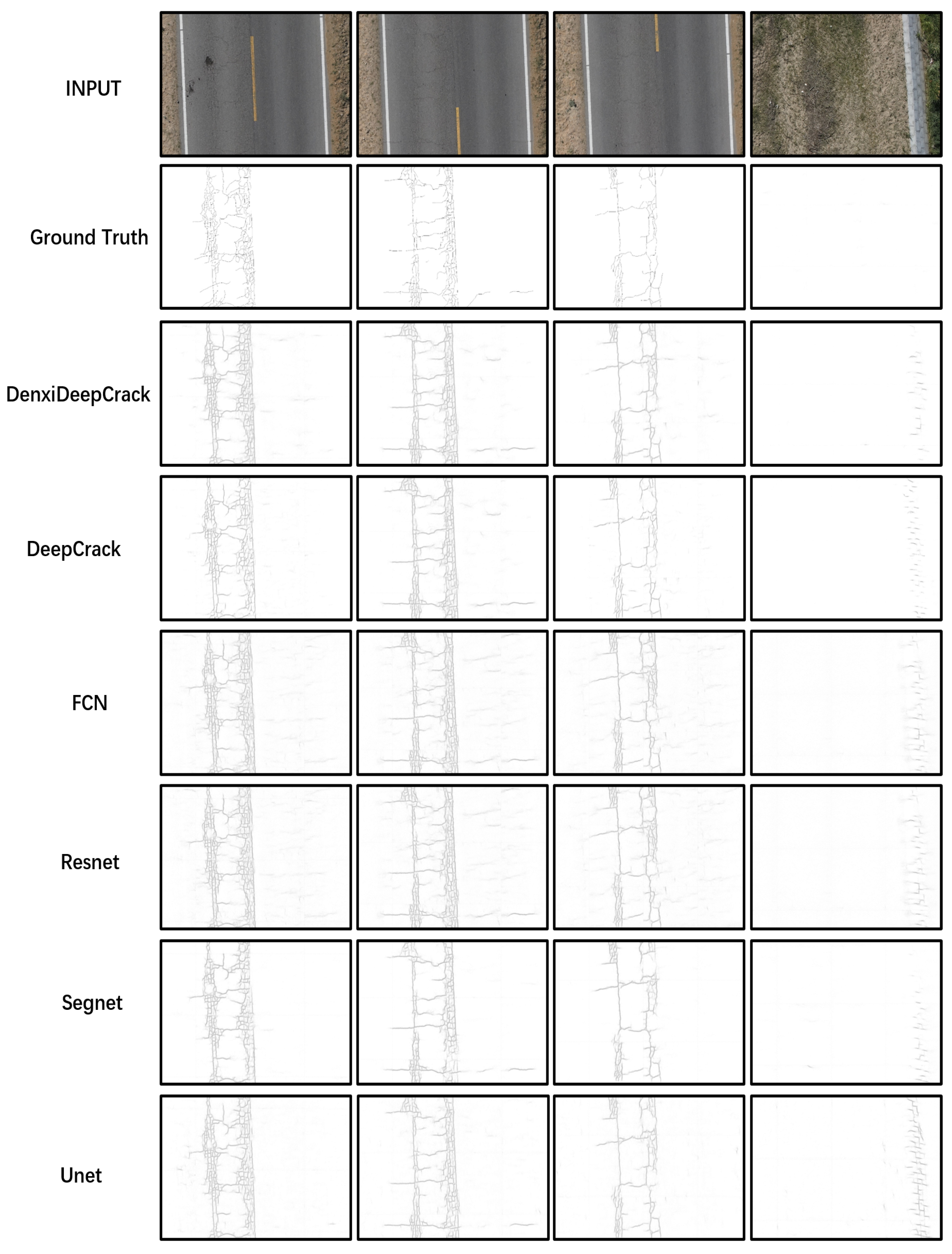
- A DenxiDeepCrack algorithm is proposed and experimentally demonstrated to be superior in crack detection based on UAV images.
- To be able to apply drone technology to crack detection, we manually labeled a dataset based on drone road pictures of cracks.
2. Background and Related Works
3. Proposed Approach
3.1. Vehicle Detection
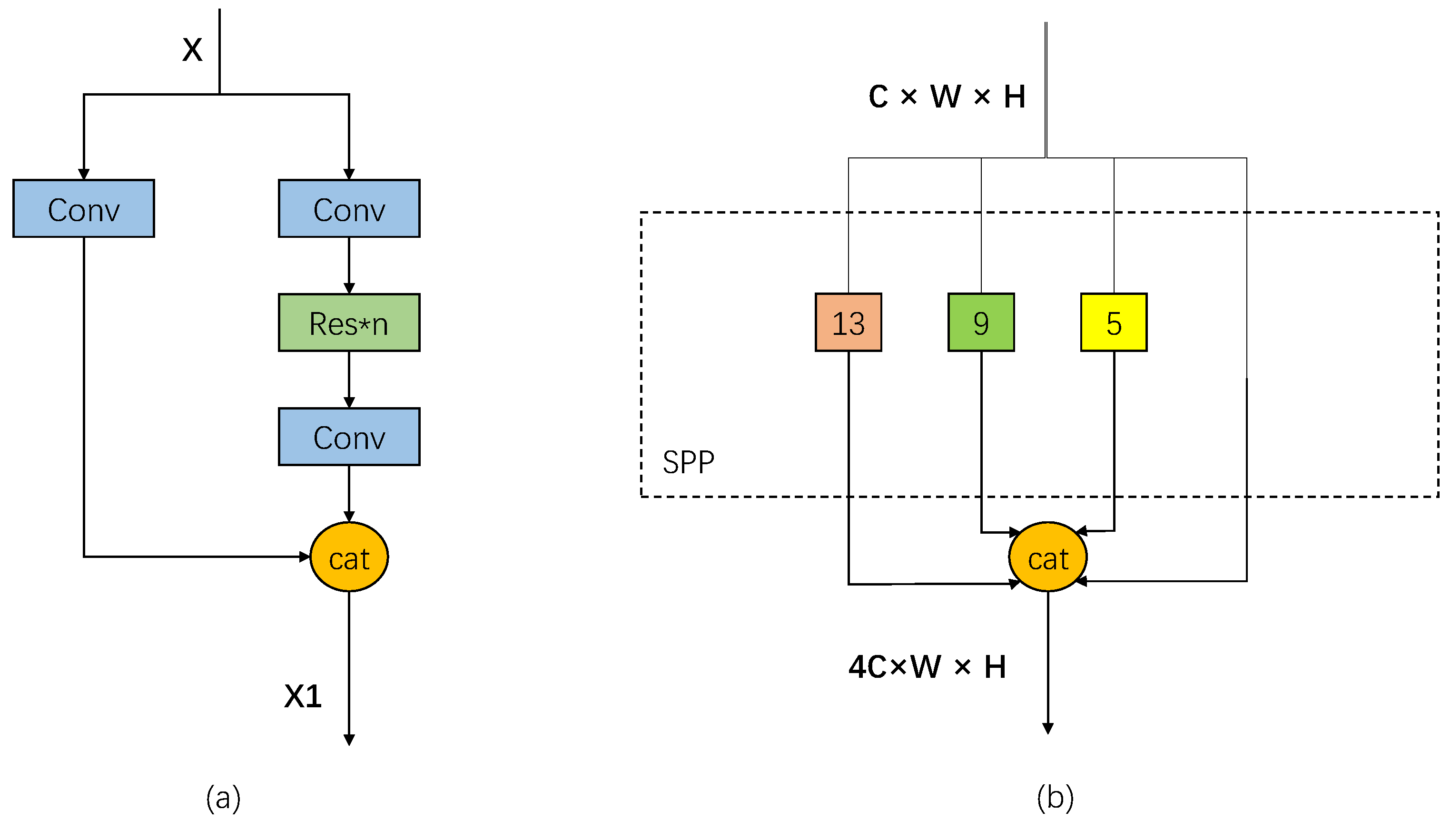
3.1.1. YOLOv4 Model
3.1.2. Loss
3.2. Feature-Based Image Stitching
3.2.1. Speeded Up Robust Features
3.2.2. Mathematical Setup
3.3. Crack Detection
3.3.1. DenxiDeepCrack
3.3.2. Loss
3.4. UCrack
4. Experimental Results
4.1. Vehicle Detection
4.1.1. Dataset
4.1.2. Training
4.1.3. Results
4.2. Feature-Based Image Stitching
4.3. Pixel-Level Crack Detection
4.3.1. Dataset
4.3.2. Training
4.3.3. Metrics
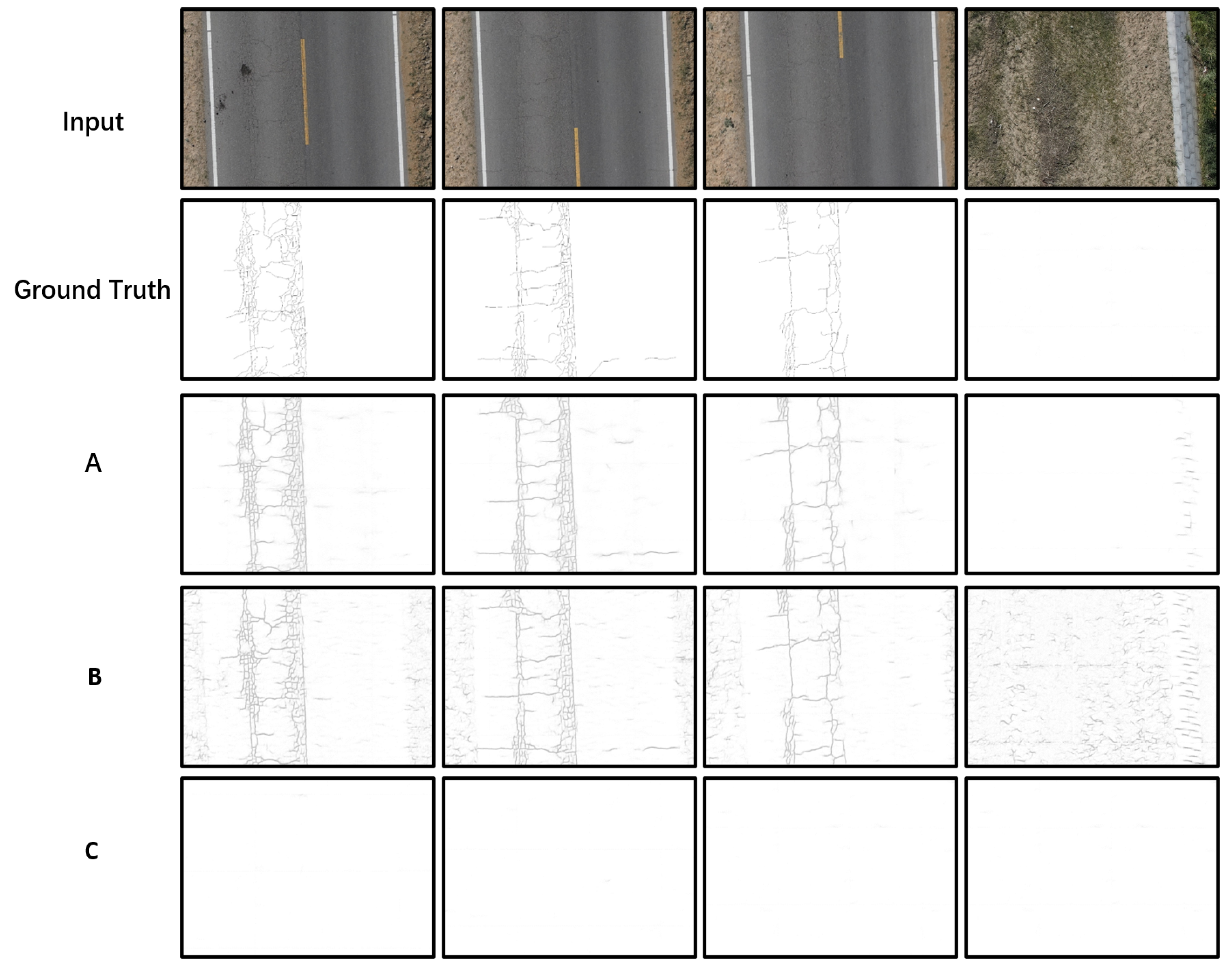
4.3.4. Results
5. Conclusions
Author Contributions
Funding
Institutional Review Board Statement
Informed Consent Statement
Data Availability Statement
Conflicts of Interest
References
- Broberg, P. Surface crack detection in welds using thermography. NDT E Int. 2013, 57, 69–73. [Google Scholar] [CrossRef]
- Soria, X.; Riba, E.; Sappa, Á.D. Dense Extreme Inception Network: Towards a Robust CNN Model for Edge Detection. In Proceedings of the IEEE Winter Conference on Applications of Computer Vision, WACV 2020, Snowmass Village, CO, USA, 1–5 March 2020; pp. 1912–1921. [Google Scholar]
- Guo, X.; Vavilov, V. Crack detection in aluminum parts by using ultrasound-excited infrared thermography. Infrared Phys. Technol. 2013, 61, 149–156. [Google Scholar] [CrossRef]
- Gunkel, C.; Stepper, A.; Müller, A.C.; Müller, C.H. Micro crack detection with Dijkstra’s shortest path algorithm. Mach. Vis. Appl. 2012, 23, 589–601. [Google Scholar] [CrossRef]
- Fujita, Y.; Hamamoto, Y. A robust automatic crack detection method from noisy concrete surfaces. Mach. Vis. Appl. 2011, 22, 245–254. [Google Scholar] [CrossRef]
- Glud, J.; Dulieu-Barton, J.; Thomsen, O.; Overgaard, L. Automated counting of off-axis tunnelling cracks using digital image processing. Compos. Sci. Technol. 2016, 125, 80–89. [Google Scholar] [CrossRef] [Green Version]
- Oliveira, H.; Correia, P.L. CrackIT—An image processing toolbox for crack detection and characterization. In Proceedings of the 2014 IEEE International Conference on Image Processing, ICIP 2014, Paris, France, 27–30 October 2014; pp. 798–802. [Google Scholar]
- Li, Q.; Liu, X. Novel Approach to Pavement Image Segmentation Based on Neighboring Difference Histogram Method. In Proceedings of the 2008 Congress on Image and Signal Processing, Sanya, China, 27–30 May 2008; Volume 2, pp. 792–796. [Google Scholar]
- Peng, L.; Chao, W.; Shuangmiao, L.; Baocai, F. Research on Crack Detection Method of Airport Runway Based on Twice-Threshold Segmentation. In Proceedings of the 2015 Fifth International Conference on Instrumentation and Measurement, Computer, Communication and Control (IMCCC), Qinhuangdao, China, 18–20 September 2015; pp. 1716–1720. [Google Scholar]
- Kapela, R.; Sniatala, P.; Turkot, A.; Rybarczyk, A.; Pozarycki, A.; Rydzewski, P.; Wyczalek, M.; Bloch, A. Asphalt surfaced pavement cracks detection based on histograms of oriented gradients. In Proceedings of the 22nd International Conference Mixed Design of Integrated Circuits & Systems, MIXDES 2015, Torun, Poland, 25–27 June 2015; pp. 579–584. [Google Scholar]
- Abdel-Qader, I.; Abudayyeh, O.; Kelly, M.E. Analysis of Edge-Detection Techniques for Crack Identification in Bridges. J. Comput. Civ. Eng. 2003, 17, 255–263. [Google Scholar] [CrossRef]
- Amhaz, R.; Chambon, S.; Idier, J.; Baltazart, V. Automatic Crack Detection on Two-Dimensional Pavement Images: An Algorithm Based on Minimal Path Selection. IEEE Trans. Intell. Transp. Syst. 2016, 17, 2718–2729. [Google Scholar] [CrossRef] [Green Version]
- Yuan, Y.; Fang, J.; Lu, X.; Feng, Y. Remote Sensing Image Scene Classification Using Rearranged Local Features. IEEE Trans. Geosci. Remote Sens. 2019, 57, 1779–1792. [Google Scholar] [CrossRef]
- Wang, C.; Bai, X.; Wang, S.; Zhou, J.; Ren, P. Multiscale Visual Attention Networks for Object Detection in VHR Remote Sensing Images. IEEE Geosci. Remote Sens. Lett. 2019, 16, 310–314. [Google Scholar] [CrossRef]
- Fang, J.; Cao, X. GAN and DCN Based Multi-step Supervised Learning for Image Semantic Segmentation. In Proceedings of the Pattern Recognition and Computer Vision–First Chinese Conference, PRCV 2018, Guangzhou, China, 23–26 November 2018; Lecture Notes in Computer Science Part II. Springer: Cham, Switzerland, 2018; Volume 11257, pp. 28–40. [Google Scholar]
- Eisenbach, M.; Stricker, R.; Seichter, D.; Amende, K.; Debes, K.; Sesselmann, M.; Ebersbach, D.; Stoeckert, U.; Gross, H. How to get pavement distress detection ready for deep learning? A systematic approach. In Proceedings of the 2017 International Joint Conference on Neural Networks, IJCNN 2017, Anchorage, AK, USA, 14–19 May 2017; pp. 2039–2047. [Google Scholar]
- Zhang, L.; Yang, F.; Zhang, Y.D.; Zhu, Y.J. Road crack detection using deep convolutional neural network. In Proceedings of the 2016 IEEE International Conference on Image Processing, ICIP 2016, Phoenix, AZ, USA, 25–28 September 2016; pp. 3708–3712. [Google Scholar]
- Li, S.; Zhao, X. Automatic crack detection and measurement of concrete structure using convolutional encoder-decoder network. IEEE Access 2020, 8, 134602–134618. [Google Scholar] [CrossRef]
- Xu, X.; Zhao, M.; Shi, P.; Ren, R.; He, X.; Wei, X.; Yang, H. Crack Detection and Comparison Study Based on Faster R-CNN and Mask R-CNN. Sensors 2022, 22, 1215. [Google Scholar] [CrossRef] [PubMed]
- Fan, Z.; Wu, Y.; Lu, J.; Li, W. Automatic Pavement Crack Detection Based on Structured Prediction with the Convolutional Neural Network. arXiv 2018, arXiv:1802.02208. [Google Scholar]
- Chen, F.; Jahanshahi, M.R. ARF-Crack: Rotation invariant deep fully convolutional network for pixel-level crack detection. Mach. Vis. Appl. 2020, 31, 47. [Google Scholar] [CrossRef]
- Nguyen, N.H.T.; Perry, S.W.; Bone, D.; Le, H.T.; Nguyen, T.T. Two-stage convolutional neural network for road crack detection and segmentation. Expert Syst. Appl. 2021, 186, 115718. [Google Scholar] [CrossRef]
- Sekar, A.; Perumal, V. Automatic road crack detection and classification using multi-tasking faster RCNN. J. Intell. Fuzzy Syst. 2021, 41, 6615–6628. [Google Scholar] [CrossRef]
- Badrinarayanan, V.; Kendall, A.; Cipolla, R. SegNet: A Deep Convolutional Encoder-Decoder Architecture for Image Segmentation. IEEE Trans. Pattern Anal. Mach. Intell. 2017, 39, 2481–2495. [Google Scholar] [CrossRef]
- Zou, Q.; Zhang, Z.; Li, Q.; Qi, X.; Wang, Q.; Wang, S. DeepCrack: Learning Hierarchical Convolutional Features for Crack Detection. IEEE Trans. Image Process. 2019, 28, 1498–1512. [Google Scholar] [CrossRef]
- Zhang, K.; Zhang, Y.; Cheng, H. CrackGAN: Pavement Crack Detection Using Partially Accurate Ground Truths Based on Generative Adversarial Learning. IEEE Trans. Intell. Transp. Syst. 2021, 22, 1306–1319. [Google Scholar] [CrossRef]
- Munawar, H.S.; Hammad, A.W.; Haddad, A.; Soares, C.A.P.; Waller, S.T. Image-based crack detection methods: A review. Infrastructures 2021, 6, 115. [Google Scholar] [CrossRef]
- Mohan, A.; Poobal, S. Crack detection using image processing: A critical review and analysis. Alex. Eng. J. 2018, 57, 787–798. [Google Scholar] [CrossRef]
- Redmon, J.; Farhadi, A. YOLOv3: An Incremental Improvement. arXiv 2018, arXiv:1804.02767. [Google Scholar]
- Bochkovskiy, A.; Wang, C.; Liao, H.M. YOLOv4: Optimal Speed and Accuracy of Object Detection. arXiv 2020, arXiv:2004.10934. [Google Scholar]
- Lowe, D.G. Distinctive Image Features from Scale-Invariant Keypoints. Int. J. Comput. Vis. 2004, 60, 91–110. [Google Scholar] [CrossRef]
- Bay, H.; Tuytelaars, T.; Gool, L.V. SURF: Speeded Up Robust Features. In Proceedings of the Computer Vision—ECCV 2006, 9th European Conference on Computer Vision, Graz, Austria, 7–13 May 2006; Lecture Notes in Computer Science Part I. Leonardis, A., Bischof, H., Pinz, A., Eds.; Springer: Berlin/Heidelberg, Germany, 2006; Volume 3951, pp. 404–417. [Google Scholar]
- Yang, F.; Deng, Z.S.; Fan, Q.H. A method for fast automated microscope image stitching. Micron 2013, 48, 17–25. [Google Scholar] [CrossRef]
- Zaragoza, J.; Chin, T.; Tran, Q.; Brown, M.S.; Suter, D. As-Projective-As-Possible Image Stitching with Moving DLT. IEEE Trans. Pattern Anal. Mach. Intell. 2014, 36, 1285–1298. [Google Scholar] [PubMed] [Green Version]
- Russell, B.C.; Torralba, A.; Murphy, K.P.; Freeman, W.T. LabelMe: A Database and Web-Based Tool for Image Annotation. Int. J. Comput. Vis. 2008, 77, 157–173. [Google Scholar] [CrossRef]
- Du, D.; Zhang, Y.; Wang, Z.; Wang, Z.; Song, Z.; Liu, Z.; Bo, L.; Shi, H.; Zhu, R.; Kumar, A.; et al. VisDrone-DET2019: The Vision Meets Drone Object Detection in Image Challenge Results. In Proceedings of the 2019 IEEE/CVF International Conference on Computer Vision Workshops, ICCV Workshops 2019, Seoul, Korea, 27–28 October 2019; pp. 213–226. [Google Scholar]
- Zou, Q.; Cao, Y.; Li, Q.; Mao, Q.; Wang, S. CrackTree: Automatic crack detection from pavement images. Pattern Recognit. Lett. 2012, 33, 227–238. [Google Scholar] [CrossRef]


| Dataset | Num | Car | People | Van | Truck | Motor | Bicycle | Tricycle | Awning-Tricycle | Bus |
|---|---|---|---|---|---|---|---|---|---|---|
| Training dataset | 5176 | 115,895 | 22,441 | 17,470 | 10,944 | 23,717 | 7860 | 4186 | 2565 | 4623 |
| Validation dataset | 1295 | 28,972 | 5500 | 7486 | 1931 | 5930 | 2620 | 626 | 681 | 1303 |
| Input | Batch Size | Learning Rate | Momentum | Decay | Iterations |
|---|---|---|---|---|---|
| 416 × 416 | 64 | 0.001 | 0.900 | 0.0005 | 15,000 |
| Method | Car | Van | Truck |
|---|---|---|---|
| Artificial | 32 | 6 | 27 |
| YOLOv4 | 33 | 7 | 27 |
| Method | ODS | OIS | AP |
|---|---|---|---|
| A | 0 | 0 | 0 |
| B | 0.175 | 0.191 | 0.073 |
| C | 0.614 | 0.64 | 0.632 |
| Method | ODS | OIS | AP |
|---|---|---|---|
| DenxiDeepcrack | 0.614 | 0.64 | 0.632 |
| Deepcrack | 0.468 | 0.51 | 0.417 |
| Segnet | 0.453 | 0.512 | 0.405 |
| Unet | 0.352 | 0.413 | 0.355 |
| Resnet | 0.452 | 0.515 | 0.413 |
| Fcn | 0.351 | 0.359 | 0.372 |
Publisher’s Note: MDPI stays neutral with regard to jurisdictional claims in published maps and institutional affiliations. |
© 2022 by the authors. Licensee MDPI, Basel, Switzerland. This article is an open access article distributed under the terms and conditions of the Creative Commons Attribution (CC BY) license (https://creativecommons.org/licenses/by/4.0/).
Share and Cite
Li, Y.; Ma, J.; Zhao, Z.; Shi, G. A Novel Approach for UAV Image Crack Detection. Sensors 2022, 22, 3305. https://doi.org/10.3390/s22093305
Li Y, Ma J, Zhao Z, Shi G. A Novel Approach for UAV Image Crack Detection. Sensors. 2022; 22(9):3305. https://doi.org/10.3390/s22093305
Chicago/Turabian StyleLi, Yanxiang, Jinming Ma, Ziyu Zhao, and Gang Shi. 2022. "A Novel Approach for UAV Image Crack Detection" Sensors 22, no. 9: 3305. https://doi.org/10.3390/s22093305
APA StyleLi, Y., Ma, J., Zhao, Z., & Shi, G. (2022). A Novel Approach for UAV Image Crack Detection. Sensors, 22(9), 3305. https://doi.org/10.3390/s22093305