
An Anisotropic Velocity Model for Microseismic Events Localization in Tunnels
1
School of Information Engineering, Southwest University of Science and Technology, Mianyang 621000, China
2
School of Control and Mechanical, Tianjin Chengjian University, Tianjin 300384, China
3
School of Automation and Information Engineering, Sichuan University of Science and Engineering, Zigong 643000, China
*
Author to whom correspondence should be addressed.
Sensors 2023, 23(10), 4670; https://doi.org/10.3390/s23104670
Submission received: 4 April 2023
/
Revised: 6 May 2023
/
Accepted: 9 May 2023
/
Published: 11 May 2023
(This article belongs to the Section Environmental Sensing)
Abstract
:The velocity model is one of the main factors affecting the accuracy of microseismic event localization. This paper addresses the issue of the low accuracy of microseismic event localization in tunnels and, combined with active-source technology, proposes a “source–station” velocity model. The velocity model assumes that the velocity from the source to each station is different, and it can greatly improve the accuracy of the time-difference-of-arrival algorithm. At the same time, for the case of multiple active sources, the MLKNN algorithm was selected as the velocity model selection method through comparative testing. The results of numerical simulation and laboratory tests in the tunnel showed that the average location accuracy of the “source–station” velocity model was improved compared with that of the isotropic velocity and sectional velocity models, with numerical simulation experiments improving accuracy by 79.82% and 57.05% (from 13.28 m and 6.24 m to 2.68 m), and laboratory tests in the tunnel improving accuracy by 89.26% and 76.33% (from 6.61 m and 3.00 m to 0.71 m). The results of the experiments showed that the method proposed in this paper can effectively improve the location accuracy of microseismic events in tunnels.
1. Introduction
The construction and maintenance of ultra-deep-buried tunnels pose significant engineering and technical challenges [1,2]. Rockburst is among the pivotal factors that impact heavily on the safety of deep-buried tunnels. It can result in injuries to workers, damage to equipment, and prolongation of construction time, and in severe cases, it can even trigger earthquakes [3,4,5]. Hence, it is imperative to monitor and provide early warning systems for rockburst events in tunnels. Microseismic monitoring technology is an essential tool for the early detection and monitoring of rockbursts [6]. Unlike other monitoring technologies, microseismic monitoring technology is capable of describing the spatiotemporal distribution of microseismic events in the monitored area. Therefore, the precise location of microseismic events is of utmost importance for most of the rockburst prediction methods based on microseismic monitoring, which are currently reliant on the statistical features of these events [7,8,9].
Tunnel engineering construction projects typically follow a linear path, and microseismic events frequently occur in proximity to the tunnel face; most occur beyond the scope of the sensor array. Thus, compared to conventional microseismic monitoring techniques, locating microseismic events in tunnel engineering is challenging [10,11]. In microseismic event localization, the commonly used methods are based on interferometry and time difference of arrival (TDOA) [12,13,14,15]. In tunnel engineering, TDOA-based methods are utilized the most frequently. However, due to the presence of large-scale openings (the already excavated part of the tunnel), the precision of the velocity model is low, leading to a lower location accuracy for the traditional TDOA-based algorithm. Scholars generally agree on this issue [16,17]. Numerous scholars have conducted comprehensive research on optimizing velocity models in tunnels; for example, Feng et al. [18] proposed a sectional velocity model, which considers that each group of sensors has the same velocity model and jointly solves microseismic event parameters using particle swarm algorithms until accuracy requirements are met. While this velocity model is particularly useful when the layer and tunnel are nearly perpendicular to one another, it is less effective when they form a certain angle or when the layer distribution is more complex, resulting in inconsistencies in sensor group velocity [19]. In addition, it is essentially still an SSH algorithm, and the introduction of more unknown parameters will lead to instability in the solution process and increase computational complexity [20,21]. In order to generate velocity models under different geological conditions, Ma et al. [22] proposed four different equivalent velocity models. However, these equivalent models cannot generate arbitrary complex velocity models. Peng et al. [23] proposed a 3D anisotropic velocity model based on the grid, which fully considers the impact of the excavation area when establishing the tunnel velocity model. It sets the velocity model of the excavation area to 340 m/s and the velocity of other areas to be consistent, and it uses block location (BL) to determine the approximate position of microseismic events. It then uses the improved nonlinear iterative particle swarm optimization (NPSO) algorithm to obtain the optimal solution. The aforementioned methods can achieve good results to a certain extent, but when the local geological structure is complex, it is often difficult to obtain desirable efficiency and results.
As is widely recognized, anisotropic velocity models can provide a more accurate representation of the propagation of microseismic events, although their development can be complicated [24]. In this paper, we present a “source–station” velocity model for microseismic event localization in tunnels, which takes into account that the velocity from the source to each station is different, making the velocity model anisotropic. Additionally, we assume that the propagation paths from similar sources to stations are similar, meaning that they can share the same velocity model. To exploit this assumption, an active-source array was deployed near the tunnel face, and a classification algorithm was used to select the active source closest to the microseismic event for location purposes.
The key contributions of this paper are as follows: (1) By combining active-source technology with the assumption that similar sources have similar propagation paths, we constructed the “source–station” velocity model. (2) The “source–station” velocity model allows for the omission of wave-type discrimination; this not only simplifies the computation process but also enhances the precision of localization. (3) We propose a method for selecting velocity models in the presence of multiple active sources.
The second part of the paper delves into the details of the “source–station” velocity model and explains the need for selecting velocity models when multiple active sources are involved. In the third part, we conduct numerical simulations experiments and laboratory tests in a tunnel environment to validate the accuracy of our proposed velocity model. We compare the results of these experiments with those obtained using isotropic velocity models and sectional velocity models. Additionally, we compare the accuracy of different velocity model selection methods and determine that the MLKNN algorithm is the best choice for selecting velocity models. The last section concludes the paper.
2. Methodologies
2.1. Location Method Based on Arrival-Time Theory
Microseismic events localization based on arrival-time theory is the most widely used location method. The TDOA algorithm determines the parameters of the microseismic events by calculating the residual between the observed arrival time and the theoretical arrival time [25]. Suppose that S (x0, y0, z0, t0) represents the source parameters of the microseismic event, where (x0, y0, z0) represents the spatial location of the source S and t0 represents the initiation time of source S, Ti (xi, yi, zi, ti) is the i-th station used to record the microseismic events, whose position (xi, yi, zi) is known, and the arrival time ti can be obtained through the arrival-time picking algorithm. The residual of station i can be described with Equation (1), where represents the observed travel time from source to station i, while represents the theoretical travel time from source to station i.
Suppose the velocity is isotropic, and the velocity value is v, can be expressed as:
where represents the distance between the source S and the station i:
By eliminating the simultaneous equation of all station residuals (Equation (1)), Equation (5) can be derived as follows:
In Equation (5), f represents the absolute value of the sum of the time residuals between the observation time and the calculated time at all stations (L1 norm), N represents the number of sensors, and n represents the norm (usually 1 or 2, related to the choice of the L1 or L2 norm). When the number of data points was limited, n = 2 was too sensitive to input errors. Therefore, in subsequent calculations in this paper, n = 1 [26].
As described in the principle of the arrival-time-difference location algorithm, Equation (5) uses the velocity from the source to the station, and, thus, the velocity model is one of the key factors affecting the accuracy of the location. Previous research has also confirmed that events outside the station are more sensitive to velocity model errors, and microseismic events in tunnels usually occur outside the station range [27]. Therefore, for the location of microseismic events in tunnels, an accurate velocity model is crucial.
2.2. “Source–Station” Velocity Model in a Tunnel
As shown in Figure 1, S0 represents the microseismic event to be located, and SS is the event induced by the nearby active source. The solid line (blue) in the figure represents the propagation path from SS to station Ti1, and the dotted line (red) represents the propagation path from S0 to station Ti1. We assumed that the propagation speeds Vi from SS to Ti are different, but due to the proximity of the two events, it can be assumed that the propagation paths of S0 and SS to each station were similar. Thus, when locating the unknown event S0, the velocity model Vi determined by the active source SS could be used. Based on this idea, this paper proposes a “source–station” velocity model based on active sources. In this velocity model, the velocities from the source to each station are different, and there are no constraints between the velocities. Therefore, the “source–station” velocity model can be considered an anisotropic velocity model.
Since the “source–station” velocity model is determined by the active source and only makes use of the information of the initial arriving wave, it is not necessary to distinguish the type (P wave, S wave, or other) of the initial arriving wave when locating the events nearby. This not only makes the calculation simpler and more convenient but also reduces the error caused by misjudging the type of the initial arriving wave and improves the localization accuracy.
2.3. Location Method Using the “Source–Station” Velocity Model
The source parameters of the active source SS are (xs, ys, zs, ts), and the source parameters of the event S0 to be located are (x0, y0, z0, t0), where ti is the time when station i is first triggered by the source, and the equation for locating event S0 can be expressed using the following equation:
In Equation (6), Ri0 represents the distance from event S0 to station i, which can be expressed by Equation (7), and Vi is the velocity model determined by the active source SS, which can be expressed by Equation (8):
In Equation (8), Ris represents the distance between event SS and station i and can be represented as follows:
If the active source is a controllable source, then its start time ts can be easily obtained through the microseismic events recording system.
If the active source is a source with an accurate start time that is difficult to directly obtain, such as a blast, human impact, etc., the TDOA method can be used to eliminate the effect of start time [28]. We can modify the residual function in Equation (6) to Equation (10), and Equation (11) can be used to express the “source–station” velocity model.
3. Experiments and Discussions
3.1. Numerical Simulation in the Tunnel
As shown in Figure 2, in this part of our research, we simulated the microseismic monitoring situation in the tunnel according to the method proposed by Feng et al. [18]. Eight stations were partially located within a circular tunnel with a diameter of twelve meters, and their coordinates are listed in Table 1. We placed five active sources on the tunnel face (working face in Figure 2). In order to better reflect the actual situation, one of the active sources was placed at the center of the tunnel face, which was used to establish the isotropic velocity model and the sectional velocity model. Their coordinates are listed in Table 2. One hundred microseismic events were randomly distributed after the tunnel face, assuming that the starting times of the active source and the microseismic events were both zero.
In the numerical simulation experiment, the modeling method proposed by Wang Yunhong et al. [29] was used for modeling. The source generation method used was the ellipsoid three-axis random generation method, and the time information generation method used was the 2.5D two-point fast ray tracing method. The distribution of the medium is shown by the red line in Figure 2, where the velocities of the medium were 4000 m/s, 4500 m/s, and 5000 m/s, and the velocity in the middle empty area was set to 340 m/s. Based on the coordinates of the microseismic sensors and of the 100 groups of microseismic events, and the velocities of each layer, the travel time information of the 100 groups of microseismic events was obtained. The positions and travel times of the random events can be found in Appendix A.
In this paper, a simulated annealing algorithm was used to locate 100 random events. The parameter settings for the simulated annealing algorithm were as follows: the initial search coordinate was (0, 0, 100), the upper limit of the search range for x and y was 10 and the lower limit was −10; the upper limit of the search range for z was 150 and the lower limit was 90; max iterations was 1000; the function tolerance was 1 × 10⁻⁶; and the temperature update function was an exponential temperature update. The results of the isotropic velocity model, the sectional velocity model, and the “source–station” velocity model were compared. The isotropic velocity model and the sectional velocity model were calculated using the active source Z, while the “source–station” velocity model was calculated using the active sources Z1–Z4. After the calculation, the isotropic velocity model was found to be 4695.84 m/s. The sectional velocity model used the method described in the literature. The two groups of velocities were 4613.00 m/s and 4902.64 m/s, respectively. In the “source–station” velocity model, all velocity models generated by the four active sources were brought into the calculation. The three velocity models are shown in Table 3.
As shown in Figure 3, under the same conditions, the location results using different velocity models indicated that the average location error using the isotropic velocity model was the largest, with an average location error of 13.28 m. The average location error of the sectional velocity model was 6.24 m, reducing the location error by 53%, which was similar to Feng’s results [18]. When using the “source–station” velocity model, the average location error was the smallest, at only 2.68 m, which was significantly smaller than the other two velocity models. It reduces the location error by 57.05% compared with the sectional velocity model and by 79.82% compared with the isotropic velocity model, greatly improving the localization accuracy.
3.2. Selection of the “Source–Station” Velocity Model
During prior tunnel simulation experiments, four groups of active sources were established, resulting in relatively favorable outcomes for the localization. However, the calculation of the velocity model was determined from the active source situated close to the microseismic event, based on the assumption of a “source–station” velocity model. As the actual event–source distance was unknown, a methodology to determine the velocity model from multiple active sources had to be employed. For this study, the model and data depicted in Figure 2 were utilized to compare and contrast the effectiveness of the MLKNN algorithm, the KNN algorithm, the SVM algorithm, and ANN for selecting the optimal velocity model.
The dataset consisted of 100 sets of microseismic events from eight stations, and their arrival times and velocity models. In this case, we needed to select the best velocity model for each microseismic event from four possible velocity models. For each microseismic event, the eight arrival times were used as data feature values, and the best velocity model, serving as the class label, exhibited the minimum localization error.
MLKNN used eight feature values, a label, and a second label (another velocity model with a localization error within 0.5 m, if it existed. If it did not exist, the second label was the same as the first one) as input, while KNN, SVM, and ANN used eight feature values and a label as input. Out of these 100 microseismic events, 50 sets of data were used for training, and 50 sets were used for testing. The comparison results are shown in Figure 4. MLKNN’s accuracy was 76%, KNN’s accuracy was 50%, SVM’s accuracy was 40%, and ANN’s accuracy was 38%. MLKNN exhibited a good selection performance with small sample sizes.
We compared the localization errors of the optimal velocity model selected by four different methods with the actual localization error of the best velocity model, as shown in Figure 5. In the simulation test, despite the lower selection accuracy rate of 76% with the MLKNN algorithm, the location error was still relatively close to the best match.
3.3. Tests in the Tunnel Laboratory
The laboratory tests were carried out in the tunnel laboratory of the School of Environment and Resources at Southwest University of Science and Technology in Mianyang, Sichuan Province. The tunnel laboratory is a brick and concrete structure which is approximately 2.6 m wide, 8 m long, and 3 m high, as shown in Figure 6. In the tests, a self-developed data collection device and 14 Hz omnidirectional sensors were used, with a geophone sensitivity of 80 V/m/s and a data sampling rate of 10 kHz. The microseismic events were realized through manual striking, and a geophone was placed near the striking point. The waveform of the geophone and each station were cross-correlated to calculate the travel time of the seismic wave.
In the test, seven geophones (T1–T7) were deployed, among which T1–T6 acted as station sensors and T7 was placed at the source striking point. There were four active-source events (Z1–Z4) that were used to generate the models, and 10 microseismic events (S1–S10) that were yet to be located. Most of the microseismic events in the tunnel occurred near the roof; therefore, all the microseismic events in the test were distributed outside the station range. The spatial distribution of the sensors and active sources are shown in Figure 7, and the coordinates of the stations, active sources, and microseismic events are listed in Table 4, Table 5 and Table 6.
Unlike the numerical simulation experiments, in order to increase fairness in the comparison, the isotropic velocity model, the sectional velocity model, and the “source–station” velocity model were generated by the same set of active sources, giving four sets of velocity models, as presented in Table 7. As drilling holes inside the tunnel laboratory is not allowed, geophones were attached to the laboratory walls using stone adhesives. This may have caused some coupling issues and, consequently, the velocities determined may not be entirely accurate. However, since both the active sources and the events were triggered under these conditions, the coupling issues did not affect the location results of the microseismic events.
A simulated annealing method was employed for the localization of ten microseismic events. The previous experiments had demonstrated the satisfactory performance of the MLKNN method in the selection process. With the implementation of MLKNN, we obtained the localization errors for different velocity models and the best-match localization errors for each velocity model. A comparison of these results is illustrated in Figure 8. From the figure, we can observe the same pattern as in the previous numerical simulation experiments. The isotropic velocity model had the largest localization error, followed by the sectional velocity model, and the “source–station” velocity model had the lowest.
It is worth noting that even though the average localization errors for the isotropic velocity model and the sectional velocity model were 6.61 m and 3.00 m, respectively, which may seem insignificant, such localization errors are still considered unacceptable when taking into account the overall size of the tunnel laboratory.
4. Conclusions
In this paper, a “source–station” velocity model for microseismic event localization in tunnels was proposed. This velocity model is an anisotropic velocity model, where the velocity from the source or event to each station is different and there is no constraint between them. The establishment of this velocity model was simple and effective. Additionally, since events that are close in distance have similar propagation paths (the idea of double-difference localization), when using this velocity model for microseismic event localization, it is not necessary to determine the phase type, but only to identify the arrival time, reducing the localization error caused by incorrect phase identification. Therefore, this method can accurately reflect the propagation law of microseismic waves from a certain point and its surrounding area to the rock cave and stations, and this velocity model is suitable for use in the localization of microseismic events in tunnels.
The results of the tunnel numerical simulation experiment showed that the adoption of the “source–station” velocity model significantly improved the accuracy of microseismic events localization compared with the isotropic velocity model and the sectional velocity model, with the average localization error reducing by 79.82% (from 13.28 m to 2.68 m) and by 57.05% (from 6.24 m to 2.68 m), respectively. In the laboratory experiment, the results were similar to the numerical simulation results, with the average localization error reducing by 89.26% (from 6.61 m to 0.71 m) and by 76.33% (from 3.00 m to 0.71 m), compared to the isotropic velocity model and the sectional velocity model, respectively. We also discussed the selection of velocity models in the case of multiple active sources, and the localization results showed that the selection of velocity models was necessary. Although the current selection method (MLKNN) still has deficiencies, based on the excellent performance of the “source–station” velocity model after incorporating the selection of velocity models based on the MLKNN algorithm into the process, the average localization error in the simulation results increased by 0.07 m from the best-match result, which was 2.02 m, and still better than the best results of the isotropic velocity model and the sectional velocity model. In the laboratory test, the average localization error increased by 0.27 m from the best result, which was 0.44 m, and was also better than the best results of the isotropic velocity model and the sectional velocity model.
In the current approaches to locating microseismic events in tunnels, the “source–station” velocity model and the multisource selection method based on the MLKNN algorithm are reliable and effective. This method is also applicable to microseismic monitoring scenarios where the stations are far from the microseismic events.
The establishment and application of the “source–station” velocity model in practical engineering can be seen in [30], but due to construction periods and conditions, it is currently not possible to verify the selection of the “source–station” velocity model through field testing. In future work, the authors will continue to search for relevant experimental conditions to improve the experimental results. Additionally, the method of selecting the velocity model when there are multiple active sources will be further optimized to improve the accuracy of location of microseismic events in tunnels.
Author Contributions
Conceptualization, T.S. and S.W.; methodology, T.S.; software, T.S.; validation, S.W. and X.J.; formal analysis, X.T.; investigation, T.S.; resources, T.S.; data curation, S.W.; writing—original draft preparation, T.S.; writing—review and editing, X.J. and G.P.; visualization, S.W.; supervision, X.T.; project administration, T.S.; funding acquisition, T.S. All authors have read and agreed to the published version of the manuscript.
Funding
This research was funded by the Youth Science Foundation of the National Natural Science Foundation of China (grant number 41604153), the Youth Science Foundation of Sichuan Province (grant number 2022NSFSC1110), and the Doctoral Fund of Southwest University of Science and Technology (grant number 19zx7159).
Data Availability Statement
The data presented in this study are available on request from the corresponding author.
Acknowledgments
The authors would like to thank the School of Resources and Environment of Southwest University of Science and Technology, which provided the tunnel laboratory to enable us to verify our proposed velocity model.
Conflicts of Interest
The authors declare no conflict of interest.
Appendix A

Table A1.
Location and Travel Times of the 100 Microseismic Events.
| Events | Location (m) | Travel Time of the Events (ms) | |||||||||
|---|---|---|---|---|---|---|---|---|---|---|---|
| x | y | z | 1 | 2 | 3 | 4 | 5 | 6 | 7 | 8 | |
| 1 | 7 | 5 | 102 | 21.7314 | 22.1966 | 22.4316 | 21.1734 | 12.2387 | 12.6283 | 12.9879 | 15.8662 |
| 2 | 9 | 4 | 120 | 25.0277 | 25.4568 | 25.7069 | 24.4018 | 15.5361 | 15.8796 | 16.2307 | 19.0641 |
| 3 | −5 | 1 | 102 | 21.7485 | 22.348 | 22.1797 | 21.0686 | 12.2654 | 12.8606 | 12.6022 | 15.6615 |
| 4 | 10 | −5 | 120 | 25.179 | 25.4672 | 25.7448 | 24.2795 | 15.7501 | 15.8943 | 16.2837 | 18.9043 |
| 5 | 10 | 7 | 104 | 22.1385 | 22.5875 | 22.9144 | 21.6424 | 12.6679 | 13.0328 | 13.5249 | 16.3751 |
| 6 | −8 | −3 | 103 | 22.0465 | 22.6259 | 22.3604 | 21.2281 | 12.6253 | 13.1861 | 12.7821 | 15.7884 |
| 7 | 6 | 2 | 114 | 23.9186 | 24.3584 | 24.5356 | 23.2411 | 14.4221 | 14.7784 | 15.0341 | 17.8793 |
| 8 | −10 | 7 | 116 | 24.3075 | 25.051 | 24.7627 | 23.8172 | 14.8213 | 15.6106 | 15.2003 | 18.4344 |
| 9 | 4 | 9 | 110 | 23.1404 | 23.7173 | 23.8401 | 22.7059 | 13.6209 | 14.1783 | 14.3582 | 17.3952 |
| 10 | −2 | 5 | 103 | 21.8648 | 22.4811 | 22.4146 | 21.3231 | 12.3447 | 12.9668 | 12.8652 | 15.959 |
| 11 | 4 | −9 | 110 | 23.4211 | 23.7173 | 23.8401 | 22.3828 | 14.036 | 14.1783 | 14.3582 | 16.9611 |
| 12 | −10 | 6 | 124 | 25.7577 | 26.4702 | 26.2028 | 25.2185 | 16.2653 | 17.0021 | 16.6326 | 19.8187 |
| 13 | 4 | 1 | 108 | 22.8252 | 23.2769 | 23.4028 | 22.1218 | 13.3304 | 13.7018 | 13.889 | 16.7483 |
| 14 | −10 | −3 | 102 | 21.9052 | 22.518 | 22.1829 | 21.0916 | 12.5079 | 13.1186 | 12.6071 | 15.652 |
| 15 | 6 | −4 | 106 | 22.5803 | 22.9166 | 23.1094 | 21.699 | 13.1478 | 13.3436 | 13.6324 | 16.3116 |
| 16 | 0 | 2 | 103 | 21.8892 | 22.4219 | 22.4219 | 21.2335 | 12.3826 | 12.8764 | 12.8764 | 15.8513 |
| 17 | 4 | 4 | 114 | 23.8811 | 24.3806 | 24.4988 | 23.2717 | 14.3672 | 14.8106 | 14.9812 | 17.9114 |
| 18 | 4 | −9 | 109 | 23.2425 | 23.5364 | 23.6606 | 22.2011 | 13.8612 | 13.9987 | 14.1813 | 16.7797 |
| 19 | −8 | −7 | 101 | 21.7992 | 22.3108 | 22.0397 | 20.832 | 12.4454 | 12.9015 | 12.4853 | 15.3735 |
| 20 | −3 | 10 | 119 | 24.7717 | 25.4542 | 25.3701 | 24.3522 | 15.249 | 15.9509 | 15.8324 | 19.0015 |
| 21 | −10 | 7 | 109 | 23.0419 | 23.8033 | 23.4936 | 22.5717 | 13.5638 | 14.3897 | 13.9353 | 17.2003 |
| 22 | −3 | 6 | 102 | 21.6832 | 22.3343 | 22.2335 | 21.1832 | 12.1633 | 12.8398 | 12.6851 | 15.8273 |
| 23 | 7 | 10 | 122 | 25.3516 | 25.892 | 26.0825 | 24.9052 | 15.8428 | 16.3432 | 16.6082 | 19.5938 |
| 24 | 4 | 8 | 121 | 25.1378 | 25.6928 | 25.803 | 24.6393 | 15.6159 | 16.1375 | 16.2918 | 19.2977 |
| 25 | 2 | 5 | 122 | 25.3168 | 25.8578 | 25.9124 | 24.7297 | 15.7937 | 16.2954 | 16.3718 | 19.3561 |
| 26 | 9 | 0 | 122 | 25.4312 | 25.8064 | 26.052 | 24.6839 | 15.9549 | 16.2234 | 16.5659 | 19.3207 |
| 27 | 1 | −2 | 101 | 21.5969 | 22.0439 | 22.078 | 20.792 | 12.1316 | 12.4919 | 12.5447 | 15.3873 |
| 28 | 2 | −4 | 104 | 22.1876 | 22.5864 | 22.6522 | 21.3108 | 12.743 | 13.0313 | 13.1312 | 15.8982 |
| 29 | −1 | −5 | 110 | 23.2899 | 23.7259 | 23.6951 | 22.3938 | 13.843 | 14.191 | 14.1457 | 16.9599 |
| 30 | 4 | −2 | 114 | 23.9599 | 24.3695 | 24.4878 | 23.1568 | 14.4821 | 14.7945 | 14.9653 | 17.7596 |
| 31 | 7 | −2 | 113 | 23.8104 | 24.1739 | 24.3826 | 23.0017 | 14.3483 | 14.5927 | 14.895 | 17.6247 |
| 32 | 4 | −7 | 113 | 23.8971 | 24.23 | 24.3492 | 22.9318 | 14.4745 | 14.6743 | 14.8468 | 17.5147 |
| 33 | −9 | −5 | 108 | 23.0094 | 23.568 | 23.2858 | 22.129 | 13.6058 | 14.1322 | 13.7151 | 16.6772 |
| 34 | −8 | 10 | 105 | 22.2851 | 23.0749 | 22.8165 | 21.9296 | 12.7949 | 13.672 | 13.2854 | 16.5989 |
| 35 | −2 | 6 | 112 | 23.4951 | 24.1157 | 24.0554 | 22.9663 | 13.971 | 14.5912 | 14.5034 | 17.5965 |
| 36 | −1 | 10 | 107 | 22.5834 | 23.2582 | 23.2265 | 22.2043 | 13.0582 | 13.7636 | 13.7165 | 16.8862 |
| 37 | 3 | −5 | 124 | 25.8205 | 26.2112 | 26.2917 | 24.9366 | 16.3529 | 16.6443 | 16.7559 | 19.5169 |
| 38 | 8 | 9 | 111 | 23.3686 | 23.8829 | 24.1255 | 22.9232 | 13.8713 | 14.3357 | 14.6885 | 17.6367 |
| 39 | 2 | 10 | 114 | 23.8585 | 24.4767 | 24.5356 | 23.4467 | 14.3342 | 14.9493 | 15.0341 | 18.1253 |
| 40 | −10 | 2 | 100 | 21.4546 | 22.1572 | 21.8142 | 20.8272 | 12.0132 | 12.766 | 12.2358 | 15.426 |
| 41 | −1 | −6 | 102 | 21.8797 | 22.2924 | 22.2588 | 20.9335 | 12.4686 | 12.7756 | 12.724 | 15.4967 |
| 42 | 6 | −3 | 122 | 25.4416 | 25.8167 | 25.9806 | 24.6096 | 15.9695 | 16.2378 | 16.4667 | 19.2141 |
| 43 | −9 | 6 | 107 | 22.6643 | 23.4003 | 23.1152 | 22.1635 | 13.1808 | 13.9736 | 13.5503 | 16.787 |
| 44 | 2 | 5 | 111 | 23.3182 | 23.8638 | 23.9247 | 22.7505 | 13.7965 | 14.3078 | 14.3969 | 17.3914 |
| 45 | 6 | 3 | 111 | 23.3647 | 23.818 | 24.0007 | 22.7229 | 13.8655 | 14.2405 | 14.5076 | 17.3724 |
| 46 | −4 | 7 | 107 | 22.5955 | 23.2701 | 23.1431 | 22.1184 | 13.0767 | 13.7812 | 13.592 | 16.7596 |
| 47 | 6 | 3 | 124 | 25.7211 | 26.1801 | 26.341 | 25.0658 | 16.2142 | 16.6011 | 16.8242 | 19.698 |
| 48 | −8 | −9 | 111 | 23.6457 | 24.1255 | 23.8829 | 22.6359 | 14.278 | 14.6885 | 14.3357 | 17.1714 |
| 49 | 5 | 5 | 122 | 25.3351 | 25.8347 | 25.9712 | 24.7429 | 15.8195 | 16.263 | 16.4537 | 19.3841 |
| 50 | 9 | 6 | 107 | 22.6643 | 23.1152 | 23.4003 | 22.1266 | 13.1808 | 13.5503 | 13.9736 | 16.8317 |
| 51 | −4 | 6 | 122 | 25.3229 | 25.9593 | 25.8501 | 24.7763 | 15.8023 | 16.4371 | 16.2846 | 19.3883 |
| 52 | 9 | 5 | 119 | 24.8405 | 25.283 | 25.5354 | 24.2465 | 15.3471 | 15.7093 | 16.0649 | 18.9171 |
| 53 | 10 | −9 | 109 | 23.3245 | 23.5248 | 23.834 | 22.2741 | 13.9817 | 13.9814 | 14.4343 | 16.8982 |
| 54 | −10 | 0 | 112 | 23.6444 | 24.2919 | 23.9912 | 22.9351 | 14.1906 | 14.8459 | 14.4096 | 17.5073 |
| 55 | 1 | −9 | 118 | 24.8388 | 25.1938 | 25.2221 | 23.8283 | 15.4225 | 15.659 | 15.6992 | 18.3894 |
| 56 | 0 | 4 | 118 | 24.5927 | 25.1494 | 25.1494 | 23.9847 | 15.0713 | 15.5961 | 15.5961 | 18.6002 |
| 57 | 8 | −6 | 118 | 24.812 | 25.1103 | 25.3369 | 23.8818 | 15.3844 | 15.5406 | 15.8611 | 18.4907 |
| 58 | 5 | −4 | 121 | 25.2715 | 25.6454 | 25.7833 | 24.4104 | 15.805 | 16.0708 | 16.2642 | 19.0059 |
| 59 | −6 | −1 | 118 | 24.6837 | 25.2531 | 25.0827 | 23.9324 | 15.2017 | 15.7429 | 15.5013 | 18.5006 |
| 60 | −3 | −8 | 123 | 25.7144 | 26.1439 | 26.0628 | 24.7523 | 16.2776 | 16.622 | 16.5093 | 19.3013 |
| 61 | 9 | −9 | 118 | 24.9102 | 25.1512 | 25.4055 | 23.8873 | 15.5235 | 15.5987 | 15.9575 | 18.4951 |
| 62 | 2 | 5 | 108 | 22.7731 | 23.3202 | 23.3832 | 22.2116 | 13.252 | 13.7664 | 13.8599 | 16.8574 |
| 63 | −2 | 3 | 111 | 23.3337 | 23.9095 | 23.8485 | 22.7071 | 13.8196 | 14.3747 | 14.2854 | 17.3152 |
| 64 | 8 | 0 | 121 | 25.2358 | 25.6237 | 25.8442 | 24.4899 | 15.7545 | 16.0404 | 16.3492 | 19.1213 |
| 65 | 0 | −8 | 112 | 23.732 | 24.1082 | 24.1082 | 22.7393 | 14.3186 | 14.5802 | 14.5802 | 17.2989 |
| 66 | 5 | 9 | 117 | 24.4202 | 24.9773 | 25.1202 | 23.9614 | 14.9029 | 15.4285 | 15.6315 | 18.6407 |
| 67 | −6 | −9 | 109 | 23.262 | 23.7108 | 23.5248 | 22.2417 | 13.89 | 14.2549 | 13.9814 | 16.7797 |
| 68 | −7 | −7 | 100 | 21.6048 | 22.0997 | 21.8595 | 20.6322 | 12.2474 | 12.6781 | 12.3067 | 15.1746 |
| 69 | −10 | 9 | 123 | 25.5741 | 26.3288 | 26.0594 | 25.1252 | 16.0815 | 16.8775 | 16.5046 | 19.7479 |
| 70 | 5 | −1 | 112 | 23.589 | 23.9968 | 24.1476 | 22.8159 | 14.1094 | 14.4179 | 14.6376 | 17.4318 |
| 71 | 0 | 6 | 112 | 23.4912 | 24.0818 | 24.0818 | 22.9585 | 13.9653 | 14.5419 | 14.5419 | 17.5965 |
| 72 | −10 | −10 | 115 | 24.4243 | 24.9187 | 24.628 | 23.3987 | 15.0692 | 15.5008 | 15.0866 | 17.931 |
| 73 | −10 | −4 | 120 | 25.1571 | 25.7371 | 25.4594 | 24.3237 | 15.7192 | 16.2728 | 15.8833 | 18.8733 |
| 74 | −1 | 8 | 118 | 24.5792 | 25.2071 | 25.1787 | 24.0972 | 15.0518 | 15.6779 | 15.6377 | 18.7384 |
| 75 | −4 | −9 | 109 | 23.2425 | 23.6606 | 23.5364 | 22.2173 | 13.8612 | 14.1813 | 13.9987 | 16.7599 |
| 76 | 6 | 8 | 123 | 25.5183 | 26.045 | 26.2071 | 25.0117 | 16.0032 | 16.4845 | 16.7096 | 19.6776 |
| 77 | 10 | 10 | 115 | 24.1295 | 24.628 | 24.9187 | 23.6999 | 14.6455 | 15.0866 | 15.5008 | 18.426 |
| 78 | −7 | 8 | 119 | 24.8039 | 25.5136 | 25.3174 | 24.3305 | 15.2949 | 16.0343 | 15.7579 | 18.9545 |
| 79 | −4 | −2 | 108 | 22.8761 | 23.4057 | 23.2798 | 22.086 | 13.4069 | 13.8933 | 13.7062 | 16.6572 |
| 80 | 0 | −6 | 114 | 24.0347 | 24.4435 | 24.4435 | 23.1106 | 14.5907 | 14.9015 | 14.9015 | 17.6763 |
| 81 | 5 | 1 | 101 | 21.5677 | 21.9981 | 22.1682 | 20.8664 | 12.0859 | 12.4207 | 12.6837 | 15.51 |
| 82 | 1 | 3 | 116 | 24.2386 | 24.7673 | 24.7962 | 23.6 | 14.7216 | 15.2068 | 15.2483 | 18.2151 |
| 83 | 7 | −10 | 109 | 23.3089 | 23.5403 | 23.7571 | 22.2295 | 13.9589 | 14.0044 | 14.3224 | 16.8267 |
| 84 | −3 | 8 | 120 | 24.9499 | 25.603 | 25.5195 | 24.4663 | 15.4255 | 16.0853 | 15.9681 | 19.098 |
| 85 | −1 | −10 | 103 | 22.1932 | 22.5391 | 22.506 | 21.1065 | 12.8491 | 13.0549 | 13.0046 | 15.6566 |
| 86 | 1 | −9 | 109 | 23.2278 | 23.5685 | 23.5996 | 22.1919 | 13.8395 | 14.046 | 14.0917 | 16.7537 |
| 87 | 4 | 10 | 107 | 22.5986 | 23.1938 | 23.3205 | 22.2095 | 13.0813 | 13.6677 | 13.8559 | 16.9171 |
| 88 | 8 | 7 | 112 | 23.5497 | 24.0337 | 24.2741 | 23.0352 | 14.0516 | 14.4717 | 14.8204 | 17.7284 |
| 89 | −7 | 5 | 124 | 25.7186 | 26.3786 | 26.191 | 25.1444 | 16.2106 | 16.876 | 16.6163 | 19.7417 |
| 90 | 1 | −1 | 104 | 22.1187 | 22.5844 | 22.6173 | 21.3516 | 12.6375 | 13.0281 | 13.0782 | 15.9512 |
| 91 | −8 | −4 | 109 | 23.1473 | 23.706 | 23.4575 | 22.2994 | 13.7206 | 14.2478 | 13.8818 | 16.8526 |
| 92 | −10 | 9 | 102 | 21.7774 | 22.5927 | 22.2588 | 21.404 | 12.3103 | 13.231 | 12.724 | 16.0695 |
| 93 | 4 | −5 | 120 | 25.1052 | 25.4777 | 25.5891 | 24.2145 | 15.646 | 15.9091 | 16.0659 | 18.8013 |
| 94 | 9 | 6 | 111 | 23.3879 | 23.8409 | 24.1142 | 22.841 | 13.8999 | 14.2742 | 14.6721 | 17.5357 |
| 95 | 6 | −8 | 109 | 23.2297 | 23.5082 | 23.6944 | 22.2183 | 13.8424 | 13.9569 | 14.2309 | 16.8131 |
| 96 | 2 | −5 | 106 | 22.5732 | 22.9579 | 23.0222 | 21.6643 | 13.137 | 13.4058 | 13.5023 | 16.2459 |
| 97 | 1 | −9 | 122 | 25.5562 | 25.9167 | 25.944 | 24.5556 | 16.1301 | 16.3777 | 16.4158 | 19.1164 |
| 98 | 7 | 0 | 114 | 23.9571 | 24.3519 | 24.5586 | 23.2133 | 14.478 | 14.769 | 15.067 | 17.846 |
| 99 | −10 | −1 | 120 | 25.1017 | 25.7241 | 25.4463 | 24.3587 | 15.641 | 16.2548 | 15.8648 | 18.9214 |
| 100 | 3 | 6 | 104 | 22.0465 | 22.5957 | 22.6943 | 21.5279 | 12.5261 | 13.0454 | 13.1948 | 16.1965 |
References
- Ren, B.; Shen, Y.; Zhao, T.; Li, X. Deformation monitoring and remote analysis of ultra-deep underground space excavation. Undergr. Space 2023, 8, 30–44. [Google Scholar] [CrossRef]
- Zhu, H.; Yan, J.; Liang, W. Challenges and Development Prospects of Ultra-Long and Ultra-Deep Mountain Tunnels. Engineering 2019, 5, 384–392. [Google Scholar] [CrossRef]
- Si, X.; Peng, K.; Luo, S. Experimental Investigation on the Influence of Depth on Rockburst Characteristics in Circular Tunnels. Sensors 2022, 22, 3679. [Google Scholar] [CrossRef] [PubMed]
- Zhang, H.; Chen, L.; Chen, S.; Sun, J.; Yang, J. The Spatiotemporal Distribution Law of Microseismic Events and Rockburst Characteristics of the Deeply Buried Tunnel Group. Energies 2018, 11, 3257. [Google Scholar] [CrossRef]
- Zhang, R.; Gong, S.; Dou, L.; Cai, W.; Li, X.; Li, H.; Tian, X.; Ding, X.; Niu, J. Evaluation of Anti-Burst Performance in Mining Roadway Support System. Sensors 2023, 23, 931. [Google Scholar] [CrossRef]
- Zhou, Z.; Zhao, C.; Huang, Y. An Optimization Method for the Station Layout of a Microseismic Monitoring System in Underground Mine Engineering. Sensors 2022, 22, 4775. [Google Scholar] [CrossRef]
- Liu, X.; Zhang, S.; Wang, E.; Zhang, Z.; Wang, Y.; Yang, S. Multi-Index Geophysical Monitoring and Early Warning for Rockburst in Coalmine: A Case Study. Int. J. Environ. Res. Public Health 2023, 20, 392. [Google Scholar] [CrossRef]
- Lyu, P.; Bao, X.; Lyu, G.; Chen, X. Research on Fault Activation Law in Deep Mining Face and Mechanism of Rockburst Induced by Fault Activation. Adv. Civ. Eng. 2020, 2020, 8854467. [Google Scholar] [CrossRef]
- Sheng, G.; Yang, S.; Tang, X.G.; Guo, X. Arrival-time picking of microseismic events based on MSNet. Geophys. J. Soc. Explor. Geophys. 2022, 87, 57–71. [Google Scholar] [CrossRef]
- Wang, Z.G.; Li, J.; Li, B. Source location mechanism of microseismic monitoring using P-S waves and its effect analysis. Dyna 2022, 97, 39–45. [Google Scholar] [CrossRef]
- Zhang, H.; Ma, C.; Li, T. Quantitative Evaluation of the “Non-Enclosed” Microseismic Array: A Case Study in a Deeply Buried Twin-Tube Tunnel. Energies 2019, 12, 2006. [Google Scholar] [CrossRef]
- Wu, S.; Wang, Y. Least-squares interferometric migration of microseismic source location with a deblurring filter. Geophysics 2023, 88, L37–L52. [Google Scholar] [CrossRef]
- Wu, S.; Wang, Y.; Xie, F.; Chang, X. Crosscorrelation migration of microseismic source locations with hybrid imaging condition. Geophysics 2022, 87, KS17–KS31. [Google Scholar] [CrossRef]
- Wu, S.; Wang, Y.; Zheng, Y.; Chang, X. Microseismic source locations with deconvolution migration. Geophys. J. Int. 2018, 212, 2088–2115. [Google Scholar] [CrossRef]
- Wu, S.; Wang, Y.; Zhan, Y.; Chang, X. Automatic microseismic event detection by band-limited phase-only correlation. Phys. Earth Planet. Inter. 2016, 261, 3–16. [Google Scholar] [CrossRef]
- Wang, K.; Tang, C.A.; Ma, K.; Yu, G.; Zhang, S.; Peng, Y. Cross-related microseismic location based on improved particle swarm optimization and the double-difference location method of jointed coal rock mass. Waves Random Complex Media 2021, 1–24. [Google Scholar] [CrossRef]
- Peng, P.; Jiang, Y.; Wang, L.; He, Z. Microseismic Event Location by Considering the Influence of the Empty Area in an Excavated Tunnel. Sensors 2020, 20, 574. [Google Scholar] [CrossRef]
- Feng, G.; Feng, X.; Chen, B.; Xiao, Y.; Jiang, Q. Sectional velocity model for microseismic source location in tunnels. Tunn. Undergr. Space Technol. 2015, 45, 73–83. [Google Scholar] [CrossRef]
- Zhang, Z.; Arosio, D.; Hojat, A.; Zanzi, L. Designing the Expanded Microseismic Monitoring Network for an Unstable Rock Face in Northern Italy. Pure Appl. Geophys. 2022, 179, 1623–1644. [Google Scholar] [CrossRef]
- Feng, G.; Feng, X.; Chen, B.; Xiao, Y. Performance and feasibility analysis of two microseismic location methods used in tunnel engineering. Tunn. Undergr. Space Technol. 2017, 63, 183–193. [Google Scholar] [CrossRef]
- Jiang, H.; Wang, Z.; Zeng, X.; Lü, H.; Zhou, X.; Chen, Z. Velocity model optimization for surface microseismic monitoring via amplitude stacking. Appl. Geophys. 2016, 135, 317–327. [Google Scholar] [CrossRef]
- Ma, C.; Jiang, Y.; Li, T. Gravitational Search Algorithm for Microseismic Source Location in Tunneling: Performance Analysis and Engineering Case Study. Rock Mech. Rock Eng. 2019, 52, 3999–4016. [Google Scholar] [CrossRef]
- Peng, P.; Wang, L. Targeted location of microseismic events based on a 3D heterogeneous velocity model in underground mining. PLoS ONE 2019, 14, e0212881. [Google Scholar] [CrossRef]
- Feng, Q.; Han, L.; Pan, B.; Zhao, B. Microseismic Source Location Using Deep Reinforcement Learning. IEEE Trans. Geosci. Remote Sens. 2022, 60, 1–9. [Google Scholar] [CrossRef]
- Cong, S.; Wang, Y.; Cheng, J. Coal mine microseismic velocity model inversion based on first arrival time difference. Arab. J. Geosci. 2018, 12, 5. [Google Scholar] [CrossRef]
- Ge, M. Source location error analysis and optimization methods. J. Rock Mech. Geotech. Eng. 2012, 4, 1–10. [Google Scholar] [CrossRef]
- Dong, L.; Hu, Q.; Tong, X.; Liu, Y. Velocity-free MS/AE source location method for three-dimensional hole-containing structures. Engineering 2020, 6, 827–834. [Google Scholar] [CrossRef]
- Wu, S.; Wang, Y.; Liang, X. Time-Delay Estimation of Microseismic DAS Data Using Band-Limited Phase-Only Correlation. IEEE Trans. Geosci. Remote Sens. 2022, 61, 22477055. [Google Scholar] [CrossRef]
- Wang, Y.; Dong, R. Study on micro-seismic forward modeling in coalbed methane well hydraulic fracturing. Coal Sci. Technol. 2016, 44, 137–141. [Google Scholar]
- Shen, T. Research on Key Technologies for the Optimization of Microseismic Events Location Accuracy. Ph.D. Thesis, Chengdu University of Technology, Chengdu, China, 2019. [Google Scholar] [CrossRef]
Figure 1.
“Source–station” velocity model in tunnel. The solid black circle represents the location of the source, and the solid black pentagram represents the location of a microseismic event near the active source. The blue solid line represents the propagation path from the active source to the first station in group q, and the red dashed line represents the propagation path from the microseismic event to the corresponding station.
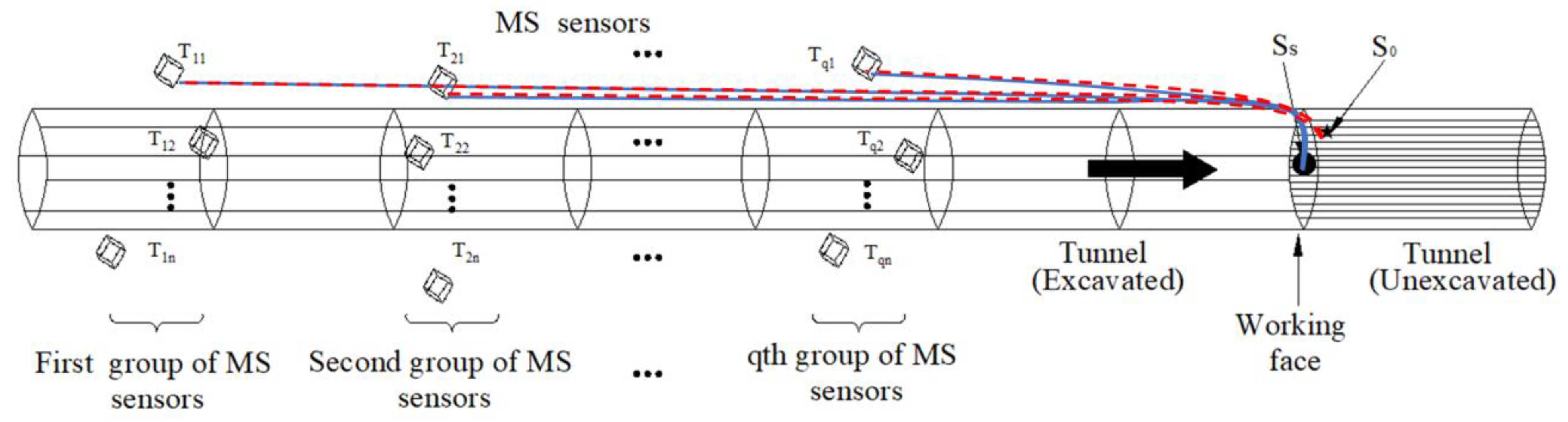
Figure 2.
Simulation of microseismic monitoring in a tunnel. The eight cubes represent eight stations, which were placed in two groups. The five solid red circles represent five active sources (Z and Z1–Z4), which were set on the tunnel face. Among the five active sources, four (Z1–Z4) were used to establish the “source–station” velocity model, and one (Z) was used to establish the isotropic velocity model and the sectional velocity model. One hundred microseismic events were randomly distributed in the black zone. The red line represents the layered structure of the medium in the numerical simulations.
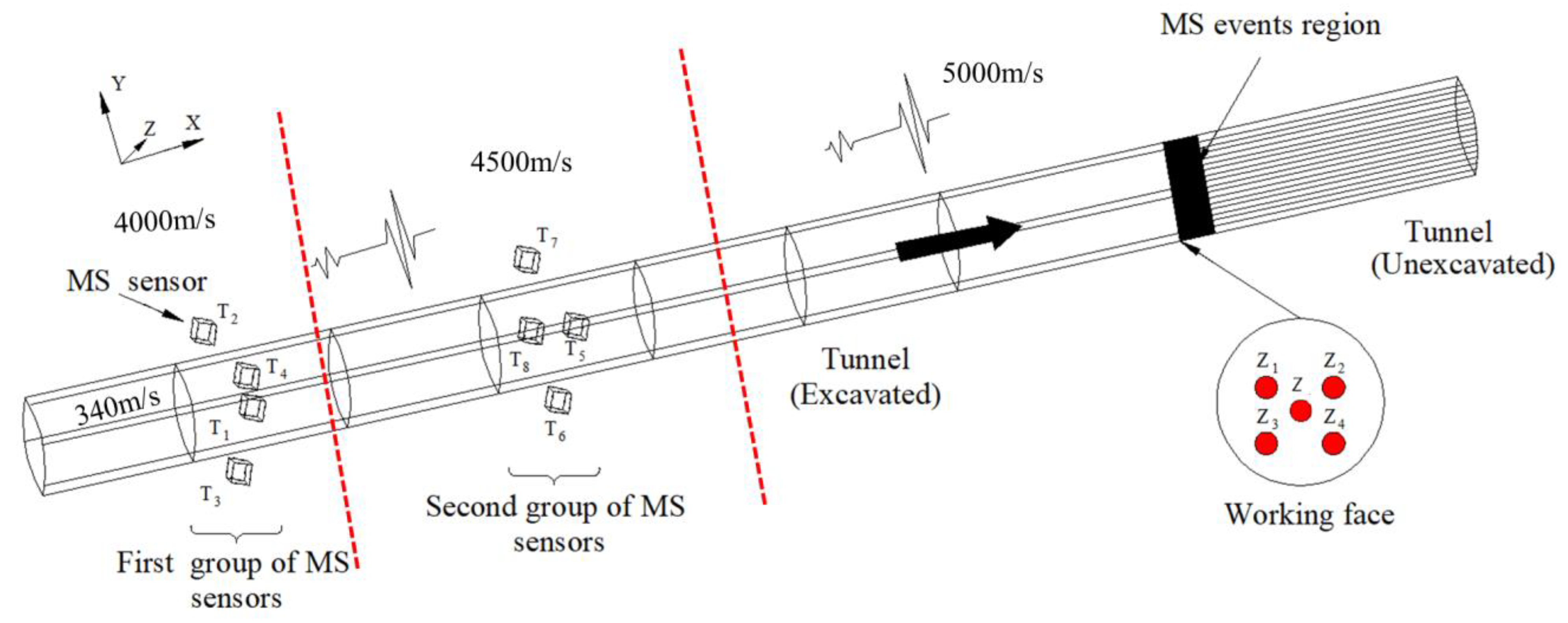
Figure 3.
Location errors with different velocity models.
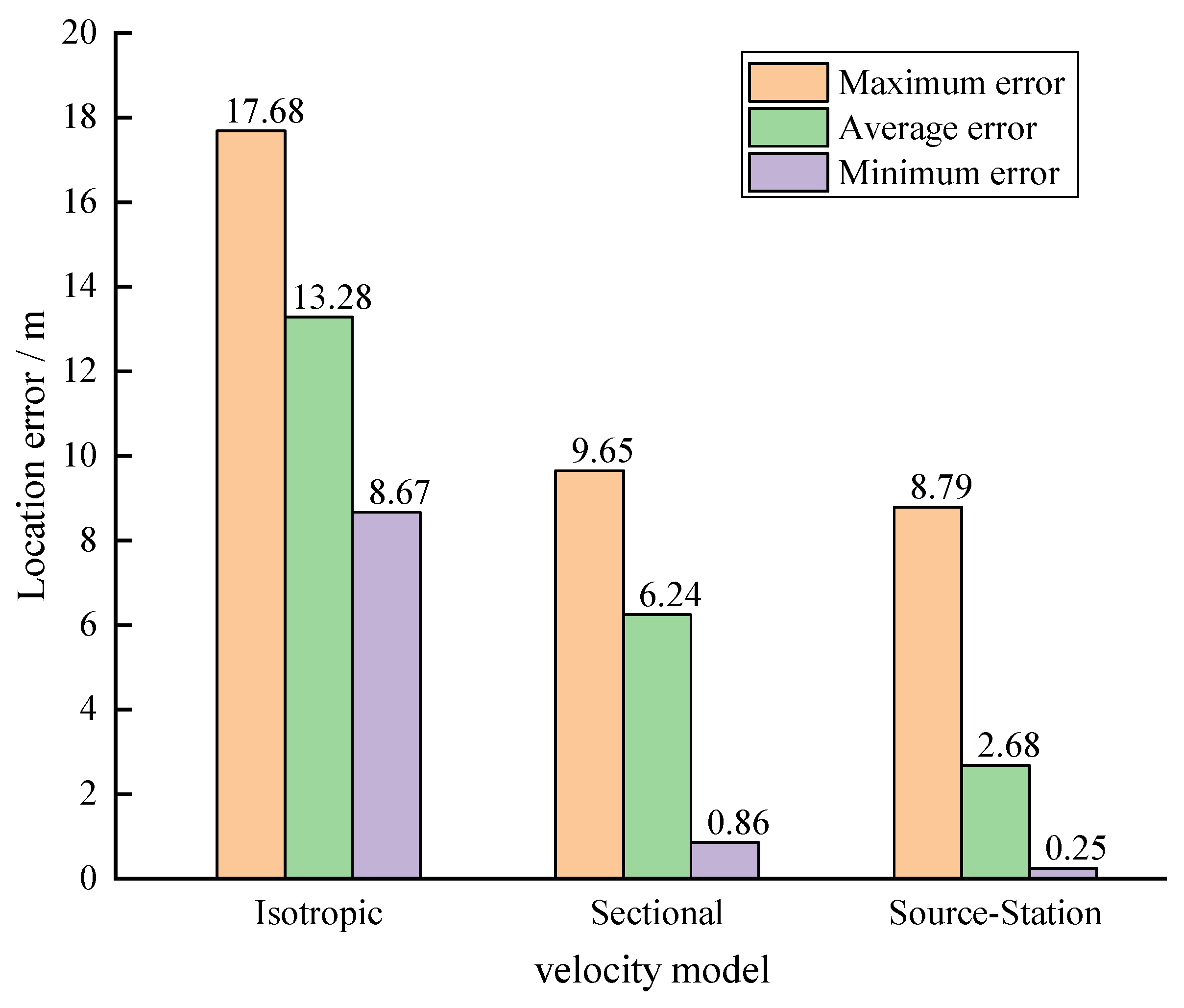
Figure 4.
Comparison results obtained by different selection methods.
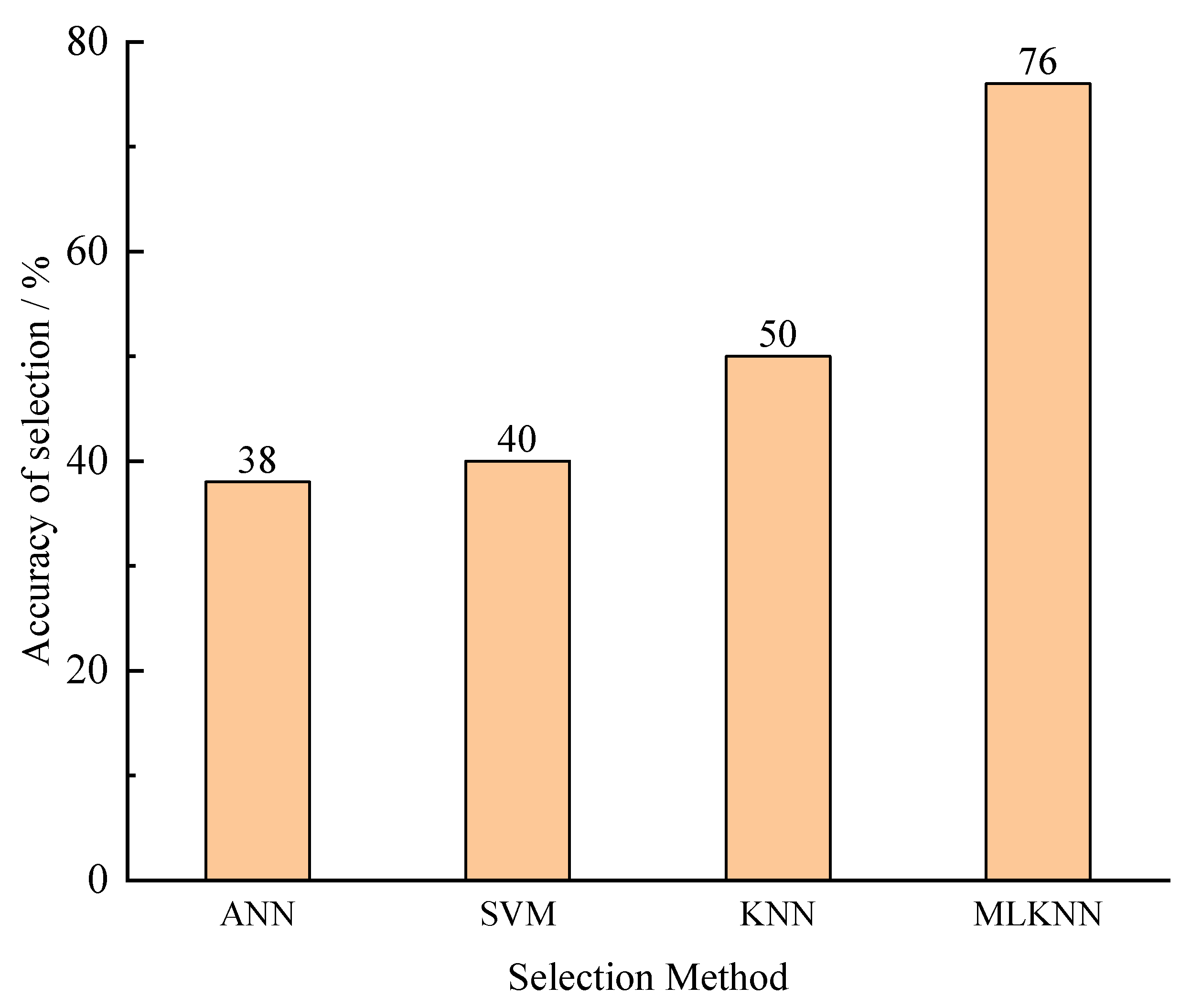
Figure 5.
Comparison of location errors for different velocity model selection methods. The best match was the velocity model that exhibited the minimum localization error during the experiment.
Figure 5.
Comparison of location errors for different velocity model selection methods. The best match was the velocity model that exhibited the minimum localization error during the experiment.
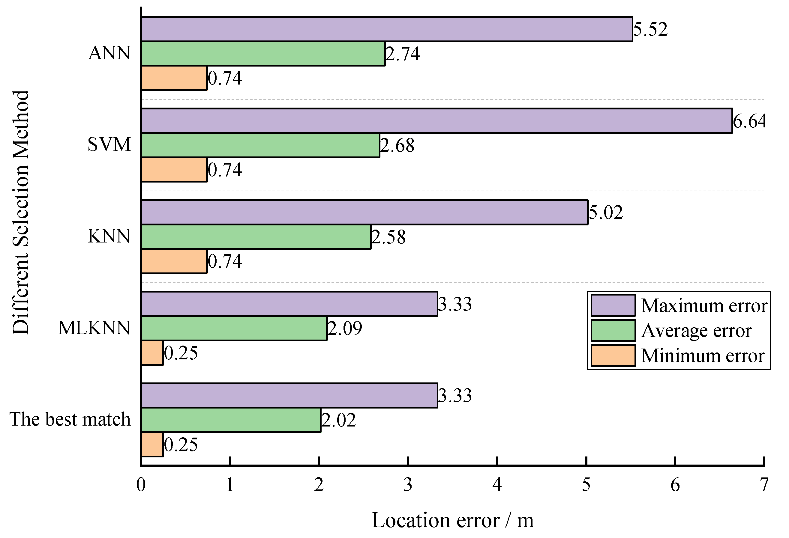
Figure 6.
The tunnel laboratory of the School of Environment and Resources at Southwest University of Science and Technology. (a) Tunnel laboratory appearance; (b) tunnel laboratory structure.
Figure 6.
The tunnel laboratory of the School of Environment and Resources at Southwest University of Science and Technology. (a) Tunnel laboratory appearance; (b) tunnel laboratory structure.

Figure 7.
Distribution of stations (MS sensors) and active sources in the tunnel laboratory. The black dots represent the stations (T1–T6), and the red dots represent the active sources.
Figure 7.
Distribution of stations (MS sensors) and active sources in the tunnel laboratory. The black dots represent the stations (T1–T6), and the red dots represent the active sources.
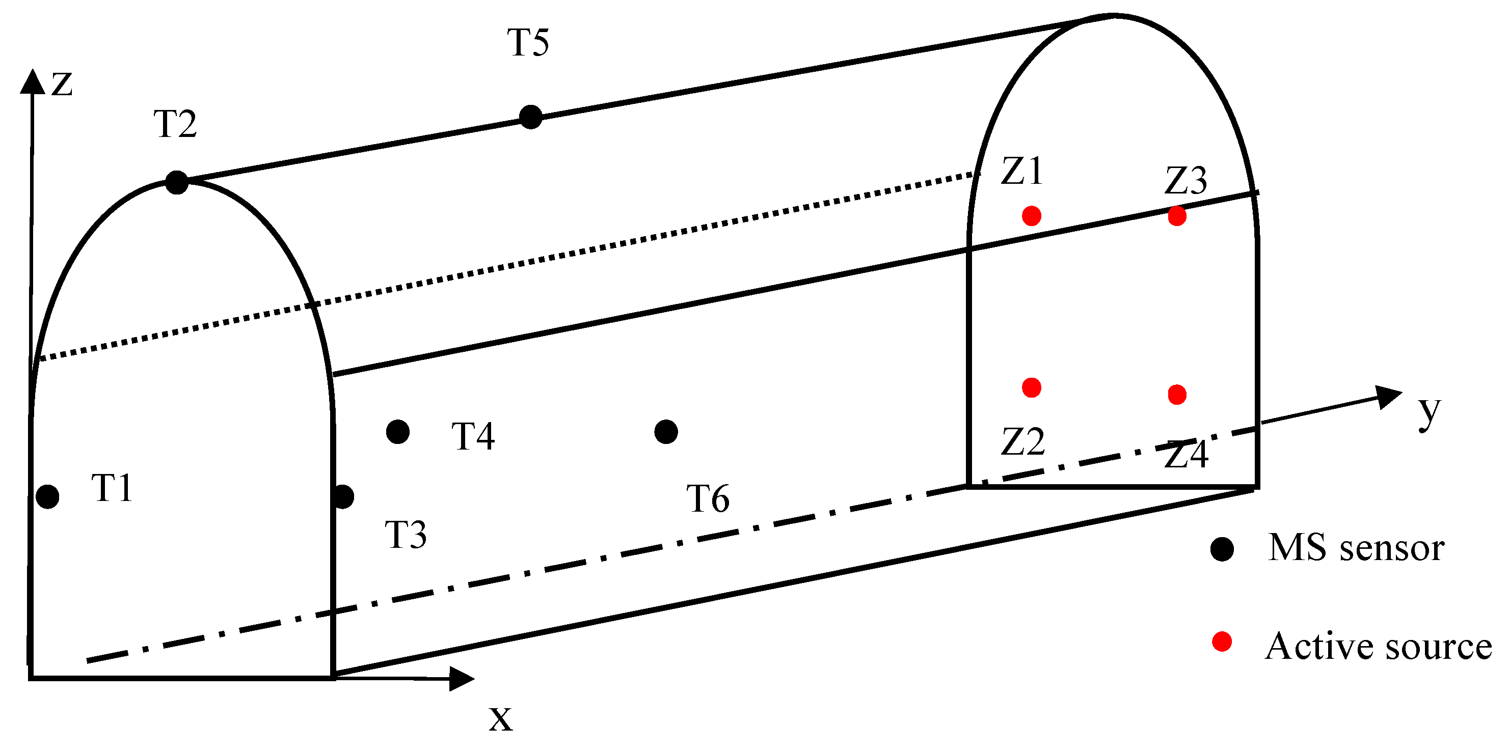
Figure 8.
For each type of velocity model, the MLKNN algorithm was used to select the velocity model, and the location error of the selected velocity model was compared with that of the best-match velocity model. The best match was the velocity model that exhibited the minimum localization error during the experiment. The white dot in the box represents the average value of location error.

Table 1.
Coordinates of the microseismic stations (MS sensors).
| Coordinates (m) | Microseismic Stations (MS Sensors) | |||||||
|---|---|---|---|---|---|---|---|---|
| 1 | 2 | 3 | 4 | 5 | 6 | 7 | 8 | |
| x | 0 | 8 | −8 | 1 | 0 | 8 | −8 | −1 |
| y | 8 | 0 | 0 | −9 | 8 | 0 | 0 | −10 |
| z | 2 | 0 | 0 | 5 | 42 | 40 | 40 | 27 |
Table 2.
Coordinates of the active sources.
| Coordinates (m) | Active Sources | ||||
|---|---|---|---|---|---|
| Z1 | Z2 | Z3 | Z4 | Z | |
| x | 2 | −4 | −3 | 3 | 0 |
| y | 3 | 2 | −4 | −3 | 0 |
| z | 102 | 102 | 102 | 102 | 102 |
Table 3.
Different velocity models.
| Type of Velocity Model | Velocity (m/s) | |||||||
|---|---|---|---|---|---|---|---|---|
| Isotropic Velocity | 4695.84 | |||||||
| Sectional Velocity Model | First Group: 4613.00 | Second Group: 4902.64 | ||||||
| Source–station velocity model-1 | 4614.91 | 4601.06 | 4601.19 | 4637.19 | 4941.81 | 4926.21 | 4926.3 | 4846.82 |
| Source–station velocity model-2 | 4614.94 | 4601.27 | 4601.02 | 4637.19 | 4941.84 | 4926.34 | 4926.19 | 4846.79 |
| Source–station velocity model-3 | 4615.15 | 4601.24 | 4601.07 | 4636.98 | 4941.94 | 4926.35 | 4926.2 | 4846.66 |
| Source–station velocity model-4 | 4615.1 | 4601.04 | 4601.24 | 4636.98 | 4941.92 | 4926.2 | 4926.32 | 4846.67 |
Table 4.
Coordinates of microseismic stations (MS sensors).
| Coordinates (m) | Microseismic Stations (MS Sensors) | |||||
|---|---|---|---|---|---|---|
| 1 | 2 | 3 | 4 | 5 | 6 | |
| x | 0.00 | 1.00 | 2.00 | 0.00 | 1.30 | 2.00 |
| y | 0.50 | 0.60 | 0.40 | 3.74 | 4.50 | 3.85 |
| z | 1.50 | 2.70 | 1.60 | 1.35 | 2.65 | 1.42 |
Table 5.
Active-source coordinates.
| Coordinates (m) | Active Source | |||
|---|---|---|---|---|
| 1 | 2 | 3 | 4 | |
| x | 0.75 | 0.75 | 1.50 | 1.50 |
| y | 8.00 | 8.00 | 8.00 | 8.00 |
| z | 1.60 | 0.40 | 1.60 | 0.40 |
Table 6.
Coordinates and travel time of MS events.
| MS Source | Coordinates (m) | Travel Time of the Events (s) | |||||||
|---|---|---|---|---|---|---|---|---|---|
| x | y | z | 1 | 2 | 3 | 4 | 5 | 6 | |
| 1 | 1.10 | 8.00 | 1.70 | 0.02450 | 0.01125 | 0.00825 | 0.00725 | 0.01700 | 0.03025 |
| 2 | 2.00 | 6.52 | 1.63 | 0.03330 | 0.00700 | 0.00400 | 0.00350 | 0.00130 | 0.00050 |
| 3 | 2.00 | 6.12 | 1.39 | 0.03100 | 0.00550 | 0.00225 | 0.00125 | 0.00200 | 0.00175 |
| 4 | 0.00 | 7.67 | 1.40 | 0.01400 | 0.02375 | 0.03625 | 0.00400 | 0.01650 | 0.02550 |
| 5 | 1.45 | 8.00 | 1.37 | 0.02575 | 0.01175 | 0.00725 | 0.01000 | 0.01550 | 0.00180 |
| 6 | 2.00 | 7.18 | 1.70 | 0.03600 | 0.00750 | 0.00425 | 0.00400 | 0.00150 | 0.00225 |
| 7 | 1.30 | 8.00 | 1.00 | 0.02125 | 0.01175 | 0.00775 | 0.00775 | 0.00500 | 0.00050 |
| 8 | 2.00 | 6.88 | 1.31 | 0.03400 | 0.00375 | 0.00350 | 0.00350 | 0.00125 | 0.00325 |
| 9 | 0.00 | 6.98 | 1.49 | 0.01400 | 0.02375 | 0.03625 | 0.00400 | 0.01650 | 0.02550 |
| 10 | 1.23 | 8.00 | 0.54 | 0.02125 | 0.01125 | 0.00775 | 0.00575 | 0.00650 | 0.00100 |
Table 7.
Different velocity models in the tunnel laboratory.
| Type of Velocity Model | Velocity (m/s) | |||||
|---|---|---|---|---|---|---|
| Isotropic velocity-1 | 387.83 | |||||
| Isotropic velocity-2 | 565.48 | |||||
| Isotropic velocity-3 | 502.25 | |||||
| Isotropic velocity-4 | 1007.23 | |||||
| Sectional velocity model-1 | First group: 500.98 | Second group: 220.51 | ||||
| Sectional velocity model-2 | First group: 995.65 | Second group: 559.37 | ||||
| Sectional velocity model-3 | First group: 516.41 | Second group: 459.92 | ||||
| Sectional velocity model-4 | First group: 1172.79 | Second group: 697.92 | ||||
| Source–station velocity model-1 | 314.09 | 564.94 | 993.82 | 525.18 | 2052.93 | 1422.26 |
| Source–station velocity model-2 | 346.24 | 674.19 | 1005.81 | 305.42 | 763.1 | 424.05 |
| Source–station velocity model-3 | 294.2 | 638.13 | 761.64 | 952.27 | 236.1 | 2091.94 |
| Source–station velocity model-4 | 255.45 | 1350.49 | 881.19 | 512.8 | 980.15 | 860.53 |
Disclaimer/Publisher’s Note: The statements, opinions and data contained in all publications are solely those of the individual author(s) and contributor(s) and not of MDPI and/or the editor(s). MDPI and/or the editor(s) disclaim responsibility for any injury to people or property resulting from any ideas, methods, instructions or products referred to in the content. |
© 2023 by the authors. Licensee MDPI, Basel, Switzerland. This article is an open access article distributed under the terms and conditions of the Creative Commons Attribution (CC BY) license (https://creativecommons.org/licenses/by/4.0/).
Share and Cite
MDPI and ACS Style
Shen, T.; Wang, S.; Jiang, X.; Peng, G.; Tuo, X. An Anisotropic Velocity Model for Microseismic Events Localization in Tunnels. Sensors 2023, 23, 4670. https://doi.org/10.3390/s23104670
AMA Style
Shen T, Wang S, Jiang X, Peng G, Tuo X. An Anisotropic Velocity Model for Microseismic Events Localization in Tunnels. Sensors. 2023; 23(10):4670. https://doi.org/10.3390/s23104670
Chicago/Turabian StyleShen, Tong, Songren Wang, Xuan Jiang, Guili Peng, and Xianguo Tuo. 2023. "An Anisotropic Velocity Model for Microseismic Events Localization in Tunnels" Sensors 23, no. 10: 4670. https://doi.org/10.3390/s23104670
Note that from the first issue of 2016, this journal uses article numbers instead of page numbers. See further details here.