
Magnetoimpedance Effect in Cobalt-Based Amorphous Ribbons with an Inhomogeneous Magnetic Structure

Department of Physics, Pedagogical Institute, Irkutsk State University, 664003 Irkutsk, Russia
*
Author to whom correspondence should be addressed.
Sensors 2023, 23(19), 8283; https://doi.org/10.3390/s23198283
Submission received: 1 September 2023
/
Revised: 29 September 2023
/
Accepted: 4 October 2023
/
Published: 7 October 2023
(This article belongs to the Special Issue Challenges and Future Trends of Magnetic Sensors)
Abstract
:The results of a computer simulation and experimental study of the magnetoimpedance effect (MI) in amorphous Co68.5Fe4.0Si15.0B12.5 and Co68.6Fe3.9Mo3.0Si12.0B12.5 ribbons in the ac frequency range from 0.01 to 100 MHz are presented. It was found that the maximum MI value exceeds 200%, which may be of interest in the development of magnetic field sensors. It is also shown that practically significant characteristics of the MI response strongly depend on the ac frequency, which is due to the inhomogeneous distribution of magnetic properties over the ribbon cross section. This distribution was studied using magnetoimpedance tomography based on the analysis of the experimental dependences of the reduced impedance on the ac frequency.
1. Introduction
The magnetoimpedance effect (MI) consists of changing the electrical impedance of a ferromagnetic conductor under the action of an external magnetic field [1]. If we confine ourselves to conductors of planar geometry, then MI is most intensively studied in amorphous magnetically soft ribbons based on cobalt and iron [2,3], including those after nanocrystallization [4,5], as well as in thin magnetic films [6,7] and multilayer films [8,9,10]. In this case, the MI is most often studied in the so-called longitudinal configuration, when the alternating current and the external magnetic field are oriented along the same axis [11].
The relative change in the impedance in the mentioned objects can reach hundreds of percents when the magnetic field intensity changes by units of A/m. For this reason, the development of highly sensitive magnetic field sensors based on MI is being actively discussed because it can be in demand both in technical [12,13,14] and biomedical applications [15,16,17].
The MI can be clearly explained in terms of the skin effect. The distribution of an alternating electric current (ac) over the cross section of a conductor with magnetic permeability μ and specific conductivity σ depends on the ac frequency f and can be characterized by the thickness of the skin layer [18]:
where μ0 is the magnetic constant.
Simplistically, it can be assumed that the alternating current is mainly concentrated in the surface layer of the conductor with a thickness equal to the thickness of the skin layer, i.e., the effective cross section of the conductor is determined by δ. Thus, it follows from expression (1) that if the magnetic permeability of the conductor changes, then its effective cross section changes. Consequently, the impedance also changes, i.e., MI is observed.
With a uniform distribution of the magnetic permeability over the cross section of a planar conductor with a thickness of 2b, its impedance, taking into account the external inductance Lext, can be represented as follows [18,19]:
where RDC is the ribbon resistance to direct current and k = (1 − j)/δ, j is an imaginary unit. External inductance is due to the magnetic flux created by the electric current outside the conductor. In the case of a rectangular conductor with length l, width a and thickness 2b, the value of Lext can be written as follows [20]:
Equation (2) shows that the contribution of an external inductance increases with an ac frequency increase. With the usual parameters for samples of cobalt-based ribbons (a = 1 mm, 2b = 25 μm and σ = 600 kS/m), the contribution of the external inductance at an ac frequency of 1 MHz is 10 times less than RDC, that at the frequency of 10 MHz becomes comparable and that at the frequency of 100 MHz exceeds RDC by 10 times. The contribution of the external inductance is often not considered when modeling MI at low ac frequencies [19]. However, at high frequencies, this contribution must be considered.
To date, theoretical concepts have been developed on how to determine the orientation of an easy magnetization axis and the magnitude of magnetic anisotropy on MI of planar magnetically soft conductors [19,21]. The frequency dispersion of the magnetic permeability and different orientations of the magnetization in neighboring magnetic domains were considered in [22]. The MI was also considered in the presence of an inhomogeneous external magnetic field [23]. The theoretical models of MI are of interest in multilayer films, the electrical and magnetic properties of which vary over the cross section [10,24]. A computer simulation using the finite element method also recommended itself in the study of MI response of such objects [8,25,26]. The effect of various coatings on the MI of amorphous magnetically soft ribbons was also studied using a computer simulation [27]. However, the influence of the nonuniform distribution of magnetic properties over the cross section of the ribbons on the MI has not been discussed either theoretically or with the help of computer simulations, although, this issue is relevant, as shown below.
Quenching stresses are irregularly distributed over the thickness of the amorphous ribbon. According to [28,29], the quenching stresses reach their maximum modulus near the surface of the ribbon, while they are minimal in its central part. Since there is no magnetocrystalline anisotropy in amorphous ribbons, the magnetoelastic anisotropy caused by quenching stresses leads to the formation of an inhomogeneous magnetic structure. It was shown when studying amorphous FePC ribbons that the distribution of the magnetic anisotropy over the thickness of the ribbon is inhomogeneous and asymmetric [30]. Its value is minimal near the middle of the ribbon and increases as it approaches the ribbon’s surfaces. This distribution of the magnetic anisotropy correlates with the quenching stress distribution over the ribbons’ cross sections described above.
Another factor affecting the distribution of magnetic properties over the cross section of the ribbon is surface irregularities [29,31,32]. The effect of irregularities on the magnetic anisotropy parameters of an amorphous ribbon is especially strong in the case of zero magnetostriction [32]. Surface irregularities can also cause an increase in the magnetic anisotropy dispersion [31,33], which can strongly affect the MI, especially at high frequencies [34]. Polishing and other modifications of the ribbon surface lead to a significant change in the MI response [35,36].
If the magnetic parameters are not uniformly distributed over the ribbon cross section, then different regions of the ribbon, which may have different magnetic anisotropy parameters, are involved in the formation of the MI response at different ac frequencies due to different skin layer thicknesses. In this case, it is fair to expect that the nature of the MI response depends on the ac frequency. This is also supported by numerous experimental results, for example [37]. Thus, the inhomogeneity of the ribbon magnetic structure must be considered when developing MI sensors. Knowing the distribution of the magnetic properties over the ribbon cross section and how it changes depending on the choice of manufacturing conditions and further heat treatment, it is possible to purposefully tune the characteristics of MI sensors based on amorphous ribbons for a specific task.
To establish the distribution of the magnetic properties over the cross section of amorphous and electrodeposited wires, a method called magnetic impedance tomography (MIT) was proposed [38]. This method is based on the analysis of the impedance dependences on the ac frequency. In this paper, we propose an implementation of this method for amorphous ribbons.
2. Samples, Experimental Methods and Computer Simulation
2.1. Description of the Samples
The ribbons Co68.5Fe4.0Si15.0B12.5 (S0) and Co68.6Fe3.9Mo3.0Si12.0B12.5 (S1) were prepared by rapid quenching using the Cu weal technique. The nominal widths of the S0 and S1 ribbons were 0.71 mm and 0.78 mm, respectively. The thicknesses of the S0 and S1 ribbons were 24 and 26 μm, respectively. Samples 30 mm long were cut from the original ribbon. Designations of the samples, their geometrical parameters, values of magnetostriction and specific conductivity are given in Table 1.
2.2. Experimental Methods
The modulus of the electrical impedance Z was measured using the measuring complex of magnetoimpedance spectroscopy. A measuring setup was developed by the authors of this article. A photograph of the setup is shown in Figure 1; its detailed description is given in [11]. The distance between the contacts of the measuring cell was l = 24 mm. The effective value of the alternating current was equal to 1 mA. The alternating current frequency, f, varied in the range 0.01–80 MHz. An external magnetic field, H, was generated by a pair of Helmholtz coils. Its maximum strength was Hmax = ±12.3 kA/m. The alternating current and the external magnetic field were oriented along the length of the sample.
MI was calculated using the following formula:
The magnetic hysteresis loops were obtained using the induction method. The remagnetizing magnetic field oriented along the length of the sample varied with a frequency of 1 kHz, and its amplitude was 1.2 kA/m.
Saturation magnetostriction, λS, was determined using the approach of changing the peak field in the ΔZ/Z(H) dependence under the action of tensile mechanical stresses γ. This approach was proposed in [39]. The maximum values of the mechanical stresses, γmax, were 575 MPa and 480 MPa for the S0 and S1 ribbons, respectively.
2.3. Computer Simulation of the MI
A computer simulation of the MI was performed using the finite element method in Comsol Multiphysics software in the ac frequency range from 0.01 to 80 MHz (license no. 9602434). The ribbon model had a rectangular section 2b × a and length l. The section of the model was divided into a stack of 2n − 1 layers of a rectangular section, arranged symmetrically with respect to its middle (Figure 2b). The width and length of each layer were a and l, respectively. For each layer, the value of the transverse magnetic permeability μi was set according to the following system of equations:
where yi is the coordinate of the outer boundary of the i-th layer. Obviously, |yn| = b. The specific conductivities of the layers were assumed to be the same and equal to σ (see Table 1). Models with n from 1 to 6 were considered.
To simulate the magnetic flux outside the ribbon in Comsol Multiphysics, the circular section Air with radius 2a was used (Figure 3). The magnetic permeability of this region is 1, the permittivity is 1 and the specific conductivity is 0. The closing of the magnetic field lines at infinity was considered using the Infinite Element Domain tool (outer cylindrical layers of the model in Figure 3). It should be noted that, we made sure that the size of finite element mesh elements was less than the thickness of the skin layer. Figure 3c also shows an example of calculating the distribution of magnetic induction in and around the ribbon.
2.4. Implementation of Magnetic Impedance Tomography of Amorphous Ribbons
MIT was used in this work to estimate the distribution of magnetic permeability over the amorphous ribbons’ cross sections. This method was implemented as described below.
- The distribution of the magnetic permeability was set according to the system of Equation (5) and Table 2. In this case, μi varied from 1 to 25,000.
- Using solutions for the electric and magnetic field obtained with Comsol Multiphysics for various combinations of μi values, the dependences of the reduced impedance on the ac frequency Z(f)/RDC were calculated.
- In the array of the simulated Z(f)/RDC dependences, we found the one that had the smallest absolute deviation from the Z(f)/RDC dependence obtained experimentally.
- The combination of μi values at which the simulated dependence Z(f)/RDC has the smallest deviation from the experimental one is, presumably, an approximation of the actual distribution of the magnetic permeability over the ribbon cross section.
The dependence of the magnetic permeability on the ac frequency can be described using the Landau–Lifshitz–Gilbert equation (see for example [40]). The greater the Gilbert damping parameter kG included in this equation, the more the magnetic permeability changes with frequency. For amorphous CoFeSiB alloys, the typical kG value is around 0.03 [41]. With this parameter value, the magnetic permeability module at the frequency of 80 MHz differs from the magnetic permeability module at the frequency of 0.01 MHz by several percent. Therefore, to simplify the modeling in this work, we neglect the frequency dependence of the magnetic permeability modulus. However, it should be noted that the real and especially imaginary component of the magnetic permeability changes with the ac frequency much more significantly than the modulus. Therefore, taking into account magnetic permeability dependence on the ac frequency is strictly necessary when determining its components using MIT. Obviously, for this, it will be necessary to analyze not the impedance modulus, but the resistance and reactance. The determination of the magnetic permeability components using MIT will be discussed in further articles devoted to the development of this method.
3. Results and Discussion
3.1. Experimental Results
The saturation magnetization of both ribbons is about MS ≈ 560 kA/m (Figure 4). The coercive force in both cases is about 50 A/m. Thus, according to the magnetic hysteresis loops, the ribbons have pronounced soft magnetic properties.
The saturation magnetostriction, determined as described in Section 2.2, is –0.18⋯10−7 and +0.59⋯10−7 for samples S0 and S1, respectively. It should be noted that the obtained magnetostriction values are in good agreement with the results obtained for similar ribbons based on the analysis of changes in hysteresis loops under the action of tensile mechanical stresses [42].
The value of (ΔZ/Z)max corresponds to the peak in the magnetic field dependence of the MI and reaches its maximum value at an ac frequency of about 8 MHz in the case of S1 ribbons (Figure 5). In this case, (ΔZ/Z)max exceeds 200%, which may be of practical interest.
In the case of the S0 ribbons, the dependence (ΔZ/Z)max(f) has the same characteristics as in the case of S1 ribbons (Figure 5). However, the highest MI value in these ribbons exceeds 250%, which is observed at an ac frequency of about 8 MHz.
Both in the case of the S1 ribbons and of the S0 ribbons, the MI dependences on the external magnetic field strength ΔZ/Z(H) in the entire ac frequency range have two peaks. This is expressed as the stronger the ΔZ/Z(H), the higher the f. In addition, an increase in the magnetic field strength Hp is observed with an increase in the frequency of the alternating current. For S1 ribbons, the minimum value of the peak field is Hp1 ≈ 60 A/m and the maximum value is Hp2 ≈ 320 A/m (Figure 6b). In turn, for S0 ribbons, these values are approximately 20 and 260 A/m, respectively (Figure 6a). The described changes in Hp with ac frequency increasing, as well as an increase in the increasing portion of the ΔZ/Z(H) dependence may be associated with the inhomogeneous distribution of the magnetic permeability over the cross section of the S0 and S1 ribbons [38].
3.2. MIT Results
Details of the magnetic permeability distribution over the ribbon cross section were restored using MIT (see Section 2.4) based on the analysis of the experimental Z(f)/RDC dependences (Figure 7 and Figure 8, solid lines). These dependencies consist of two sections: an almost horizontal section Z/RDC ≈ 1, which at a certain alternating current frequency f0, smoothly transforms into an increasing section. It should be noted that there are features such as kinks and changes in the angle of inclination in low magnetic fields in the increasing section of the Z(f)/RDC dependence. It may indicate a non-uniform distribution of the magnetic permeability over the cross section of the ribbon [38]. In magnetic fields close to Hmax, the increasing section is almost a straight line, indicating a distribution of magnetic permeability that is close to uniform.
The Z(f)/RDC dependences reconstructed from the MIT results at n = 1 (uniform distribution of the magnetic permeability over the ribbon cross section) differ significantly from the experimental ones obtained in low magnetic fields (Figure 7a and Figure 8a, markers). The relative deviation for some ac frequencies exceeds 80% and confirms the conclusion about the inhomogeneous magnetic structure of the ribbons. An increase in n in the model leads to a decrease in the deviation of the reconstructed Z(f)/RDC dependences from the experimental ones. Thus, at n = 3, the Z(f)/RDC dependences reconstructed using MIT deviate from the experimental ones by no more than 6%. Increasing the number of layers to six made it possible to ensure that the deviation did not exceed 3% over the entire studied range of the magnetic fields.
At the same time, at Hmax, the Z(f)/RDC dependences, constructed from the MIT results, even at n = 1, deviate from the experimental ones by no more than 3% (Figure 7b and Figure 8b markers). This confirms the conclusion that with external magnetic field strength increasing, the distribution of the magnetic permeability over the ribbons cross section becomes more uniform. When using the model with n = 6, the deviation of the reconstructed and experimental dependencies does not exceed 1%.
It should also be noted that the deviation of the simulated and experimental dependences may be due to the fact that the frequency dispersion of the magnetic permeability, including the dispersion of the magnetic permeability associated with the motion of domain walls, is not taken into account. Moreover, symmetrical models were used for MIT, while the distribution of magnetic permeability can be asymmetric due to the asymmetric distribution of hardening stresses and the different state of the contact and free surfaces of the ribbon [28,29,30,31,32,33].
Magnetic permeability distributions reconstructed using MIT for n = 6 are shown in Figure 9 for the S0 ribbon and in Figure 10 for the S1 ribbon.
According to the MIT results, the permeability of the S0 ribbon surface layer that is 1 µm thick is about 140 in the absence of the external magnetic field (Figure 9). The permeability of the next layer is much higher—more than 4000. With further advancement in depth, the magnetic permeability gradually increases, reaching 17,000 in the central part of the ribbon.
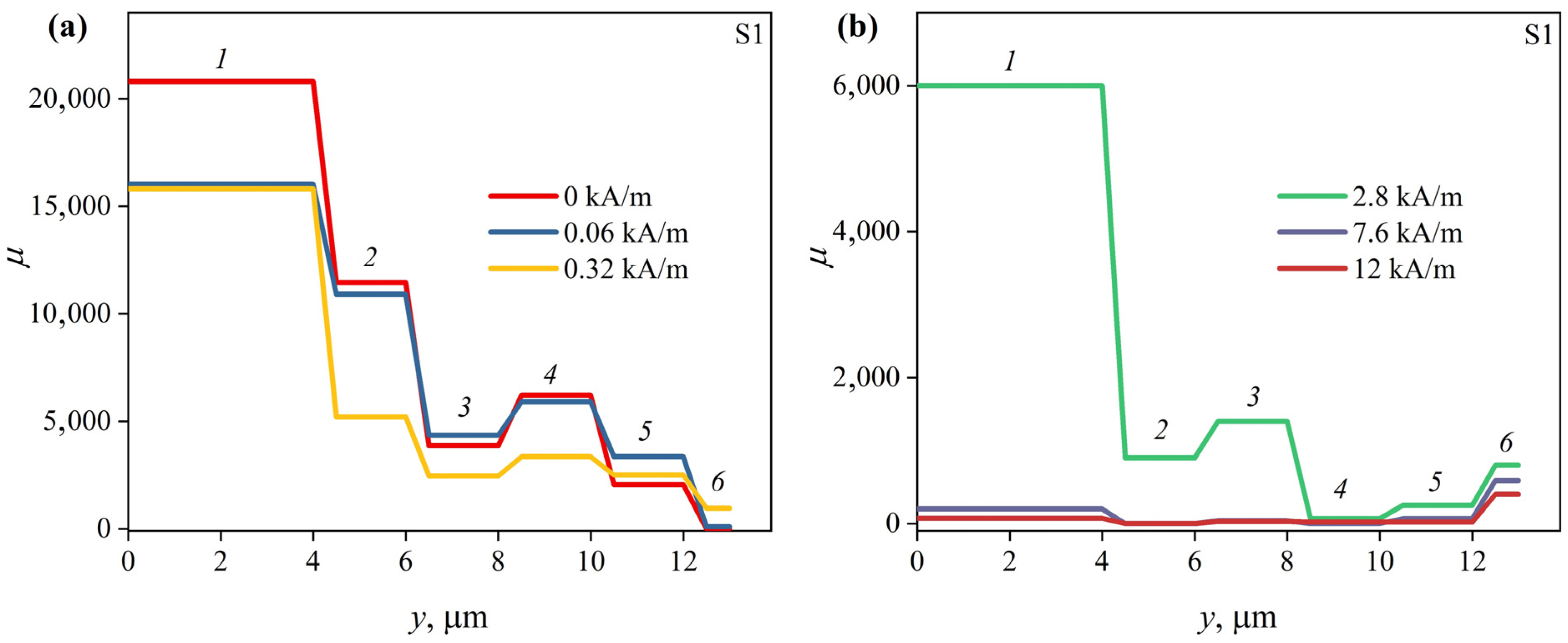
The permeability of the surface layer of the S1 ribbon is also low—about 10 (Figure 10). However, the details of the magnetic permeability distribution in the inner regions of the S1 ribbon are somewhat different from those of the S0 ribbon. Thus, at H = 0, the magnetic permeability first increases from 2000 to 6200, then decreases to 3800 and then increases again when moving deep into the ribbon from layer 5 to layer 2 (see Table 2). The magnetic permeability of the central layer exceeds 20,000. Note that internal quenching stresses at some distance from the ribbon surface can change their sign, passing through 0 [28,29]. In this region, the magnetoelastic energy 3λsγin/2 (γin is the internal quenching stress) can also be near zero. This, apparently, determines the higher magnetic permeability in layer 4 compared to that in neighboring layers.
Next, consider how the magnetic permeability changes with a change in the external magnetic field.
As H increases, the magnetic permeability of the outer layer of the S0 ribbon first increases, reaching a maximum value of about 950 at H = Hp2, and then decreases. It reaches 300 at Hmax (Figure 9). The magnetic permeabilities of layers 4–5, as well as the permeability of layer 2, reach their maximum values in lower fields, at H = Hp1. The magnetic permeabilities of the remaining layers decrease with increasing external magnetic field strength. Note that the inner layers, in contrast to the surface ones, are close to saturation at Hmax. Their magnetic permeabilities are about 1.
In the case of ribbon S1, an increase in the magnetic field strength from 0 to Hp1 leads to an increase in the magnetic permeability of layers 3, 5 and 6. The permeability of layer 4 practically does not change in this case. The magnetic permeability of layer 5 increases most noticeably. The magnetic permeability, as in the case of S0 ribbons, decreases in the entire ribbon with the subsequent increase in H, except for the surface layer. Its permeability continues to increase, reaching a value of about 950 and then decreasing to about 400 at Hmax.
Probably, the increase in the MI at low frequencies is mainly due to an increase in the magnetic permeability of the inner regions of the ribbon both in the case of the S1 ribbon and in the case of the S0 ribbon. The nature of the ΔZ/Z(H) dependence at high frequencies is mainly determined by the magnetic field dependence of the magnetic permeability surface layer.
The peculiarities of the change in the magnetic permeability of the surface layers of both ribbons indicates a predominantly transverse orientation of the EMA in them. At the same time, the maximum values of these permeabilities are small. This is probably due to the significant anisotropy dispersion caused by non-uniform relief of the ribbon. Also, the magnetic permeabilities of the surface layers of the ribbons are far from saturation, even at Hmax, due to the anisotropy dispersion. This, along with the high contribution of the external inductance 2πfLext (see expression (2)) limits the maximum MI at high ac frequencies (Figure 5), which must be taken into account when developing MI sensors.
The magnetic anisotropy of the ribbon inner regions is predominantly longitudinal. This is indicated by high values of the magnetic permeability and its decrease with increasing H. An increase in the permeability of some inner layers with a change in the magnetic field from 0 to Hp1 is presumably associated with a decrease in the magnetic anisotropy dispersion. Based on this, it can be assumed that quenching stresses do not have a decisive effect on the orientation of the EMA. Otherwise, the orientation of the EMA in the inner and outer regions of the S0 and S1 ribbons would be different since the signs of their magnetostriction constants are different. It is likely that the EMA orientation is strongly affected by the anisotropy of the ribbons’ shape. However, the energy of magnetoelastic anisotropy can affect the values of magnetic permeability due to the quenching stresses. The magnetoelastic energy 3λsγin/2 of the S0 ribbon is smaller, since its magnetostriction is smaller in modulus. This leads to the fact that the magnetic permeability of the inner region of the S0 ribbon is higher than that of the S1 ribbon. According to the literature [28,29], the quenching stresses in the central part are very low, which seems to be responsible for the high magnetic permeability of both ribbons.
The practical significance of MIT deserves special attention. As is known, amorphous soft magnetic ribbons obtained by rapid quenching from a melt are characterized by a noticeable scatter of functional characteristics even within the same batch. Despite this, a minimum scatter of metrological characteristics must be ensured when manufacturing devices using these materials, especially MI magnetic field sensors. This can be achieved by selecting pieces of ribbons with similar distributions of magnetic characteristics using MIT. In addition, MIT may be in demand when monitoring changes in the magnetic structure during heat treatment, which is often used to improve the functional properties of amorphous ribbons [43,44].
4. Conclusions
Thus, based on the analysis of the experimental ΔZ/Z(H) and Z(f)/RDC dependences, it was shown that Co68.5Fe4.0Si15.0B12.5 (S0) amorphous ribbons with magnetostriction λs ≈ –0.18 · 10−7 and Co68.6Fe3.9Mo3.0Si12.0B12.5 (S1) with magnetostriction λs ≈ +0.59 · 10−7 have an inhomogeneous magnetic structure. Details of the distribution of magnetic permeability over the ribbons’ cross section were reconstructed using MIT based on an analysis of the experimental Z(f)/RDC dependences obtained in the ac frequency range from 0.01 to 80 MHz in magnetic fields of various strengths.
According to the MIT, the magnetic permeability distribution over the cross section of both ribbons is nonuniform. The surface layers of both ribbons have predominantly transverse magnetic anisotropy. In this case, the low values of their magnetic permeability indicate a significant dispersion of the magnetic anisotropy associated with the surface topography. The magnetic permeability of the inner layers of both ribbons is much higher than that of the surface ones, and the nature of its change in the magnetic field indicates that the magnetic anisotropy of the inner layers is predominantly longitudinal.
The influence of magnetostriction is manifested in the fact that the magnetic permeability of the inner layers of the Co68.5Fe4Si15.0B12.5 ribbon is generally higher than that of the Co68.6Fe3.9Mo3.0Si12.0B12.5 ribbon, since its magnetostriction is lower in the modulus, respectively, and the magnetoelastic energy associated with quenching stresses is less.
The distribution of the magnetic properties over the cross section of amorphous magnetically soft ribbons, reconstructed using MIT, must be taken into account when choosing the optimal operating modes for MI sensors. It should also be noted that the MIT can be in demand in the manufacture of devices based on amorphous ribbons to ensure the minimum spread of their characteristics.
Author Contributions
Conceptualization, D.A.B.; Investigation, M.S.D.; Methodology, D.A.B., M.S.D. and A.V.S.; Project administration, D.A.B.; Software, M.S.D.; Supervision, D.A.B.; Validation, D.A.B., M.S.D. and A.V.S.; Visualization, M.S.D.; Writing—original draft, D.A.B. and M.S.D.; Writing—review and editing, A.V.S. All authors have read and agreed to the published version of the manuscript.
Funding
The modeling and measurements of the impedance were carried out at Irkutsk State University and supported by the Russian Science Foundation (grant no. 22-22-00709, https://rscf.ru/project/22-22-00709/ (accessed on 5 October 2023).
Institutional Review Board Statement
Not applicable.
Informed Consent Statement
Not applicable.
Data Availability Statement
The data are available from the corresponding author upon reasonable request.
Conflicts of Interest
The authors declare no conflict of interest.
References
- Beach, R.S.; Berkowitz, A.E. Sensitive field- and frequency-dependent impedance spectra of amorphous FeCoSiB wire and ribbon (invited). J. Appl. Phys. 1994, 76, 6209–6213. [Google Scholar] [CrossRef]
- Kurlyandskaya, G.V.; Lezama, L.; Pasynkova, A.A.; Volchkov, S.O.; Lukshina, V.A.; Larrañaga, A.; Dmitrieva, N.V.; Timofeeva, A.V.; Orue, I. Amorphous FeCoCrSiB Ribbons with Tailored Anisotropy for the Development of Magnetic Elements for High Frequency Applications. Materials 2022, 15, 4160. [Google Scholar] [CrossRef] [PubMed]
- Arzuza, L.C.C.; Béron, F.; Pirota, K.R. High-frequency GMI hysteresis effect analysis by first-order reversal curve (FORC) method. J. Magn. Magn. Mater. 2021, 534, 168008. [Google Scholar] [CrossRef]
- Tejedor, M.; Hernando, B.; Sánchez, M.; Prida, V.; Garcia-Beneytez, J.; Vázquez, M.; Herzer, G. Magnetoimpedance effect in zero magnetostriction nanocrystalline Fe73.5Cu1Nb3Si16.5B6 ribbons. J. Magn. Magn. Mater. 1998, 185, 61–65. [Google Scholar] [CrossRef]
- Dwevedi, S.; Markandeyulu, G.; Ohodnicki, P.R.; Leary, A.; McHenry, M.E. Stress-MI and domain studies in Co-based nanocrystalline ribbons. J. Magn. Magn. Mater. 2011, 323, 1929–1933. [Google Scholar] [CrossRef]
- Kikuchi, H.; Kamata, S.; Takahashi, Y.; Nakai, T.; Hashi, S.; Ishiyama, K. Investigation of driving power dependence on magnetoimpedance properties of thin-film elements with uniaxial anisotropy. IEEE Trans. Magn. 2015, 51. [Google Scholar] [CrossRef]
- Garcίa, D.; Muñoz, J.; Kurlyandskaya, G.; Vázquez, M.; Ali, M.; Gibbs, M.R. Induced anisotropy, magnetic domain structure and magnetoimpedance effect in CoFeB amorphous thin films. J. Magn. Magn. Mater. 1999, 191, 339–344. [Google Scholar] [CrossRef]
- García-Arribas, A.; Fernández, E.; Svalov, A.; Kurlyandskaya, G.V.; Barandiaran, J.M. Thin-film magneto-impedance structures with very large sensitivity. J. Magn. Magn. Mater. 2016, 400, 321–326. [Google Scholar] [CrossRef]
- Chen, J.-A.; Ding, W.; Zhou, Y.; Cao, Y.; Zhou, Z.-M.; Zhang, Y.-M. Stress-impedance effects in sandwiched FeCuNbCrSiB/Cu/FeCuNbCrSiB films. Mater. Lett. 2006, 60, 2554–2557. [Google Scholar] [CrossRef]
- Antonov, A.S.; Gadetskii, S.N.; Granovskii, A.B.; D’yachkov, A.L.; Paramonov, V.P.; Perov, N.S.; Prokoshin, A.F.; Usov, N.A.; Lagar’kov, A.N. Giant magnetoimpedance in amorphous and nanocrystalline multilayers. Phys. Met. Metallogr. 1997, 83, 612–618. [Google Scholar]
- Bukreev, D.A.; Derevyanko, M.S.; Moiseev, A.A.; Semirov, A.V.; Savin, P.A.; Kurlyandskaya, G.V. Magnetoimpedance and Stress-Impedance Effects in Amorphous CoFeSiB Ribbons at Elevated Temperatures. Materials 2020, 13, 3216. [Google Scholar] [CrossRef] [PubMed]
- Zhan, Z.; Yaoming, L.; Jin, C.; Yunfeng, X. Current sensor utilizing giant magneto-impedance effect in amorphous ribbon toroidal core and CMOS inverter multivibrator. Sens. Actuators A Phys. 2007, 137, 64–67. [Google Scholar] [CrossRef]
- Gazda, P.; Szewczyk, R. Novel Giant Magnetoimpedance Magnetic Field Sensor. Sensors 2020, 20, 691. [Google Scholar] [CrossRef] [PubMed]
- Feng, Z.; Zhi, S.; Wei, M.; Zhou, Y.; Liu, C.; Lei, C. An integrated three-dimensional micro-solenoid giant magnetoimpedance sensing system based on MEMS technology. Sens. Actuators A Phys. 2019, 299, 111640. [Google Scholar] [CrossRef]
- Kurlyandskaya, G.V.; Sánchez, M.L.; Hernando, B.; Prida, V.M.; Gorria, P.; Tejedor, M. Giant-magnetoimpedance-based sensitive element as a model for biosensors. Appl. Phys. Lett. 2003, 82, 3053–3055. [Google Scholar] [CrossRef]
- Yang, H.; Chen, L.; Lei, C.; Zhang, J.; Li, D.; Zhou, Z.-M.; Bao, C.-C.; Hu, H.-Y.; Chen, X.; Cui, F.; et al. Giant magnetoimpedance-based microchannel system for quick and parallel genotyping of human papilloma virus type 16/18. Appl. Phys. Lett. 2010, 97, 043702. [Google Scholar] [CrossRef]
- Yang, Z.; Wang, H.; Dong, X.; Yan, H.; Lei, C.; Luo, Y. Giant magnetoimpedance based immunoassay for cardiac biomarker myoglobin. Anal. Methods 2017, 9, 3636–3642. [Google Scholar] [CrossRef]
- Landau, L.D.; Lifshitz, E.M. Electrodynamics of Continuous Media; Pergamon Press: Oxford, UK, 1960. [Google Scholar]
- Kraus, L. Theory of giant magneto-impedance in the planar conductor with uniaxial magnetic anisotropy. J. Magn. Magn. Mater. 1999, 195, 764–778. [Google Scholar] [CrossRef]
- Kalantarov, P.L.; Tseytlin, L.A. Raschet Induktivnostey [Calculation of inductances], 3rd ed.; Energoatomizdat, Leningrad; 1986; 488 p., (Rus). [Google Scholar]
- Pirota, K.R.; Kraus, L.; Knobel, M.; Pagliuso, P.G.; Rettori, C. Angular dependence of giant magnetoimpedance in an amorphous Co-Fe-Si-B ribbon. Phys. Rev. B. 1999, 60, 6685–6691. [Google Scholar] [CrossRef]
- Dong, C.; Chen, S.; Hsu, T.Y. A modified model of GMI effect in amorphous films with transverse magnetic anisotropy. J. Magn. Magn. Mater. 2003, 263, 78–82. [Google Scholar] [CrossRef]
- Rouhani, A.A.; Matin, L.F.; Mohseni, S.M.; Zoriasatain, S. A Domain Dynamic Model Study of Magneto-impedance Sensor in the Presence of Inhomogeneous Magnetic Fields. J. Supercond. Nov. Magn. 2021, 34, 571–580. [Google Scholar] [CrossRef]
- Buznikov, N.A.; Kurlyandskaya, G.V. Magnetoimpedance in Symmetric and Non-Symmetric Nanostructured Multilayers: A Theoretical Study. Sensors 2019, 19, 1761. [Google Scholar] [CrossRef] [PubMed]
- García-Arribas, A.; Barandiarán, J.M.; de Cos, D. Finite element method calculations of GMI in thin films and sandwiched structures: Size and edge effects. J. Magn. Magn. Mater. 2008, 320, e4–e7. [Google Scholar] [CrossRef]
- Li, B.; Kosel, J. Three dimensional simulation of giant magneto-impedance effect in thin film structures. J. Appl. Phys. 2011, 109, 07E519. [Google Scholar] [CrossRef]
- Volchkov, S.O.; Pasynkova, A.A.; Derevyanko, M.S.; Bukreev, D.A.; Kozlov, N.V.; Svalov, A.V.; Semirov, A.V. Magnetoimpedance of CoFeCrSiB Ribbon-Based Sensitive Element with FeNi Covering: Experiment and Modeling. Sensors 2021, 21, 6728. [Google Scholar] [CrossRef]
- Bengus, V.Z.; Duhaj, P.; Korolkova, E.B.; Ocelík, V. Internal Stress Contribution to the Yield Stress Anisotropy of Amorphous Alloy Ribbons. Solid State Phenom. 1993, 35–36, 575–580. [Google Scholar] [CrossRef]
- Tejedor, M.; Garcı, J.A.; Carrizo, J.; Elbaile, L.; Santos, J.D. Effect of residual stresses and surface roughness on coercive force in amorphous alloys. J. Appl. Phys. 2002, 91, 8435. [Google Scholar] [CrossRef]
- Takahashi, M.; Miyazaki, T. Magnetic Anisotropy in an Amorphous Fe80P13C7 Alloy. Jpn. J. Appl. Phys. 1979, 18, 743–752. [Google Scholar] [CrossRef]
- Tsukahara, S.; Satoh, T.; Tsushima, T. Magnetic anisotropy distribution near the surface of amorphous ribbons. IEEE Trans. Magn. 1978, 14, 1022–1024. [Google Scholar] [CrossRef]
- Kraus, L.; Tomáš, I.; Keatociivílová, E.; Speingmann, B.; Müller, K. Magnetic anisotropy caused by oriented surface roughness of amorphous ribbons. Phys. Status Solidi. 1987, 100, 289–299. [Google Scholar] [CrossRef]
- Vavassori, P.; Callegaro, L.; Puppin, E.; Malizia, F.; Ronconi, F. Surface magnetic characterization of FeB amorphous ribbons. J. Magn. Magn. Mater. 1996, 157–158, 171–172. [Google Scholar] [CrossRef]
- Semirov, A.V.; Bukreev, D.A.; Moiseev, A.A.; Derevyanko, M.S.; Kudryavtsev, V.O. Relationship Between the Temperature Changes of the Magnetostriction Constant and the Impedance of Amorphous Elastically Deformed Soft Magnetic Cobalt-Based Ribbons. Russ. Phys. J. 2013, 55, 977–982. [Google Scholar] [CrossRef]
- Amalou, F.; Gijs, M.A.M. Giant magnetoimpedance of chemically thinned and polished magnetic amorphous ribbons. J. Appl. Phys. 2001, 90, 3466–3470. [Google Scholar] [CrossRef]
- Lotfollahi, Z.; Amirabadizadeh, A.; Safronov, A.P.; Beketov, I.V.; Kurlyandskaya, G.V. Magnetoimpedance Effect in CoFeMoSiB As-Quenched and Surface Modified Amorphous Ribbons in the Presence of Igon Oxide Nanoparticles of Water-Based Ferrofluid. J. Sensors. 2017, 2017, 1–9. [Google Scholar] [CrossRef]
- Yang, Z.; Chlenova, A.A.; Golubeva, E.V.; Volchkov, S.O.; Guo, P.; Shcherbinin, S.V.; Kurlyandskaya, G.V. Magnetoimpedance Effect in the Ribbon-Based Patterned Soft Ferromagnetic Meander-Shaped Elements for Sensor Application. Sensors 2019, 19, 2468. [Google Scholar] [CrossRef]
- Bukreev, D.A.; Derevyanko, M.S.; Moiseev, A.A.; Svalov, A.V.; Semirov, A.V. The Study of the Distribution of Electrical and Magnetic Properties over the Conductor Cross-Section Using Magnetoimpedance Tomography: Modeling and Experiment. Sensors 2022, 22, 9512. [Google Scholar] [CrossRef]
- Knobel, M.; Gómez-Polo, C.; Vázquez, M. Evaluation of the linear magnetostriction in amorphous wires using the giant magneto-impedance effect. J. Magn. Magn. Mater. 1996, 160, 243–244. [Google Scholar] [CrossRef]
- Usov, N.A.; Antonov, A.S.; Lagar’kov, A.N. Theory of giant magneto-impedance effect in amorphous wires with different types of magnetic anisotropy, J. Magn. Magn. Mater. 1998, 185, 159–173. [Google Scholar] [CrossRef]
- Ménard, D.; Britel, M.; Ciureanu, P.; Yelon, A. Giant magnetoimpedance in a cylindrical magnetic conductor. J. Appl. Phys. 1998, 84, 2805–2814. [Google Scholar] [CrossRef]
- Lotfollahi, Z.; García-Arribas, A.; Amirabadizadeh, A.; Orue, I.; Kurlyandskaya, G.V. Comparative study of magnetic and magnetoimpedance properties of CoFeSiB-based amorphous ribbons of the same geometry with Mo or W additions. J. Alloys Compd. 2017, 693, 767–776. [Google Scholar] [CrossRef]
- Liu, J.; Du, Z.; Jiang, S.; Shen, H.; Li, Z.; Xing, D.; Ma, W.; Sun, J. Tailoring giant magnetoimpedance effect of Co-based microwires for optimum efficiency by self-designed square-wave pulse current annealing. J. Magn. Magn. Mater. 2015, 385, 145–150. [Google Scholar] [CrossRef]
- Tehranchi, M.M.; Ghanaatshoar, M.; Mohseni, S.M.; Coisson, M.; Vázquez, M. Temperature dependence of magnetoimpedance in annealed Co-based ribbons. J. Non. Cryst. Solids. 2005, 351, 2983–2986. [Google Scholar] [CrossRef]
Figure 1.
Photograph of the measuring setup. 1—Agilent 4294A impedance analyzer (Keysight Technologies, Santa Rosa, CA, USA); 2—Agilent N6700B (Keysight Technologies, Santa Rosa, CA, USA) power supply for Helmholtz coils; 3—Helmholtz coils; 4—pipe-holder of the measuring cell, which can also be used as part of a heating system (more details in [11]); 5—measuring cell; 6—three pairs of Helmholtz coils to compensate for geomagnetic and effective laboratory fields (coils’ power supplies are not shown).

Figure 2.
Schematic representation of the ribbon (a) and splitting the ribbon model into layers (b).
Figure 2.
Schematic representation of the ribbon (a) and splitting the ribbon model into layers (b).
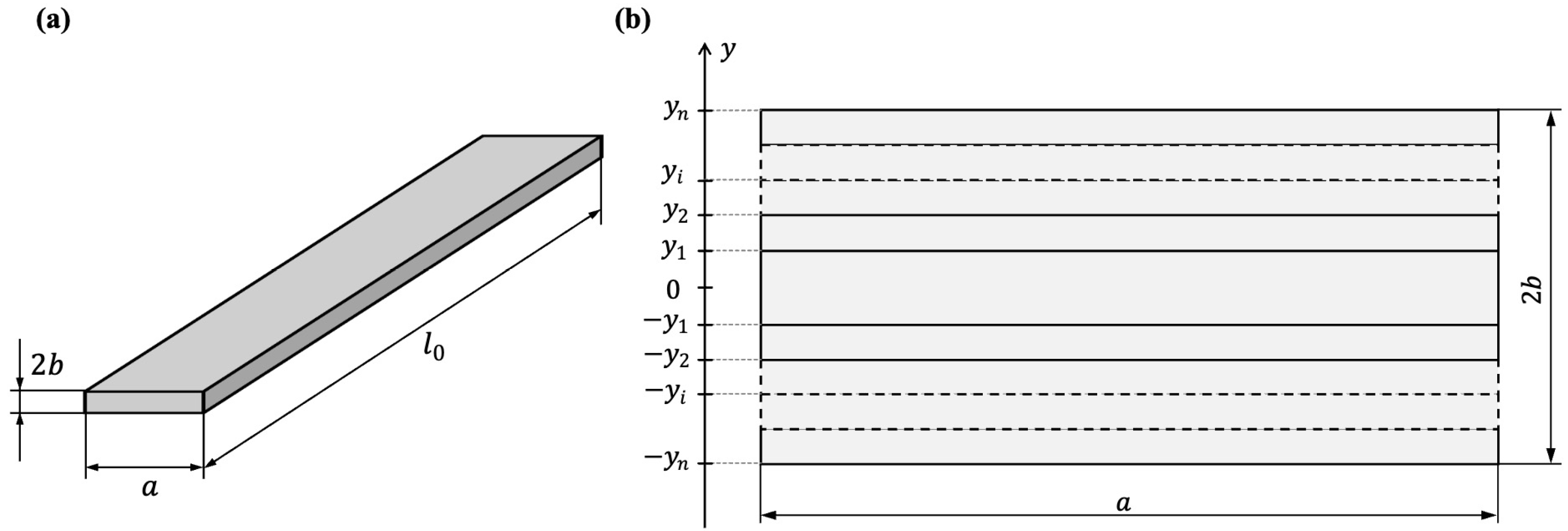
Figure 3.
A model for calculating the MI response of the ribbon with the finite element method using Comsol Multiphysics (a), fragmentation into a finite element mesh (b) and the result of calculating the magnetic induction in the ribbon and the surrounding space (c).
Figure 3.
A model for calculating the MI response of the ribbon with the finite element method using Comsol Multiphysics (a), fragmentation into a finite element mesh (b) and the result of calculating the magnetic induction in the ribbon and the surrounding space (c).

Figure 4.
Magnetic hysteresis loops of S0 and S1 ribbons.

Figure 5.
Frequency dependences of the highest MI value (ΔZ/Z)max(f) in S0 and S1 ribbons.
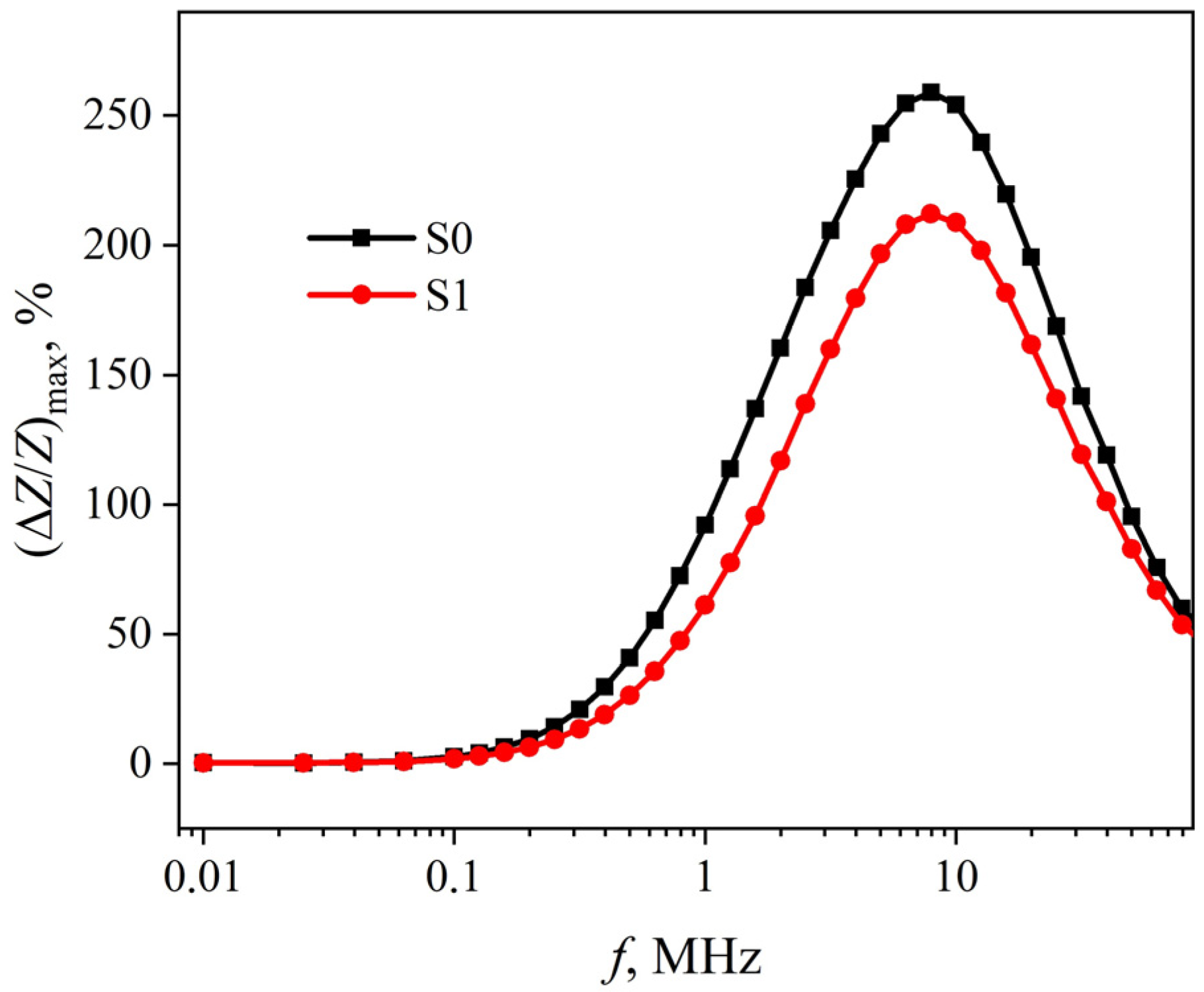
Figure 6.
Dependences of the magnetoimpedance effect in the S0 (a) and S1 (b) ribbons on the external magnetic field strength, obtained at various ac frequencies.
Figure 6.
Dependences of the magnetoimpedance effect in the S0 (a) and S1 (b) ribbons on the external magnetic field strength, obtained at various ac frequencies.
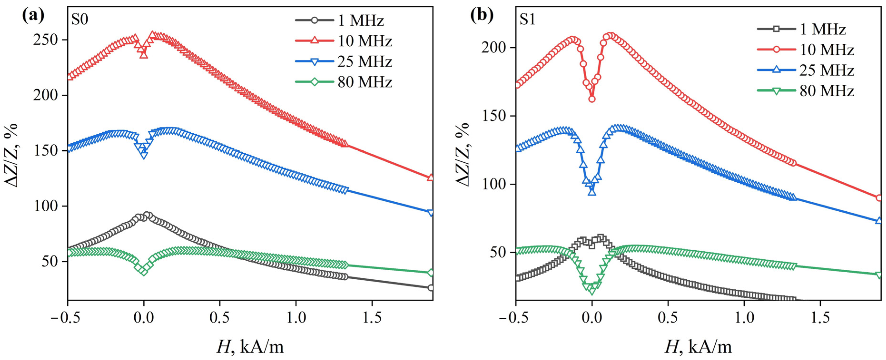
Figure 7.
Frequency dependences of the reduced impedance Z(f)/RDC of the S0 ribbons. The dependences were obtained in magnetic fields of 0 (a) and 12 kA/m (b). Lines are experimental dependences; markers—dependencies restored using MIT. The tables show the magnetic permeability values reconstructed using MIT.
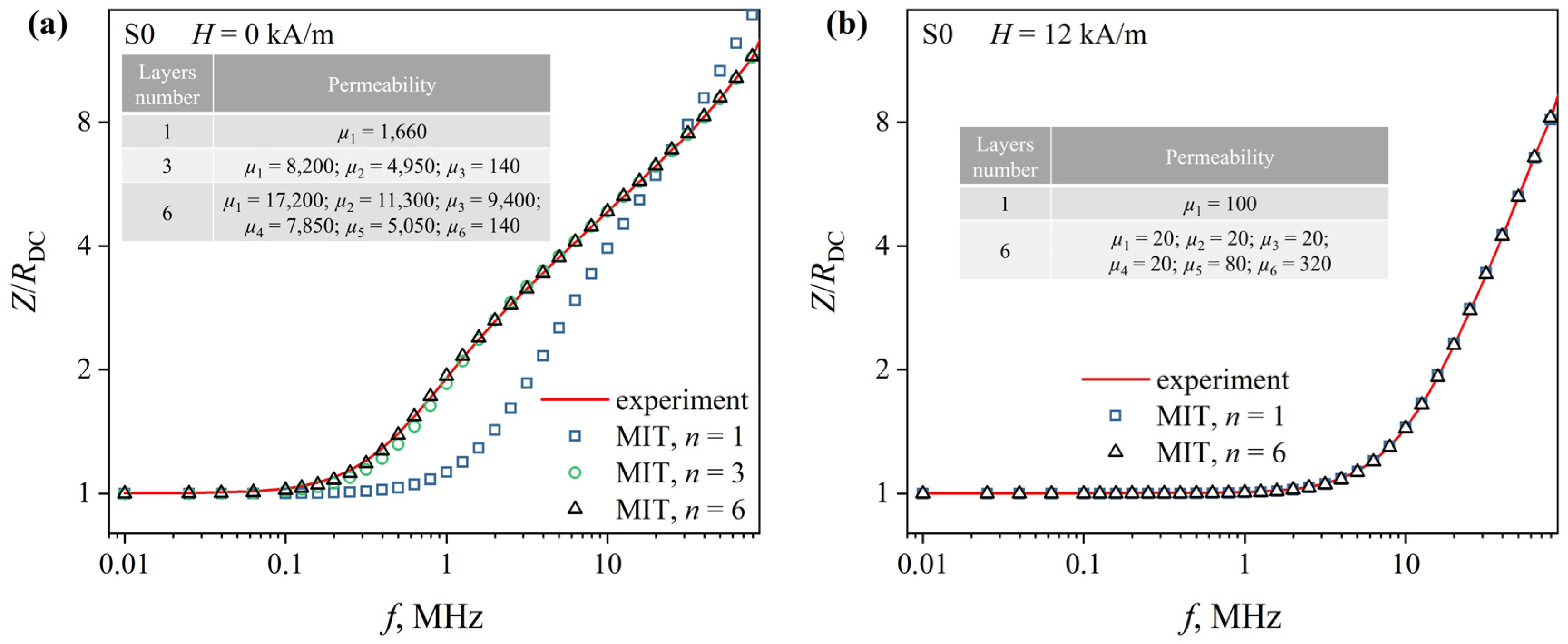
Figure 8.
Frequency dependences of the reduced impedance Z(f)/RDC of the S1 ribbons. The dependences were obtained in magnetic fields of 0 (a) and 12 kA/m (b). Lines are experimental dependences; markers—dependencies restored using MIT. The tables show the magnetic permeability values reconstructed using MIT.

Figure 9.
Distributions of the magnetic permeability over the S0 ribbon cross section in the magnetic fields with strengths (a) 0, 0.02 and 0.26 kA/m and (b) 2.80, 7.6 and 12.4 kA/m.
Figure 9.
Distributions of the magnetic permeability over the S0 ribbon cross section in the magnetic fields with strengths (a) 0, 0.02 and 0.26 kA/m and (b) 2.80, 7.6 and 12.4 kA/m.

Figure 10.
Distributions of magnetic permeability over the S1 ribbon cross section in magnetic fields with strengths (a) 0, 0.06 and 0.32 kA/m and (b) 2.80, 7.6 and 12.4 kA/m.
Figure 10.
Distributions of magnetic permeability over the S1 ribbon cross section in magnetic fields with strengths (a) 0, 0.06 and 0.32 kA/m and (b) 2.80, 7.6 and 12.4 kA/m.

Table 1.
Sample parameters for experimental study.
| Sample | Composition | Length l0, mm | Width a, mm | Thickness 2b, µm | Magnetostriction Sign | Specific Conductivity, kS/m |
|---|---|---|---|---|---|---|
| S0 | Co68.5Fe4.0Si15.0B12.5 | 30 | 0.71 | 24 | − | 615 |
| S1 | Co68.6Fe3.9Mo3.0Si12.0B12.5 | 30 | 0.78 | 26 | + | 618 |
Table 2.
Coordinates of the layers of ribbon models S0 and S1 when performing MIT.
| Sample | Layer Boundary Coordinates, µm | |||||
|---|---|---|---|---|---|---|
| y1 | y2 | y3 | y4 | y5 | y6 | |
| S0 | 4 | 6 | 8 | 10 | 11 | 12 |
| S1 | 4 | 6 | 8 | 10 | 12 | 13 |
Disclaimer/Publisher’s Note: The statements, opinions and data contained in all publications are solely those of the individual author(s) and contributor(s) and not of MDPI and/or the editor(s). MDPI and/or the editor(s) disclaim responsibility for any injury to people or property resulting from any ideas, methods, instructions or products referred to in the content. |
© 2023 by the authors. Licensee MDPI, Basel, Switzerland. This article is an open access article distributed under the terms and conditions of the Creative Commons Attribution (CC BY) license (https://creativecommons.org/licenses/by/4.0/).
Share and Cite
MDPI and ACS Style
Bukreev, D.A.; Derevyanko, M.S.; Semirov, A.V. Magnetoimpedance Effect in Cobalt-Based Amorphous Ribbons with an Inhomogeneous Magnetic Structure. Sensors 2023, 23, 8283. https://doi.org/10.3390/s23198283
AMA Style
Bukreev DA, Derevyanko MS, Semirov AV. Magnetoimpedance Effect in Cobalt-Based Amorphous Ribbons with an Inhomogeneous Magnetic Structure. Sensors. 2023; 23(19):8283. https://doi.org/10.3390/s23198283
Chicago/Turabian StyleBukreev, Dmitry A., Michael S. Derevyanko, and Alexander V. Semirov. 2023. "Magnetoimpedance Effect in Cobalt-Based Amorphous Ribbons with an Inhomogeneous Magnetic Structure" Sensors 23, no. 19: 8283. https://doi.org/10.3390/s23198283
Note that from the first issue of 2016, this journal uses article numbers instead of page numbers. See further details here.