


An Application of Analytic Wavelet Transform and Convolutional Neural Network for Radar Intrapulse Modulation Recognition


Faculty of Mechatronics, Armament, and Aerospace, Military University of Technology, 00-908 Warsaw, Poland
*
Authors to whom correspondence should be addressed.
Sensors 2023, 23(4), 1986; https://doi.org/10.3390/s23041986
Submission received: 14 December 2022
/
Revised: 30 January 2023
/
Accepted: 6 February 2023
/
Published: 10 February 2023
(This article belongs to the Special Issue Radar Signal Detection, Recognition and Identification)
Abstract
:This article analyses the possibility of using the Analytic Wavelet Transform (AWT) and the Convolutional Neural Network (CNN) for the purpose of recognizing the intrapulse modulation of radar signals. Firstly, the possibilities of using AWT by the algorithms of automatic signal recognition are discussed. Then, the research focuses on the influence of the parameters of the generalized Morse wavelet on the classification accuracy. The paper’s novelty is also related to the use of the generalized Morse wavelet (GMW) as a superfamily of analytical wavelets with a Convolutional Neural Network (CNN) as classifier applied for intrapulse recognition purposes. GWT is used to obtain time–frequency images (TFI), and SqueezeNet was chosen as the CNN classifier. The article takes into account selected types of intrapulse modulation, namely linear frequency modulation (LFM) and the following types of phase-coded waveform (PCW): Frank, Barker, P1, P2, and Px. The authors also consider the possibility of using other time–frequency transformations such as Short-Time Fourier Transform(STFT) or Wigner–Ville Distribution (WVD). Finally, authors present the results of the simulation tests carried out in the Matlab environment, taking into account the signal-to-noise ratio (SNR) in the range from −6 to 0 dB.
1. Introduction
Nowadays, Electronic Warfare (EW) is an important element of battlefields. Information about the location of hostile emission sources allows for effective mission planning and ensuring the safety of one’s own resources. At the same time, an increasing number of emissions and extensive research on the implementation of new types of radar waveform [1,2] reflect the complexity of the source identification problem and require the use of flexible solutions allowing for adaptation to changing conditions. For this reason, Artificial Intelligence (AI) algorithms, and in particular Machine Learning (ML) methods, which can be trained with new data appearing during the operations, seem to be an inseparable element of a modern EW system. However, in order for the application of ML to be effective, appropriate analyses and research works related to signal processing and the feature extraction process should be carried out. Recently, the use of TFI obtained with STFT, WVD or continuous wavelet transform (CWT) is often considered [3,4,5,6]. The proposal for a radar signal recognition method based on TFI and high-order spectra analysis is presented in [7].
A very important aspect that should be considered when using TFI for signal recognition algorithms is the analysis of the influence of the type, shape, and length of the window, in the cases of STFT or WVD, or the type and parameters of wavelet in the case of CWT, specifically AWT. Transformation parameters, when selected incorrectly, may significantly affect the classification capabilities. For this reason, in this article, the authors presented their simulation studies related to the influence of generalized Morse wavelet (GMW) parameters on the classification accuracy of the proposed method. This allows to obtain comparable or even higher accuracy than when using WVD, which is currently considered very effective in this respect [6]. At the same time, the use of GWT is characterized by much lower computational complexity, resulting in a reduction in time in both the classification process and the network learning. It is worth noticing that all the simulation tests have been carried out using smoothed pseudo-WVD (SPWVD) with a Kaiser window of various shape parameters ().
The number of algorithms based on TFIs and deep learning proposed in the literature, e.g., [8,9,10] has been dynamically increasing in recent years. However, there is a visible lack of analysis in the field of parameters values selection for proposed time–frequency transforms. The type of applied atom (such as wavelet) or smoothing window used in energy distributions determines the possibility of adjusting to certain characteristics of the signal or the required level of interference reduction. For different parameter values, the same differences are observed in recognition ability for selected waveform types, so it is considered by authors using a set of networks trained with different wavelet types and parameter values and/or adding other methods used for signal recognition purposes and then applying data fusion methods. The problem of intrapulse modulation recognition with a fusion network is presented in [4]. Data fusion techniques are successfully used in areas such as tracking systems [11] or multisensory systems for unnamed aerial vehicles (UAV) detection [12].
An integral part of the EW system is signal intelligence (SIGINT). In the case of communications intelligence (COMINT) systems, the key information is the type and level of the modulation system used by the enemy. Intercepting this information not only enables to identify the source but also facilitates demodulation, decoding, and decryption of the transmitted signal. Typically, the ability to recognize common modulation types such as Phase Shift Keying (PSK), Frequency Shift Keying (FSK), Amplitude Shift Keying (ASK) or Quadrature Amplitude Modulation (QAM) is considered [13,14]. There are also studies taking into account the possibility of detection of OFDM transmission, among other communication signals [15,16]. In the case of electronic intelligence (ELINT), the main task of the system is to detect, classify, and determine the location of the emission sources other than communication. Therefore, these are particularly radars. The structure and parameters of the radar signals depend primarily on their intended use, no matter if they are early warning radars, short-, medium-, and long-range missile systems radars, as well as aircraft radars, jamming systems, or any other. Typical radar waveforms considered in most studies are continuous wave (CW) or pulses with LFM, stepped frequency modulation (SFM), and phase coding (PC) or traditional pulses with no intrapulse modulation applied. However, more complex types of waveform such as those with nonlinear frequency modulation or mixed signals are increasingly being considered [2,16,17].
In ELINT systems, many emission source parameters, such as radio frequency (RF), direction of arrival (DOA), time of arrival (TOA), pulse width (PW), pulse repetition frequency (PRF), intrapulse modulation, etc., are determined. These parameters are stored in the database and constitute the basis of the process of recognizing the emissions detected by the EW system. In order to determine the basic parameters of radar signals, it is necessary to perform signal processing and the selection of features allowing for effective classification. This issue is a dynamically developing area of research [18,19,20,21,22], while measuring the parameters of specific radar signals in real time still remains a challenge.
The radar emission identification process is usually carried out using a knowledge-based approach. In [18], methods for determining specific radar signal parameters (signatures) are discussed. In [20], the authors analyze the role of estimation accuracy of the arrival time of each step of the pulse. As it turns out, it may affect the determination correctness of such parameters as PW and PRF. Moreover, the application of the wavelet transform (WT) as well as Haar wavelet as tools for sorting radar signals has also been proposed. Compared with the traditional pulse repetition interval algorithm based on a statistics histogram, the method based on WT is characterized by the high accuracy of the arrival time. In [19], three characteristic parameters, namely CWT eigenvalue, frequency domain moment kurtosis coefficient, and frequency domain moment skewness coefficient, have been used in order to recognize the radar signal. The following signals have been considered: polynomial phase signal, pseudocode phase modulation and sinusoidal frequency modulation, product composite of pseudocode phase modulation and LFM, and convolution composite of pseudocode phase modulation and LFM. For a signal-to-noise ratio (SNR) higher then 0 dB, the probability of signal recognition is claimed to be greater then 98%.
The aim of this article is to present an algorithm for automatic intrapulse modulation recognition with use of an AWT and CNN. The proposed solution is based on the use of generalized Morse wavelet (GMW) as a superfamily of analytic wavelets. The properties of the GMW are described in Section 2.3. A significant advantage of using CWT for signal recognition purposes is the possibility of using CWT coefficients at individual stages of signal analysis, e.g., to estimate selected parameters of a radar signal. The CWT is successfully used in algorithms for sorting radar pulses and determining parameters such as pulse repetition time (PRT), pulse width (PW) or time of arrival (TOA) [20].
The research presented in the paper brings a new contribution to the area of radar signal recognition techniques with the use of TFI. In particular, the authors consider:
- Using AWT (with GMW applied) for radar intrapulse recognition purposes instead of popular WVD, SPWVD or STFT;
- Performance metrics comparing methods with AWT and SPWVD used as TFI;
- The influence of GMW parameters values on classification accuracy;
- Applying SqueezeNet as a CNN classifier.
A significant part of the conducted simulation works has been focused on the study of the influence of generalized Morse wavelet parameters on the properties of the analyzed method. The simulation results are presented in Section 3. The usefulness of AWT is mainly due to the ability to observe the instantaneous amplitude, phase, and frequency of signals simultaneously. The appropriate selection of the wavelet parameters allows, in turn, to obtain the required resolution in frequency and to emphasize specific features of the analyzed signals. The simulations, necessary to test the proposed method and confirm its potential effectiveness, were carried out in the Matlab environment.
The use of TFI enables the simultaneous observation of signal features corresponding to the nature of changes in amplitude, frequency or phase over time. This allows for the complete or partial replacement of traditionally used features, calculated usually with the use of FFT, higher-order statistics, instantaneous amplitude, frequency and phase parameters, cepstral analysis, phase constellation, frequency histogram, etc. Moreover, the algorithms of time–frequency signal decompositions with lower computational complexity and lower memory requirements are presented in the literature [23,24]. The computational complexity of time–frequency distributions is presented in [25]. CNNs, on the other hand, are successfully used in image recognition. This is the main motivation for authors to use one of them as the classifier. According to the authors’ knowledge, at present, there are CNN implementations with a significantly reduced structure. An example of such a CNN is SqueezeNet, the implementation of which is available in the Matlab environment. The primary advantages of SqueezeNet, according to [26], are, e.g.,:
- More efficient distributed training;
- Feasible FPGA and embedded deployment;
- Less overhead when exporting new models to clients.
The SqueezeNet structure implementation in Matlab is 18 layers deep. The network has an image input size of 227 by 227, so TFIs rescaling must be applied. A comparison of classification accuracy using TFI with other CNN-type structures is presented in [8].
2. Materials and Methods
The number of studies related to the possibility of using ML for signal recognition for electronic warfare and, e.g., cognitive radio, has significantly increased in recent years. When analyzing the literature on signal analysis for ELINT systems, one can see the division of the proposed algorithms into two areas of application. The first one focuses on the analysis of signals, with their duration covering a certain number of symbols or a sequence of radar pulses, and determining their characteristic parameters such as PRI, PW, TOA, etc. [18,20,21,22,27,28]. The second concerns the problem of recognizing intrapulse modulation, which is another important parameter characterizing the [5,29,30] emission source. In both cases, the usefulness of using AI algorithms is emphasized.
There are propositions of algorithms using CWT and ML for recognizing modulations of typical signals used in communications such as ASK, PSK, FSK or QAM [13,14,31,32,33,34]. Moreover, in the field of ELINT, more and more papers are published related to the application of AI for the purpose of recognizing selected types of radar waveforms [3,6,9,10,28,29,35].
Of particular interest is the application of CNNs, where TFIs obtained using STFT, WVD or CWT are fed to the network input. In this context, an important problem that requires special attention is the appropriate selection of the type of transformation and its parameters, so that the input data in the form of TFIs contain features that ensure the required classification accuracy of selected signals. The following subsections present issues related to the usefulness of using CWT to generate TFI and CNN as an classifier of selected pulsed radar signals, with particular emphasis on the influence of the parameters of the generalized Morse wavelet on the classification accuracy.
2.1. Radar Waveforms
Applying the pulse compression technology has resulted in a significant increase in the number of signals used in radar technology. Currently, there is a noticeable increase in the number of research works devoted to specific forms of radar signals [1,2], i.e., more and more complex types of radar waveforms ensuring the best possible resolution in time (range) and Doppler frequency (velocity), as well as a high compression ratio. This involves, among other things, the analysis of the ambiguity function, which is also a very useful way of analyzing signal properties in the time–frequency space.
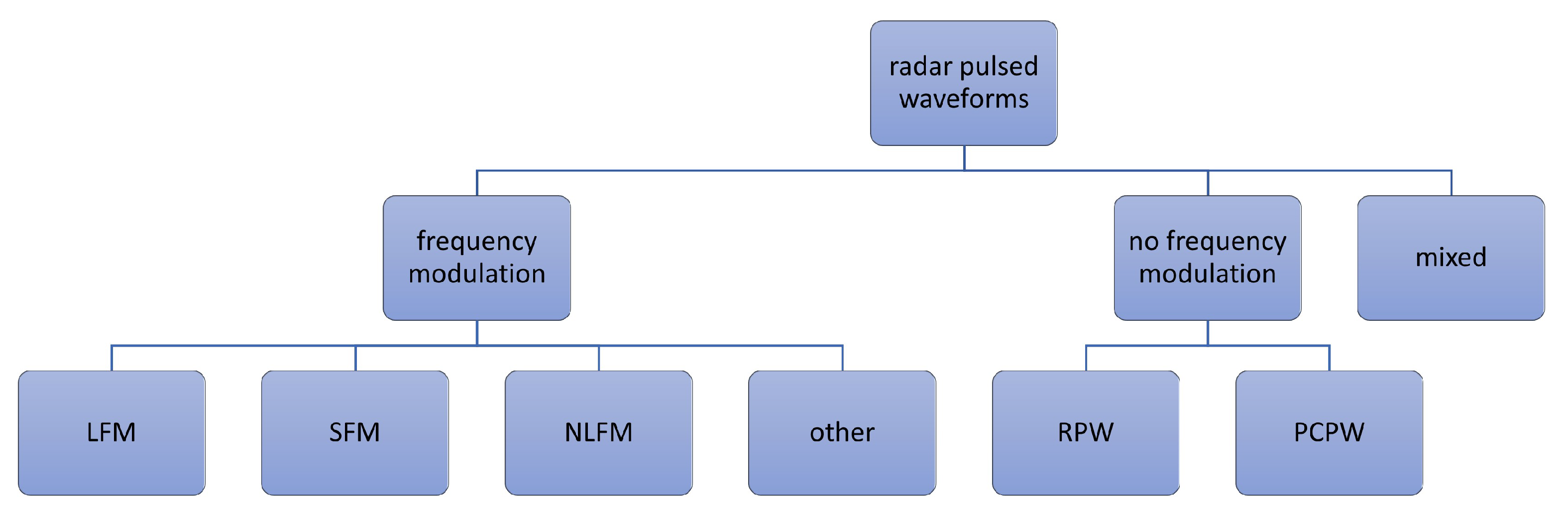
The general division of radar waveforms most often taken into account in the research area for automatic recognition of radar signals is presented in Figure 1. Traditional pulsed radar waveforms include rectangular pulses (RP) with continuous wave (CW), LFM, and phase-coded waveforms (PCW). Other types of often considered radar waveforms are NLFM and SFM.
To an NLFM group of signals, authors also assigned quadratic frequency modulation (QFM), sinusoidal frequency modulation (SiFM), etc. There are also works [15] considering the application of OFDM signals for radar purposes. In [2], there is an algorithm for identifying so-called exotic modulations, which include signals modeled as a combination of LFM and Biphase modulation (BPM). In [30], there is also recognition of the same hybrid waveforms as LFM-BPSK and FSK-BPSK. An analysis of combined signals is also presented in [1], in which authors took into account a group called “mixed”, which includes hybrid modulation types (Figure 1). All listed waveforms can be considered in continuous or pulsed form.
For the purpose of this article, the following types of signals were taken into account for simulation: LFM, RP, and PC waveform. In the studies carried out so far, presented in [31], a significant problem was distinguishing between the different types of signals with phase modulation (PM). In most of the presented research results, the classification accuracy in this group of signals is much worse for both COMINT (M-ary PSK and M-QAM signals) [36] and ELINT (PCW) [37]. In order to emphasize the effectiveness of the proposed method, the following types of codes were included in the phase-coded waveform (PCW) group: Barker, Frank, P1, P2, and Px. According to [38], the complex envelope of the PC pulse, with duration T and M bits in the pulse, is given by equation:
where M is called “chip”, is chip number, , the set of M phases is the phase code associated with , and is a rectangular function. The first family of phase codes taken into account in our research is Barker. There were N = 13 lengths of code chosen for simulations, witch ensures the lowest level of ambiguity function side-lobes () in this code family. There are no longer Barker codes found [39]. The choice of polyphase codes used for simulations (Frank, P1, P2, and Px) is motivated by the fact that difficulties in separating them were expected. The P1, P2, and Px codes are derived from the Frank code [38,39], and they are considered by authors as one family.
The elements of the polyphase codes can be complex depending on the value . For Frank polyphase codes, witch have a length that is perfect square (, where L is integer), the definition of its elements according to [37,38] is
where , and:
According to Equation (2), for , we have phase values:
The Frank, P1, P2, and Px codes are applicable only for perfect square length (). The phase of P1, P2, and Px is given by [37,38]:
only for even L, and:
It should be noted that in the case of the code for even L, takes the values as for the P2 code. For this reason, the simulation parameters should be carefully selected to avoid problems with distinguishing the above codes. For the same reason, the classification was carried out only taking into account the code for odd L. It was show in [37], where for radar waveform recognition purposes Choi–Williams Distribution (CWD) was considered, that P1 and P2 codes get confused with each other. A similar problem was observed in studies where individual levels of PSK were classified for the communication system recognition algorithm [31]. Similarly, it is expected that, in noisy conditions, the differences in this group of phase codes can be blurred.
2.2. The Time–Frequency Transforms in Signal Analysis
Time–frequency (or decomposition) transforms are a very convenient way to present features of different types of waveforms simultaneously in time and frequency domains. The increase in interest in CNNs, particularly observable in the recent years, has made TFIs more and more frequently used schemes in solving the problem of signal classification [3,6]. However, not enough attention is always paid to the influence of the chosen transform parameters on the possibility of enhancing the characteristic features of the signals. This, in turn, may lead to the loss of valuable information and, as a consequence, affect the classification process efficiency. Similarly to the classic approach, the stage of feature extraction determines the effectiveness of the recognition algorithm.
Some of the most popular transforms such as STFT, WVD, and CWT are presented in [40,41]. We can divide them in two classes of solutions: atomic decompositions and energy distributions. The first class includes STFT and CWT, while the second one includes WVD, pseudo-WVD, and SPWVD.
STFT according to [42] is defined as
where is a short time analysis window localized around and . The multiplication by the relatively short window effectively suppresses the signal outside a neighborhood of time point , so the STFT is a “local” spectrum of the signal around t. The time resolution of the STFT is proportional to the effective duration of the analysis window h. In turn, the resolution of the STFT in the frequency is proportional to the effective bandwidth of the analysis window h. According to the above, using the STFT cannot achieve good resolution in time and frequency simultaneously. A good time resolution requires a short window , and a good frequency resolution requires a narrow-band filter, and so a long window .
The CWT of a signal is defined as [42,43]
where the is called mother wavelet and a is the scaling constant. is called baby wavelet and is the translated and scaled version of .
CWT projects a signal on a family of zero-mean functions, called the wavelets, which are translated and dilated versions of the elementary function, called the mother wavelet. When the scale factor is being modified, the duration and the bandwidth of the wavelet are both changed, but its shape remains the same. In contrast to the STFT, which uses a single analysis window, the CWT uses short windows at high frequencies and long windows at low frequencies. This partially overcomes the resolution limitation of the STFT. STFT and CWT are linear transforms of the signal. Another way of signal analysis consists in distributing the energy of the signal along the two variables of time and frequency. This leads to energy time–frequency distributions, which are naturally quadratic transforms of time and frequency. For STFT, we have a spectral energy density of the locally windowed signal , defined as [42,43]
According to Equation (5) spectrogram is a real-valued and non-negative distribution and satisfies the global energy distribution property:
CWT also preserves energy:
The second class of time–frequency representations is energy distributions. Some of the most commonly used energy distributions for signal recognition are WVD and CWD. The WVD is defined as [42]
and is a nonlinear decomposition, so the spectrum of two combined signals is not the sum of their spectra but includes so-called cross-spectrum:
where:
The WVD interference terms will be nonzero regardless of the time–frequency distance between the two signal terms [42]. This could be troublesome and make it difficult to visually interpret the WVD image. A common way to reduce interferences is to use anew distribution, called pseudo-WV, defined as:
where is regular window. The windowing operation is equivalent to frequency smoothing. Another modification of WVD is the smoothed pseudo-Wigner–Ville Distribution (SPWVD), defined as
According to [42], the compromise of the spectrogram between time and frequency resolutions is in case of SPWVD being replaced by a compromise between the joint time–frequency resolution and the level of the interference terms. Stronger smoothing in time and/or frequency runs into poorer resolution in time and/or frequency.
2.3. The Analytic Wavelet Transform (AWT) and Generalized Morse Wavelet (GMW)
The continuous wavelet transform (CWT) enables extraction of transient information associated with amplitude/frequency changes and phase shifts, which are characteristics of modulated signals. According to [45,46], it is generally the most useful to describe oscillatory signals and time-localized events in noisy environment, where 1/s normalization is more appropriate. Taking the above into account, the definition of the CWT of a signal takes the form:
where the is called mother wavelet and a is the scaling constant. is called baby wavelet and is the translated and scaled version of . In this case, rescaling time in the input signal as rescales both the time and the scale of CWT but without changing its magnitude. For analytic wavelets considered in [45,46,47], we have for , which means that wavelets vanish for negative frequencies. The AWT is represented in the frequency domain as
For the analytic wavelet , maximum amplitude occurs in the frequency domain at , which is called the peak frequency. In the case of using an analytic wavelet, such as GMW, there is AWT term used. According to [45], if the value of the wavelet in the peak frequency is set to , then for signal , we obtain result .
During the simulation studies, the generalized Morse wavelet was taken into account. According to [45,47,48], the Morse wavelet is defined as follows:
where is a normalization constant, is the unit step function, and and are parameters controlling the wavelet form. The normalization constant is defined in [47] as
It follows from the analysis presented in [48] that, by varying the and parameters, the generalized Morse wavelets can take a wide variety of forms. For example, the family corresponds to the Cauchy (or Paul) wavelet, the correspond to analytic Derivative of Gaussian wavelets, and corresponds to Airy wavelets family [47].
On Figure 8 and Figure 9 are presented the TFIs of radar signal with Frank code (N = 16), obtained with AWT and Morse wavelet for different values of and and two values for SNR. There is a significant impact of the parameters of the Morse wavelet on the form of CWT and on the way in which TFI is affected by the increased level of noise. On this basis, it can be assumed that a higher accuracy of the classification can be obtained for selected parameters and . The simulation results described in the following subsections confirm the above statement.
3. Results
In order to carry out the research works, the following equipment (hardware and software) was used:
- Dell Precision 3561, i7-1180H, 32GB RAM, NVidia T600, Win11, manufacturer: Dell, Warsaw, Poland;
- MATLAB Version: 9.12.0.2039608 (R2022a) Update 5 with Toolboxes, manufacturer: MathWorks, Inc., Natick, MA, USA.
The simulations were performed for recognition between continuous wave (CW), LFM, and phase-coded waveforms. For signals with phase coding, the same number of chips in one pulse was selected for the Frank, P1, P2 code. Due to the fact that in the Px code for even values of L the phase takes the same values as in P2 code, the L was set to the odd one. The simulation parameters of phase-coded waveforms are listed in Table 1.
The conducted research was based on AWT and the use of the Morse wavelet. The authors focused on the analysis of the impact of the wavelet parameters on the obtained classification accuracy. The general simulation parameters are presented in Table 2.
The simulation tests were carried out taking into account selected values of the parameter, and for each of them, the parameter was changed in the loop. Two parameters per set were considered. The first one was with the analogy with Morse wavelet parameters presented in [45,47,48] and listed in Table 3. Additionally, was applied. The view of the wavelets corresponding to the parameters and from Table 3 is shown in the Figure A1 in Appendix A.
The second wavelet parameters set is presented in Table 4. The number of oscillations and duration of wavelets was increased (according to change in and ) to find out if they could better match the recognized waveform. However, there was no significant increase in classification accuracy noticed.
Only for and , the same small increase in classification accuracy was observed. Lower classification correctness also occurred for the same types of PCW: P1 and P2 codes. Generally, classification accuracy remained at the level of about 85–95% (Table 5).
In spite of the lack of significant improvement, it is worth noticing that frequency resolution is much better for higher wavelet parameters values. This can be useful for frequency-modulated waveform recognition and methods for optimal scale selection for emitter parameters estimation e.g., pulse duration (PD), sweep frequency, pulse repetition interval (PRI), time of arrival (TOA), and others.
The confusion matrix for parameters with the highest total accuracy corresponding to Table 3 is presented in Figure 10. The overall classification accuracy for , was 98.2%.
Additionally, in Figure 11, receiver operating characteristic (ROC) curves for the method with AWT applied (with Morse wavelet parameters: , ) are presented.
The shape of the one-versus-all ROC curve for Barker confirms that their classifier for high-value true positives gives a significant level of false positives, which corresponds to the confusion matrix presented in Figure 10. In the case of Frank, P1, and P2 signals, the one-versus-all ROC curves indicate slightly better performance.
For comparative purposes, the classification process was carried out with SPWVD as TFI and with the Kaiser window with the same parameter values for the smoothing window in frequency and time: window length L = 101 and shape factor N with the selected values. The classification accuracy obtained for each value of N is presented in Table 6.
A similar correctness of the classification was obtained for shape factor N = 1, and the confusion matrix is shown in Figure 12. The overall classification accuracy for shape factor N was 96.3%. Lower classification accuracy occurred for P1 and P2 codes, as well as some problems with distinguishing the waveform with the Barker and Frank code. This is a similar situation as for the method with AWT applied.
Figure 13 presents ROC curves for the method with SPWVD applied. Similarly, as for the method with AWT applied, there are observable levels of false positives for Barker. In the case of Frank, P1, and P2 signals, the one-versus-all ROC curves indicate slightly worse classification possibilities, almost the same as for the method with AWT applied.
4. Conclusions
The actual direction of the research works presented in this paper was drawn in one of our previous works [49]. The method of feature extraction based of AWT seems to be very versatile. The results presented in [31] show that using CWT and artificial neural networks (ANN) performs as an effective way to recognize communication signals such as ASK, PSK, FSK, and QAM. The usefulness of the wavelet transform in signal analysis and the more and more commonly used TFI prompted the authors to verify the possibility of using AWT (with parameterized GMW) in combination with a reduced CNN structure (SqueezeNet). Thus, the conducted research works were focused on the influence of the GMW parameters on classification accuracy. The obtained results confirm the satisfactory effectiveness of the proposed algorithm for SNR in the range from −6 to 0 dB. The highest obtained classification accuracy is for and .
For comparative purposes, the classification process with TFIs based on SPWVD was conducted. It was observed that both algorithms allow for approximate classification accuracy. The advantage of CWT over SPWVD resides in the ability to use a filter bank to improve the efficiency of calculations. On the other hand, for SPWVD, the use of smoothing windows improves the readability of TFI but requires additional time, which was noticed during the simulation tests.
Future work will include the application of a wider range of selected signals with specific parameters such as pulse width, pulse envelope, pulse repetition time, intrapulse modulation, phase coding types, etc. It seems to be reasonable to consider applying adaptive algorithms for wavelet (in CWT/AWT) or smoothing window parameters selection. Another important problem is selecting the type of classifier. Neural network training is a time-consuming process. In the EW systems domain, there is a continuous need for fast methods. Therefore, faster adaptive methods, such as the one presented in [50], even if with relatively lower classification accuracy, are preferable over those that are slower with higher classification rates. Moreover, an interesting alternative worthy of consideration is information fusion methods, referred to in [11], which, apart from the neural-network-based solutions, deliver analytical methods. This may be particularly attractive due to the mentioned speed requirement assessed on the optimizing methods.
Summarizing the presented considerations, the method based on AWT, applied for TFI calculation with the reduced CNN structure (e.g., SqueezeNet), would be more appropriate for hardware implementations then those with STFT or WVD (SPWVD) applied for TFI calculation and with other types of CNN (ResNet, ALexNet, etc.) as classifiers.
Furthermore, by selecting the appropriate wavelet parameters’ values, it is possible to achieve comparable or even better performance test results than those presented in the references.
Author Contributions
Conceptualization, M.W. and K.K.; methodology, M.W. and K.K.; software, M.W.; validation, M.W.; formal analysis, M.W. and K.K.; investigation, M.W.; resources, M.W.; data curation, M.W.; writing—original draft preparation, M.W. and K.K.; writing—review and editing, M.W., K.K. and A.K.; visualization, M.W.; supervision, A.K.; project administration, A.K.; funding acquisition, M.W. All authors have read and agreed to the published version of the manuscript.
Funding
The methods and results presented in this paper have been obtained during research works conducted within the university research project entitled “Selected problems of detection, recognition and classification of signals as well as analysis of imaging and radar data”. This work was financed by the Military University of Technology (Warsaw, PL), in 2022, under research project UGB-778.
Informed Consent Statement
Not applicable.
Data Availability Statement
Not applicable.
Conflicts of Interest
The authors declare no conflict of interest.
Appendix A
Figure A1.
Morse wavelets corresponding to parameters from Table 3 for selected wavelet center frequency.
Figure A1.
Morse wavelets corresponding to parameters from Table 3 for selected wavelet center frequency.

References
- Li, H.; Zhao, J. Analysis of a combined waveform of linear frequency modulation and phase coded modulation. In Proceedings of the 2016 11th International Symposium on Antennas, Propagation and EM Theory (ISAPE), Guilin, China, 18–21 October 2016; pp. 539–541. [Google Scholar] [CrossRef]
- Niranjan, R.; Rao, C.R.; Singh, A. Real-Time Identification of Exotic Modulated Radar Signals for Electronic Intelligence Systems. In Proceedings of the Emerging Trends in Industry 4.0 (ETI 4.0), Raigarh, India, 19–21 May 2021; pp. 1–4. [Google Scholar] [CrossRef]
- Wang, C.; Wang, J.; Zhang, X. Automatic radar waveform recognition based on time-frequency analysis and convolutional neural network. In Proceedings of the IEEE International Conference on Acoustics, Speech and Signal Processing (ICASSP), New Orleans, LA, USA, 5–9 March 2017; pp. 2437–2441. [Google Scholar] [CrossRef]
- Gao, L.; Zhang, X.; Gao, J.; You, S. Fusion Image Based Radar Signal Feature Extraction and Modulation Recognition. IEEE Access 2019, 7, 13135–13148. [Google Scholar] [CrossRef]
- Wei, S.; Qu, Q.; Su, H.; Shi, J.; Zeng, X.; Hao, X. Intra-pulse modulation radar signal recognition based on Squeeze-and-Excitation networks. Signal Image Video Process. 2020, 14, 1133–1141. [Google Scholar] [CrossRef]
- Si, W.; Wan, C.; Deng, Z. Intra-Pulse Modulation Recognition of Dual-Component Radar Signals Based on Deep Convolutional Neural Network. IEEE Commun. Lett. 2021, 25, 3305–3309. [Google Scholar] [CrossRef]
- Ren, M.; Tian, Y. Radar signal cognition based time-frequency transform and high order spectra analysis. In Proceedings of the IEEE International Conference on Signal Processing, Communications and Computing (ICSPCC), Xiamen, China, 22–25 October 2017; pp. 1–4. [Google Scholar] [CrossRef]
- Li, J.; Zhang, H.; Ou, J.; Wang, W. A Radar Signal Recognition Approach via IIF-Net Deep Learning Models. Comput. Intell. Neurosci. 2020, 2020, 8858588. [Google Scholar] [CrossRef]
- Xia, Y.; Ma, Z.; Huang, Z. Over-the-Air Radar Emitter Signal Classification Based on SDR. In Proceedings of the 6th International Conference on Intelligent Computing and Signal Processing (ICSP), Xi’an, China, 9–11 April 2021; pp. 403–408. [Google Scholar] [CrossRef]
- Xu, T.; Darwazeh, I. Deep Learning for Over-the-Air Non-Orthogonal Signal Classification. In Proceedings of the IEEE 91st Vehicular Technology Conference (VTC2020-Spring), Virtual Event, 25–28 May 2020; pp. 1–5. [Google Scholar]
- Krenc, K.; Gradolewski, D.; Dziak, D.; Kawalec, A. Application of Radar Solutions for the Purpose of Bird Tracking Systems Based on Video Observation. Sensors 2022, 22, 3660. [Google Scholar] [CrossRef] [PubMed]
- Dudczyk, J.; Czyba, R.; Skrzypczyk, K. Multi-Sensory Data Fusion in Terms of UAV Detection in 3D Space. Sensors 2022, 22, 4323. [Google Scholar] [CrossRef]
- Hassan, K.; Dayoub, I.; Hamouda, W.; Berbineau, M. Automatic modulation recognition using wavelet transform and neural network. In Proceedings of the 9th International Conference on Intelligent Transport Systems Telecommunications (ITST), Lille, France, 20–22 October 2009; pp. 234–238. [Google Scholar] [CrossRef]
- Hassan, K.; Dayoub, I.; Hamouda, W.; Berbineau, M. Automatic Modulation Recognition Using Wavelet Transform and Neural Networks in Wireless Systems. EURASIP J. Adv. Signal Process. 2010, 2010, 532898. [Google Scholar] [CrossRef]
- Dash, D.; Sa, K.D.; Jayaraman, V. Time Frequency Analysis of OFDM-LFM Waveforms for Multistatic Airborne Radar. In Proceedings of the 2018 Second International Conference on Inventive Communication and Computational Technologies (ICICCT), Coimbatore, India, 20–21 April 2018; pp. 865–870. [Google Scholar] [CrossRef]
- Wang, Y.; Shi, Z.; Ma, X.; Liu, L. A Joint Sonar-Communication System Based on Multicarrier Waveforms. IEEE Signal Process. Lett. 2022, 29, 777–781. [Google Scholar] [CrossRef]
- Leśnik, C. Nonlinear Frequency Modulated Signal Design. Acta Phys. Pol. A 2009, 116, 351. [Google Scholar] [CrossRef]
- Matuszewski, J. The radar signature in recognition system database. In Proceedings of the 19th International Conference on Microwaves, Radar and Wireless Communications, Warsaw, Poland, 21–23 May 2012; pp. 617–622. [Google Scholar] [CrossRef]
- Shi, Q.; Zhang, J. Radar Emitter Signal Identification Based on Intra-pulse Features. In Proceedings of the IEEE 6th Information Technology and Mechatronics Engineering Conference (ITOEC), Chongqing, China, 15–17 September 2022; pp. 256–260. [Google Scholar] [CrossRef]
- Zheng, Z.; Qi, C.; Duan, X. Sorting algorithm for pulse radar based on wavelet transform. In Proceedings of the IEEE 2nd Information Technology, Networking, Electronic and Automation Control Conference (ITNEC), Chengdu, China, 15–17 December 2017; pp. 1166–1169. [Google Scholar] [CrossRef]
- Chan, Y.T.; Plews, J.W.; Ho, K.C. Symbol Rate Estimation by the Wavelet Transform. In Proceedings of the IEEE International Symposium on Circuits and Systems (ISCAS), Hong Kong, China, 12 June 1997; Volume 1, pp. 177–180. [Google Scholar] [CrossRef]
- Gao, Y.; Li, M.; Huang, Z.; Lu, J. A symbol rate estimation algorithm based on Morlet wavelet transform and autocorrelation. In Proceedings of the IEEE Youth Conference on Information, Computing and Telecommunication, Beijing, China, 20–21 September 2009; pp. 239–242. [Google Scholar] [CrossRef]
- O’Toole, J.M.; Boashash, B. Fast and memory-efficient algorithms for computing quadratic time-frequency distributions. Appl. Comput. Harmon. Anal. 2013, 35, 350–358. [Google Scholar] [CrossRef]
- Munoz, A.; Ertle, R.; Unser, M. Continuous wavelet transform with arbitrary scales and O(N) complexity. Signal Process. 2002, 82, 749–757. [Google Scholar] [CrossRef]
- Vishwanath, M.; Owens, R.M.; Irwin, M.J. The computational complexity of time-frequency distributions. In Proceedings of the IEEE Sixth SP Workshop on Statistical Signal and Array Processing, Victoria, BC, Canada, 4–6 October 1992; pp. 444–447. [Google Scholar] [CrossRef]
- Iandola, F.N.; Moskewicz, M.W.; Ashraf, K.; Han, S.; Dally, W.J.; Keutzer, K. SqueezeNet: AlexNet-level accuracy with 50x fewer parameters and <1 MB model size. arXiv 2016, arXiv:1602.07360. [Google Scholar]
- Nedyalko, P.; Jordanov, I.; Roe, J. Radar Emitter Signals Recognition and Classification with Feedforward Networks. Procedia Comput. Sci. 2013, 22, 1192–1200. [Google Scholar] [CrossRef]
- Granger, E.; Rubin, M.A.; Grossberg, S.; Lavoie, P. A What-and-Where fusion neural network for recognition and tracking of multiple radar emitters. Neural Netw. 2001, 14, 325–344. [Google Scholar] [CrossRef]
- Walenczykowska, M.; Kawalec, A. Application of Continuous Wavelet Transform and Artificial Naural Network for Automatic Radar Signal Recognition. Sensors 2022, 22, 7434. [Google Scholar] [CrossRef]
- Zhang, X.; Zhang, J.; Luo, T.; Huang, T.; Tang, Z.; Chen, Y.; Li, J.; Luo, D. Radar Signal Intrapulse Modulation Recognition Based on a Denoising-Guided Disentangled Network. Remote Sens. 2022, 14, 1252. [Google Scholar] [CrossRef]
- Walenczykowska, M.; Kawalec, A. Type of modulation identification using Wavelet Transform and Neural Network. Bull. Pol. Acad. Sci. Tech. Sci. 2016, 64, 257–261. [Google Scholar] [CrossRef]
- Ho, K.C.; Prokopiw, W.; Chan, Y. Modulation identification of digital signals by the wavelet transform. IEE Proc. Radar Sonar Navig. 2000, 147, 169–176. [Google Scholar] [CrossRef]
- Lv, Y.; Liu, Y.; Liu, F.; Gao, J.; Liu, K.; Xie, G. Automatic Modulation Recognition of Digital Signals Using CWT Based on Optimal Scales. In Proceedings of the IEEE International Conference on Computer and Information Technology, Washington, DC, USA, 11–13 September 2014; pp. 430–434. [Google Scholar] [CrossRef]
- Sobolewski, S.; Adams, W.L.; Sankar, R. Universal Nonhierarchical Automatic Modulation Recognition Techniques For Distinguishing Bandpass Modulated Waveforms Based On Signal Statistics, Cumulant, Cyclostationary, Multifractal And Fourier-Wavelet Transforms Features. In Proceedings of the IEEE Military Communications Conference, Baltimore, MD, USA, 6–8 October 2014; pp. 748–753. [Google Scholar] [CrossRef]
- Wang, X.Z. Electronic radar signal recognition based on wavelet transform and convolution neural network. Alex. Eng. J. 2022, 61, 3559–3569. [Google Scholar] [CrossRef]
- Ghodeswar, S.; Poonacha, P.G. An SNR estimation based adaptive hierarchical modulation classification method to recognize M-ary QAM and M-ary PSK signals. In Proceedings of the 3rd International Conference on Signal Processing, Communication and Networking (ICSCN), Chennai, India, 26–28 March 2015; pp. 1–6. [Google Scholar] [CrossRef]
- Lunden, J.; Koivunen, V. Automatic Radar Waveform Recognition. IEEE J. Sel. Top. Signal Process. 2007, 1, 124–136. [Google Scholar] [CrossRef]
- Levanon, N.; Mozeson, E. Phase-Coded Pulse. In Radar Signals; Wiley-Interscience; IEEE Press: Piscataway, NJ, USA, 2004. [Google Scholar] [CrossRef]
- Farnane, K.; Minaoui, K.; Rouijel, A.; Aboutajdine, D. Analysis of the ambiguity function for phase-coded waveforms. In Proceedings of the 2015 IEEE/ACS 12th International Conference of Computer Systems and Applications (AICCSA), Marrakech, Morocco, 17–20 November 2015; pp. 1–4. [Google Scholar] [CrossRef]
- Boggiatto, P.; Cordero, E.; de Gosson, M.; Feichtinger, H.; Nicola, F.; Oliaro, A.; Tabacco, A. Landscapes of Time-Frequency Analysis; Applied and Numerical Harmonic Analysis; Springer International AG: New York, NY, USA, 2019. [Google Scholar]
- Majkowski, A.; Kołodziej, M.; Rak, R. Joint Time-Frequency And Wavelet Analysis-An Introduction. Metrol. Meas. Syst. 2014, 21, 741–758. [Google Scholar] [CrossRef]
- Auger, F.; Flandrin, P.; Goncalves, P.; Lemoine, O. Time—Frequency toolbox for use with MATHLAB. Available online: https://tftb.nongnu.org/tutorial.pdf (accessed on 12 December 2022).
- Addison, P.S. The Illustrated Wavelet Handbook, Introuctory Theory and Applications in Science, Engeneering, Medicine and Finance; Taylor and Francis Group, LLC: New York, NY, USA, 2002. [Google Scholar]
- Rioul, O.; Vetterli, M. Wavelets and signal processing. IEEE Signal Process. Mag. 1991, 8, 14–38. [Google Scholar] [CrossRef]
- Lilly, J.M.; Olhede, S.C. On the Analytic Wavelet Transform. IEEE Trans. Inf. Theory 2010, 56, 4135–4156. [Google Scholar] [CrossRef] [Green Version]
- Lilly, J. Element analysis: A wavelet-based method for analysing time-localized events in noisy time series. Proc. R. Soc. A Math. Phys. Eng. Sci. 2017, 473, 20160776. [Google Scholar] [CrossRef]
- Lilly, J.M.; Olhede, S.C. Higher-Order Properties of Analytic Wavelets. IEEE Trans. Signal Process. 2009, 57, 146–160. [Google Scholar] [CrossRef]
- Lilly, J.M.; Olhede, S.C. Generalized Morse Wavelets as a Superfamily of Analytic Wavelets. IEEE Trans. Signal Process. 2012, 60, 6036–6041. [Google Scholar] [CrossRef]
- Walenczykowska, M.; Kawalec, A. Radar signal recognition using Wavelet Transform and Machine Learning. In Proceedings of the 23rd International Radar Symposium (IRS), Gdansk, Poland, 12–14 September 2022; pp. 492–495. [Google Scholar] [CrossRef]
- Rybak, Ł.; Dudczyk, J. Variant of Data Particle Geometrical Divide for Imbalanced Data Sets Classification by the Example of Occupancy Detection. Appl. Sci. 2021, 11, 4970. [Google Scholar] [CrossRef]
Figure 1.
General division of radar waveforms.

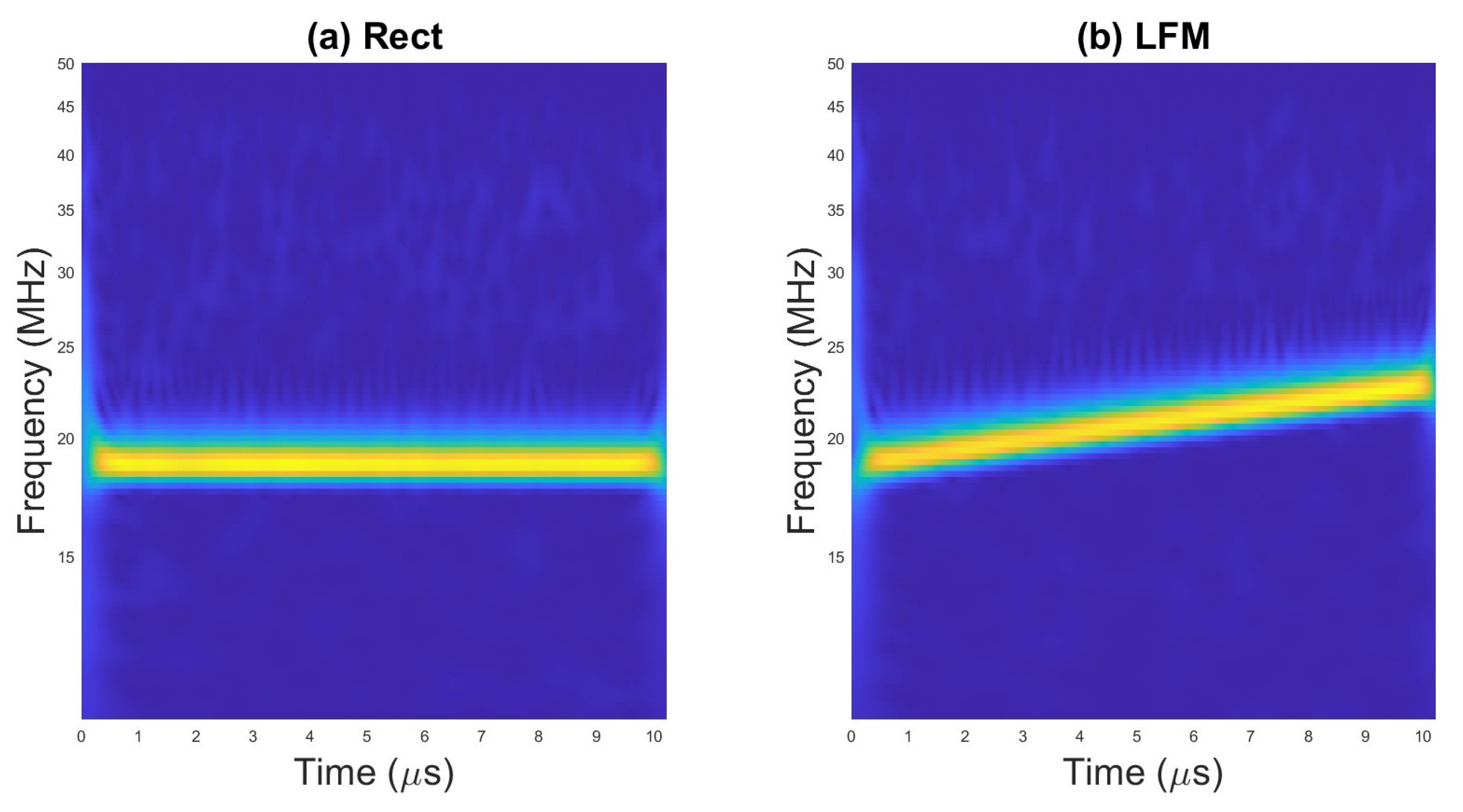
Figure 2.
Scalogram for (a) rectangular pulse and (b) LFM.

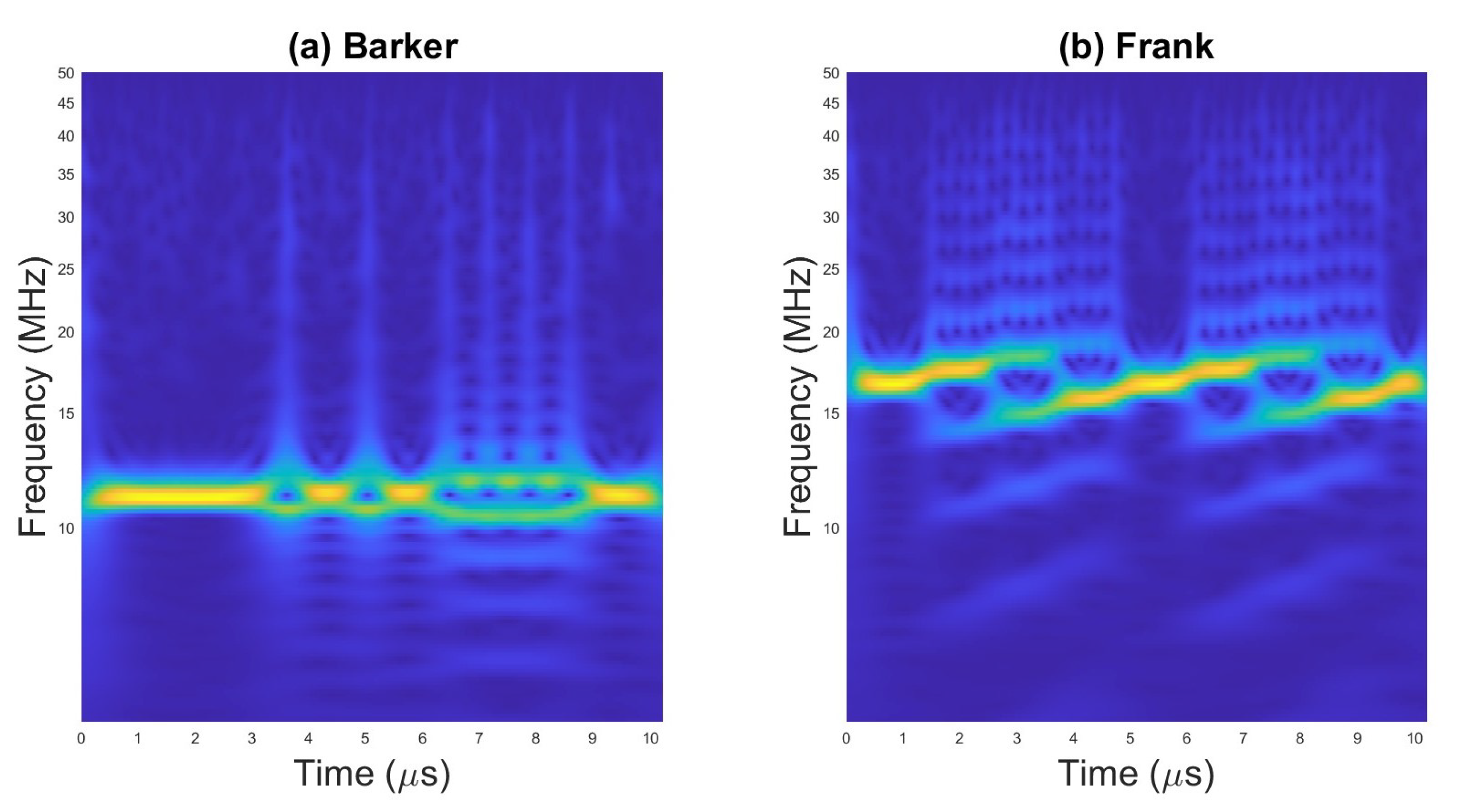
Figure 3.
Scalogram for (a) pulses with Barker code and (b) pulses with Frank code.

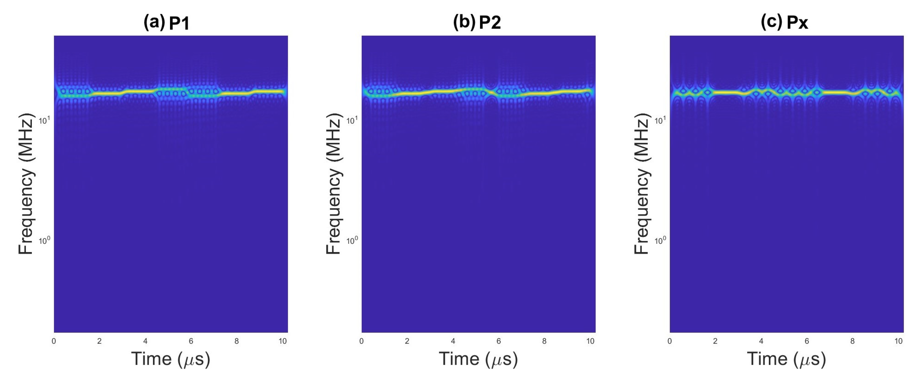
Figure 4.
Scalogram for pulses with (a) P1 code, (b) P2 code, and (c) code.

Figure 5.
WVD for (a) rectangular pulse; (b) LFM.

Figure 6.
WVD for (a) pulse with Barker code; (b) pulses with Frank code.

Figure 7.
WVD for pulses with (a) P1 code, (b) P2 code, and (c) code.

Figure 8.
Scalogram for the pulse with Frank code for SNR = 20 dB.

Figure 9.
Scalogram for the pulse with Frank code for SNR = 0 dB.

Figure 10.
Confusion matrix for AWT with Morse wavelet parameters: , .

Figure 11.
One-versus-all ROC curves for each class for the method with AWT with Morse wavelet parameters: , .
Figure 11.
One-versus-all ROC curves for each class for the method with AWT with Morse wavelet parameters: , .

Figure 12.
Confusion matrix for WVD with Kaiser window parameters L = 101, .

Figure 13.
One-versus-all ROC curves for each class for the method with SPWVD with Kaiser window and .
Figure 13.
One-versus-all ROC curves for each class for the method with SPWVD with Kaiser window and .


Table 1.
Phase-coded waveform parameters.
| Code Name | Chip Number |
|---|---|
| Barker | 13 |
| Frank | 16 |
| P1 | 16 |
| P2 | 16 |
| Px | 9 |
Table 2.
General simulation parameters.
| Parameter Name | Parameter Value |
|---|---|
| Carrier frequency | 16.7 MHz to 20 MHz |
| Sample frequency | 100 MHz |
| Bandwidth (for LFM Waveforms) | from 5 to 6.25 MHz |
| SNR | from −6 to 0 [dB] |
| Rician Channel Parameters | PathDelays [0 1.8 3.4]/Fs, AveragePathGains [0–2–10] |
| Number of pulses in signal | 1–2 |
| Number of samples (in observation window) | 1024 |
| Number of each type of signal | 3000 |
| Number of cycles per phase code (in one Chip) | [7, 8] for Barker, Px, [4, 5] for Frank, P1, P2 |
| Wavelet type | Morse |
Table 3.
The and values taken into account in simulation.
| () | |
|---|---|
| 3 | 9 (3), 27 (9), 81 (27), 120 (40) |
| 9 | 27 (3), 81 (9), 243 (27), 360 (40) |
| 27 | 81 (3), 243 (9), 729 (27), 1080 (40) |
Table 4.
Additional and values taken into account in simulation.
| () | |
|---|---|
| 9 | 81 (9), 99 (11), 117 (13), 135 (15), 153 (17), 171 (19), 189 (21), 207 (23), 225 (25), 243 (27), 261 (29), 279 (31), 297 (33), 315 (35), 333 (37), 351 (39) |
| 27 | 728 (27), 783 (29), 831 (31), 891 (33), 945 (35), 999 (37), 1053 (39) |
| 50 | 1500 (30), 1550 (31), 1600 (32), 1650 (33), 1700 (34), 1750 (35), 1800 (36), 1850 (37), 1900 (38), 1900 (39), 1950 (40) |
Table 5.
Total accuracy for parameters corresponding to Table 3.
Table 5.
Total accuracy for parameters corresponding to Table 3.
| Parameter Value | ||||
|---|---|---|---|---|
| 83.7% | 90.1% | 93.6% | 96.4% | |
| 86.6% | 94.8% | 98.2% | 97.3% | |
| 86.1% | 91.7% | 93.8% | 91.9% |
Table 6.
Total accuracy for parameters for selected values of shape factor N.
| Shape Factor N | 0.5 | 1 | 1.5 | 2 | 3 | 4 | 5 |
|---|---|---|---|---|---|---|---|
| Accuracy [%] | 95.9% | 96.3% | 94.4% | 95.6% | 94.4% | 94.9% | 88.9% |
Table 7.
Classification report of the model with AWT applied (Precision, Recall, and F1-Score).
| Signal Type | Barker | Frank | LFM | P1 | P2 | Px | Rect |
|---|---|---|---|---|---|---|---|
| Precision | 0.9412 | 1 | 1 | 0.9800 | 0.9622 | 1 | 1 |
| Recall | 1 | 0.9373 | 1 | 1 | 0.9796 | 0.9615 | 1 |
| F1-Score | 0.9697 | 0.9677 | 1 | 0.9899 | 0.9708 | 0.9804 | 1 |
Table 8.
Classification report of the model with SPWVD applied (Precision, Recall, and F1-Score).
| Signal Type | Barker | Frank | LFM | P1 | P2 | Px | Rect |
|---|---|---|---|---|---|---|---|
| Precision | 0.8992 | 1 | 1 | 0.9186 | 0.9596 | 1 | 1 |
| Recall | 1 | 0.8850 | 1 | 1 | 0.9143 | 0.9615 | 1 |
| F1-Score | 0.9469 | 0.9390 | 1 | 0.9575 | 0.9364 | 0.9804 | 1 |
Disclaimer/Publisher’s Note: The statements, opinions and data contained in all publications are solely those of the individual author(s) and contributor(s) and not of MDPI and/or the editor(s). MDPI and/or the editor(s) disclaim responsibility for any injury to people or property resulting from any ideas, methods, instructions or products referred to in the content. |
© 2023 by the authors. Licensee MDPI, Basel, Switzerland. This article is an open access article distributed under the terms and conditions of the Creative Commons Attribution (CC BY) license (https://creativecommons.org/licenses/by/4.0/).
Share and Cite
MDPI and ACS Style
Walenczykowska, M.; Kawalec, A.; Krenc, K. An Application of Analytic Wavelet Transform and Convolutional Neural Network for Radar Intrapulse Modulation Recognition. Sensors 2023, 23, 1986. https://doi.org/10.3390/s23041986
AMA Style
Walenczykowska M, Kawalec A, Krenc K. An Application of Analytic Wavelet Transform and Convolutional Neural Network for Radar Intrapulse Modulation Recognition. Sensors. 2023; 23(4):1986. https://doi.org/10.3390/s23041986
Chicago/Turabian StyleWalenczykowska, Marta, Adam Kawalec, and Ksawery Krenc. 2023. "An Application of Analytic Wavelet Transform and Convolutional Neural Network for Radar Intrapulse Modulation Recognition" Sensors 23, no. 4: 1986. https://doi.org/10.3390/s23041986
Note that from the first issue of 2016, this journal uses article numbers instead of page numbers. See further details here.