Robust Cooperative Fault-Tolerant Control for Uncertain Multi-Agent Systems Subject to Actuator Faults

Abstract

This article investigates the robust cooperative fault-tolerant control problem of multi-agent systems subject to mismatched uncertainties and actuator faults. During the design process of the intermediate variable estimator, there is no need to satisfy fault estimation matching conditions, and this overcomes a crucial constraint of traditional observers and estimators. The feedback term of the designed estimator contains the centralized estimation errors and the distributed estimation errors of the agent, and this further improves the design freedom of the proposed estimator. A novel fault-tolerant control protocol is designed based on the fault estimation information. In this work, the bounds of the fault and its derivatives are unknown, and the considered method is applicable to both directed and undirected multi-agent systems. Furthermore, the parameters of the estimator are determined through the resolution of a linear matrix inequality (LMI), which is decoupled by employing coordinate transformation and Schur decomposition. Lastly, a numerical simulation result is used to demonstrate the effectiveness of the proposed method.

1. Introduction

Spawned by the rapid advances in networked systems and distributed cooperation, there has been a flurry of activity on the topic of multi-agent systems (MASs). During the past few years, MASs have found extensive application in both industrial and military domains, such as multi-robot systems [1], satellite formation control [2], sensor networks [3], smart grids [4], flight control systems [5], etc.

As a type of interconnected system, MASs complete control tasks by exchanging information among neighboring agents. However, due to the system configuration and communication topology, a fault occurring in one agent can potentially propagate through the network, affect other agents, or even cause network disruption [6,7,8]. As a result, one specific agent fault could significantly impact MASs, potentially causing agent instability or even a system crash. Indeed, it is essential to highlight that faults may occur more frequently as the number of agents increases and as each agent expands in size and complexity. Furthermore, the security and reliability of MASs become increasingly crucial when they operate in complex and adverse environments.

To ensure the reliable operation of control systems, fault diagnosis has gained widespread attention in recent years and become a key focus of research. Fault diagnosis can be categorized into three main themes: fault detection (FD), fault isolation (FI), and fault estimation (FE) [9,10]. FD and FI primarily serve to detect and determine the location of faults, but they cannot obtain accurate fault information. In contrast, FE can provide detailed information about the shape and size of faults [11]. In general, the more fault information that can be obtained, the higher the fault-tolerant control performance [12]. Recently, a lot of fault estimation methods have been developed, including robust estimators, adaptive observers, sliding-mode controllers, and others [13,14]. However, there has been relatively limited research on fault estimation for MASs. For instance, ref. [15] addressed distributed fault estimation for interconnected systems with actuator faults. A novel distributed FD and FI method was proposed in [16] for heterogeneous MASs. To estimate sensor faults, a category of unknown input observers (UIO) was introduced in [17] by incorporating the system state and fault into a new extended vector. A robust fault estimation method using sliding-mode observers was derived in [18] for linear MASs subject to actuator faults. For the case of nonlinear MASs, an intermediate observer was introduced in [19] for estimating system states and actuator faults. Similar approaches were applied in [20] to construct nonlinear fault estimation observers for nonlinear MASs with sensor faults. In [21], timing FE observers were developed for interconnected systems with both multiplicative and additive actuator faults.

It is noteworthy that the majority of fault estimation methods in the aforementioned studies necessitate knowledge of the upper bound of the fault signal. However, since the bounds of fault information are mostly unknown for most control systems, these methods tend to be conservative in terms of fault estimation performance and applicability. Furthermore, in some existing works, the fault signal is designed as a constant, which is unrealistic since faults occurring in dynamic systems are inevitably influenced by environmental conditions and exhibit dynamic characteristics. Hence, these issues must be taken into consideration in the context of fault estimation for MASs.

Additionally, the fault estimation matching condition, which states that the rank of the product of the system output matrix and the fault distribution matrix should equal the rank of the system output matrix, is necessary for most existing fault estimation protocols. The aforementioned condition exhibits a higher level of conservatism when compared to the strict positivity assumption. In response to these challenges, a pioneering fault estimation method grounded in an intermediate observer was introduced in [22]. Notably, this approach dispenses with the necessity for both the fault estimation matching condition and the strictly positive real assumption.

Fault-tolerance control is the follow-up work of fault estimation. In the study of fault-tolerant control for MASs, there has been significant attention placed on observer-based active fault-tolerant control algorithms. In the process of designing fault-tolerant controllers, understanding the magnitude of the fault is crucial, and this information must be estimated by the constructed observers. For a class of MASs under a directed fixed topology, ref. [23] sidestepped the restriction of the requirement of zero initial conditions in most existing works and pioneered a novel delay-dependent fault-tolerant controller that solves the fault-tolerant constrained consensus problem of MASs in the presence of communication delays and actuator faults. Similarly, in order to sidestep the limitation of zero initial conditions in the $H\infty$ control method, by using disturbance estimation information and a new performance function, ref. [24] designed a disturbance rejection adaptive fault-tolerant constrained consensus algorithm and solved the constraint consensus problem of perturbation-resilient adaptive fault-tolerant multi-agent systems under actuator failures. For linear and Lipschitz non-linear systems, an adaptive fault-tolerant controller utilizing the compensated actuator fault estimation information was proposed in [25] to mitigate adverse effects on consensus tracking. The problem of distributed fault-tolerant control for linear systems was explored in [26]. This approach utilized fuzzy logic systems to approximate unknown non-linear functions and implemented local observers to estimate the system states. In [27], a form of distributed adaptive fault-tolerant control strategy was proposed for linear MASs. This strategy aimed to alleviate the adverse impacts of actuator failures and losses in actuator effectiveness.

However, precise system models are necessary in the aforementioned works. Actually, model uncertainties are inevitable for practical systems and can stem from unknown internal or external noise, environmental influences, poor plant knowledge, and uncertain/slowly varying parameters. For multi-area power systems with actuator failures, ref. [28] considered the influence of uncertainty factors in the fault-tolerant controller and designed a fault-tolerant control scheme considering both multiplicative perturbation and additive perturbations. In [29], radial basis function neural networks (RBFNNs) were used to estimate dynamic uncertainties in the system model to ensure the accuracy of formation control. Similarly, the fuzzy logic method was used in [30] to address the problem of dynamic uncertainty estimation and further improve the accuracy of the proposed formation control algorithm. In [31], a distributed fault diagnosis method was created for a category of uncertain MASs with actuator faults. There was a need to design a state feedback controller ahead of the observer, suggesting the assumption that the full-dimensional state of the system can be measured. This does not align with the conditions observed in practical systems. A fault diagnosis algorithm based on an unknown input observer (UIO) was proposed in [32] for linear uncertain MASs. This work is only applicable to undirected MASs.

Unfortunately, most existing works have paid limited attention to fault estimation for MASs with uncertainties. Moreover, in the majority of these works, especially in the context of SMOs and UIOs, it is essential to fulfill the fault estimation matching condition and determine the bounds of the fault signal. Undoubtedly, these constraints greatly reduce the practicality and generality of traditional fault estimation and fault-tolerant control approaches.

Inspired by the above discussions, in this paper, the fault estimation and fault-tolerant control problem is addressed for a class of MASs with uncertainties. The innovations of this paper are as follows:

(1)

A type of intermediate variable observer has been designed for each agent to estimate the fault and system state information. The fault estimation matching condition is not necessary for this approach, which is also applicable to time-varying faults.

(2)

In the observer design process, both the centralized and distributed estimation errors of the agents are considered, which has the advantages of centralized and distributed structures and can enhance design flexibility and improve estimation performance.

(3)

In the current work, it is not necessary to obtain the bounds of faults and their derivatives. Consequently, the distributed fault estimation method proposed in this paper has great generality and practicality.

(4)

Compared with most existing results, this FE and FTC scheme is suitable for both directed and undirected MASs.

The structure of the paper is as follows. Section 2 gives some basic assumptions and describes the problem considered in this paper. Section 3 and Section 4 present the main theoretical results of this paper, including the construction of the intermediate variable observers and the convergence analysis. Section 5 presents a simulation example to demonstrate the effectiveness of the proposed method. Finally, the concluding remarks are given in Section 6.

Notations: In this article, ${\mathbb{R}}^n$ is the n-dimensional Euclidean spaces and $I_N$ is an identity matrix of size $N\times N$. For a vector $s\in {\mathbb{R}}^n$, $∥s∥$ is the Euclidean norm. For a matrix $\mathcal{D}$, $He\left[\mathcal{D}\right]=\mathcal{D}+{\mathcal{D}}^T$, ${\lambda }_{max}\left(\mathcal{D}\right)$ and ${\lambda }_{min}\left(\mathcal{D}\right)$ represent the maximum and minimum eigenvalues of a matrix $\mathcal{D}$, respectively.

2. Problem Statement

In this section, the problem formulation is presented. Consider the following linear MASs with unknown mismatched uncertainties

$$\left\{\begin{array}{c}{\dot{x}}_i\left(t\right)=(A+\Delta A\left(t\right))x_i\left(t\right)+B{u}_i\left(t\right)+E{f}_i\left(t\right)\hfill \\ y_i\left(t\right)=C{x}_i\left(t\right)\hfill \end{array}\right.$$

(1)

where $x_i\left(t\right)\in {\mathbb{R}}^n$ is the state information of agent i, and $u_i\left(t\right)\in {\mathbb{R}}^m$ and $y_i\left(t\right)\in {\mathbb{R}}^q$ are the control input and measured output of the system. $f_i\left(t\right)\in {\mathbb{R}}^r$ is the fault signal and represents actuator faults when $E=B$. $\Delta A\left(t\right)$ is the perturbed matrix that satisfies $\Delta A\left(t\right)=MF\left(t\right)N$, where $F^T\left(t\right)F\left(t\right)\le I$. A, B, E, and C are the known constant matrices of the system, which have appropriate dimensions. Without loss of generality, in this paper, we assume that $(A,C)$ is observable and $(A,B)$ is stabilizable.

Assumption 1.

In this paper, the fault $f_i\left(t\right)$ satisfies $∥\dot{f_i}\left(t\right)∥⩽\theta$ with $\theta ⩾0$.

Assumption 2.

$rank\left(E\right)=r$.

Assumption 3.

The following equation holds with respect to every complex number s

$$Rank\left[\begin{array}{cc}A-sI& E\\ C& 0\end{array}\right]=n+rank\left(E\right)$$

Assumption 4.

$Rank\left(B,E\right)=rank\left(B\right)$.

Remark 1.

Assumption 1 gives the L-2 norm bounds of the fault and its derivative, which implies that the fault and its derivative are energy-bounded. This assumption is common in the field of FD and FTC [22,33] for estimating time-varying signals. In this paper, it is not necessary to know the specific information about the fault and its derivative bounds, i.e., θ is unknown, making the proposed approach more general than most traditional observers [13,14,17], in which the bounds of faults and their first derivatives must be known.

Remark 2.

It is important to note that Assumption 2 is more common than the fault estimation matching conditions proposed in many existing works. Assumption 3 is natural and pervasive in the majority of published articles that investigate fault detection, isolation, and estimation. This assumption implies that the system $(A,C,E)$ has a constant amount of zeros in the left half-plane. Such a condition finds frequent application in the realms of system control and fault diagnosis.

Remark 3.

Assumption 4 is very common in the existing results of fault-tolerant control, implying that the fault is situated within the channel responsible for controlling the system’s input, and there is a likelihood that it can be mitigated through compensation via the control input.

The following lemma is used for the subsequent work:

Lemma 1

((Young’s Inequality) [19]). For any two vectors, $a\in {\mathbb{R}}^n$ and $b\in {\mathbb{R}}^n$, we have

$$a^{T}b⩽\frac{1}{p}{\alpha }^p{∥a∥}^p+\frac{1}{q}{\alpha }^{-q}{∥a∥}^q$$

where $\alpha >0$, $p>0$, $q>0$, and $pq=p+q$.

In this paper, we design a fault estimator to acquire state information and fault information in real time and use the acquired information to design a fault-tolerant control protocol to compensate for the adverse effects of fault signals on MASs for the purpose of robust fault-tolerant cooperative control for MASs.

3. Intermediate Observer Design

In this subsection, an observer is designed for each agent i. To start with, the following intermediate variable ${\xi }_i\left(t\right)$ is denoted:

$${\xi }_i\left(t\right)=f_i\left(t\right)-\omega E^T{x}_i\left(t\right)$$

(2)

where $\omega$ is an intermediate constant selected based on experience.

From Equations (1) and (2), we have the dynamics of the intermediate variable:

$$\begin{array}{cc}\hfill {\dot{\xi }}_i\left(t\right)=& {\dot{f}}_i\left(t\right)-\omega E^T((A+\Delta A)x_i\left(t\right)+B{u}_i\left(t\right)+E{\xi }_i\left(t\right)+\omega E{E}^T{x}_i\left(t\right))\hfill \end{array}$$

(3)

Based on Equations (1)–(3), the following intermediate variable estimator is designed:

$$\left\{\begin{array}{c}{\dot{\widehat{x}}}_i\left(t\right)=A{\widehat{x}}_i\left(t\right)+B{u}_i\left(t\right)+E{\widehat{f}}_i\left(t\right)+{\rho }_1{L}_1{\Delta }_{1i}+{\rho }_2{L}_2{\Delta }_{2i}\hfill \\ \begin{array}{c}\hfill {\dot{\widehat{\xi }}}_i\left(t\right)=-\omega E^{T}E{\widehat{\xi }}_i\left(t\right)-\omega E^T(A{\widehat{x}}_i\left(t\right)+B{u}_i\left(t\right)+\omega E{E}^T{\widehat{x}}_i\left(t\right))\end{array}\hfill \\ {\widehat{f}}_i\left(t\right)={\widehat{\xi }}_i\left(t\right)+\omega E^T{\widehat{x}}_i\left(t\right)\hfill \\ {\widehat{y}}_i\left(t\right)=C{\widehat{x}}_i\left(t\right)\hfill \end{array}\right.$$

(4)

where ${\widehat{x}}_i\left(t\right)$, ${\widehat{\xi }}_i\left(t\right)$, ${\widehat{f}}_i\left(t\right)$, and ${\widehat{y}}_i\left(t\right)$ are the estimations of $x_i\left(t\right)$, ${\xi }_i\left(t\right)$, $f_i\left(t\right)$, and $y_i\left(t\right)$, respectively.

In addition, ${\Delta }_{1i}$ and ${\Delta }_{2i}$ are defined as

$${\Delta }_{1i}=y_i\left(t\right)-{\widehat{y}}_i\left(t\right)$$

(5)

$${\Delta }_{2i}=\sum _{j=1}^N{a}_{ij}\left[\right(y_i\left(t\right)-{\widehat{y}}_i\left(t\right))-(y_j\left(t\right)-{\widehat{y}}_j\left(t\right))]$$

(6)

which represent the centralized and distributed output estimation errors. $L_1\in {\mathbb{R}}^n$ and $L_2\in {\mathbb{R}}^n$ are the observer gain matrices, which are designed later. The non-negative constants ${\rho }_1$ and ${\rho }_2$ are the corresponding weight values that satisfy $0⩽{\rho }_1⩽1$, $0⩽{\rho }_2⩽1$, and ${\rho }_1+{\rho }_2=0$.

Remark 4.

According to the designed intermediate variable estimator, it can be observed that both the centralized output estimation errors, ${\Delta }_{1i}$, and distributed output estimation errors, ${\Delta }_{2i}$, are taken into account. Here, ${\rho }_1$ and ${\rho }_2$ represent the weights assigned to the centralized and distributed output estimation errors, respectively. The magnitude of these values signifies the extent to which neighboring nodes influence the observer: a smaller ${\rho }_1$ (resulting in a larger ${\rho }_2$) amplifies the impact of neighboring nodes, whereas a larger ${\rho }_1$ (resulting in a smaller ${\rho }_2$) reduces the influence of neighboring nodes. In practice, the choice of ${\rho }_1$ and ${\rho }_2$ could increase the flexibility in designing the observers, and their specific selection should be tailored to the actual operating conditions.

4. Estimation Error Analysis

Denote $e_{x_i}\left(t\right)=x_i\left(t\right)-{\widehat{x}}_i\left(t\right)$, $e_{{\xi }_i}\left(t\right)={\xi }_i\left(t\right)-{\widehat{\xi }}_i\left(t\right)$, and $e_{f_i}\left(t\right)=f_i\left(t\right)-{\widehat{f}}_i\left(t\right)$. Since $e_{f_i}\left(t\right)=e_{{\xi }_i}\left(t\right)+\omega E^T{e}_{x_i}\left(t\right)$, we can obtain the dynamics of the estimation error system as follows:

$$\begin{array}{c}\hfill {\dot{e}}_{x_i}\left(t\right)=(A-{\rho }_{1}LC)e_{x_i}\left(t\right)+E{e}_{{\xi }_i}\left(t\right)+\omega E{E}^T{e}_{x_i}\left(t\right)+\Delta A{x}_i\left(t\right)-{\rho }_2{L}_2{\Delta }_{2i}\end{array}$$

(7)

$$\begin{array}{c}\hfill {\dot{e}}_{{\xi }_i}\left(t\right)=-\omega E^{T}E{e}_{{\xi }_i}\left(t\right)-\omega E^{T}A{e}_{x_i}\left(t\right)-{\omega }^{2}E{E}^{T}E{e}_{x_i}\left(t\right)-\omega E^T\Delta A{x}_i\left(t\right)+{\dot{f}}_i\left(t\right)\end{array}$$

(8)

According to Assumption 4, there exists a matrix $B^{*}$ satisfying $(I-B{B}^{*})E=0$. Based on the fault estimation information, the control protocol proposed in this paper is presented as follows:

$$u_i\left(t\right)=-K\widehat{x_i}\left(t\right)-B^{*}E{\widehat{f}}_i\left(t\right)$$

(9)

where K is designed to guarantee that $A-BK$ is Hurwitz. Substituting Equation (9) into Equation (1), we can obtain

$$\begin{array}{cc}\hfill {\dot{x}}_i\left(t\right)=& (A-BK)x_i\left(t\right)+\Delta A{x}_i\left(t\right)+BK{e}_{x_i}\left(t\right)+E{e}_{{\xi }_i}\left(t\right)+\omega E{E}^T{e}_{x_i}\left(t\right)\hfill \end{array}$$

(10)

From Equations (7), (8) and (10), the global error dynamic is

$$\begin{array}{cc}\hfill \dot{x}\left(t\right)=& (I_N\otimes (A-BK))x\left(t\right)+(I_N\otimes \Delta A)x\left(t\right)+(I_N\otimes BK)e_x\left(t\right)\hfill \\ \hfill & +(I_N\otimes E)e_{\xi }\left(t\right)+(I_N\otimes \omega E{E}^T)e_x\left(t\right)\hfill \end{array}$$

(11)

$$\begin{array}{cc}\hfill {\dot{e}}_x\left(t\right)=& (I_N\otimes (A-{\rho }_1{L}_{1}C))e_x\left(t\right)+(I_N\otimes E)e_{\xi }\left(t\right)+(I_N\otimes \omega E{E}^T)e_x\left(t\right)\hfill \\ \hfill & +(I_N\otimes \Delta A)x\left(t\right)-(L\otimes {\rho }_2{L}_{2}C)e_x\left(t\right)\hfill \end{array}$$

(12)

$$\begin{array}{cc}\hfill {\dot{e}}_{\xi }\left(t\right)=& -(I_N\otimes \omega E^{T}E)e_{\xi }\left(t\right)-(I_N\otimes \omega E^{T}A)e_x\left(t\right)-(I_N\otimes {\omega }^{2}E{E}^{T}E)e_x\left(t\right)\hfill \\ \hfill & -(I_N\otimes \omega E^T\Delta A)x\left(t\right)+\dot{f}\left(t\right)\hfill \end{array}$$

(13)

where $x\left(t\right)={[x_1\left(t\right),x_2\left(t\right),\dots ,x_N\left(t\right)]}^T$, $e_x\left(t\right)={[e_{x_1}\left(t\right),e_{x_2}\left(t\right),\dots ,e_{x_N}\left(t\right)]}^T$, $e_{\xi }\left(t\right)={[e_{{\xi }_1}\left(t\right),e_{{\xi }_2}\left(t\right),\dots ,e_{{\xi }_N}\left(t\right)]}^T$, $f\left(t\right)={[f_1\left(t\right),f_2\left(t\right),\dots ,f_N\left(t\right)]}^T$.

Theorem 1.

Under Assumptions 1–3, the intermediate variable estimator in Equation (4) guarantees that the global error dynamic in Equations (11)–(13) is uniformly ultimately bounded for the given intermediate constant $\omega >0$, ${\epsilon }_i>0$ ($i=1,2,3,4$), and there exists matrix $P_j>0$ ($j=1,2,3$), Q, and a constant $\delta >0$ satisfying the following inequality:

$${\Pi }^i=\left[\begin{array}{cc}{\tilde{\Pi }}_{11}^i& {\tilde{\Pi }}_{12}^i\\ *& {\tilde{\Pi }}_{22}^i\end{array}\right]<0,i=1,2,\dots ,N$$

(14)

where ${\tilde{\Pi }}_{11}^i=\left[\begin{array}{ccc}{\Pi }_{11}^i& {\Pi }_{12}^i& {\Pi }_{13}^i\\ *& {\Pi }_{22}^i& {\Pi }_{23}^i\\ *& *& {\Pi }_{33}^i\end{array}\right]$, with ${\Pi }_{11}^i=He\left[P_{1}A-P_{1}BK\right]+\frac{1}{{\epsilon }_1}{N}^{T}N+\frac{1}{{\epsilon }_2}{N}^{T}N+\frac{1}{{\epsilon }_3}{N}^{T}N$, ${\Pi }_{12}^i=P_{1}BK+\omega P_{1}E{E}^T$, ${\Pi }_{13}^i=P_{1}E$, ${\Pi }_{22}^i=He[(P_{2}A-{\rho }_{1}QC)+\left(\omega P_{2}E{E}^T\right)]+\delta {\rho }_2{\overline{\lambda }}_i{C}^{T}C$, ${\Pi }_{23}^i=P_{2}E-\omega A^{T}E{P}_3-{\omega }^{2}E{E}^{T}E{P}_3$, ${\Pi }_{33}^i=-He\left[\omega P_3{E}^{T}E\right]$, ${\tilde{\Pi }}_{22}^i=\mathrm{diag}\left\{-\frac{1}{{\epsilon }_1},-\frac{1}{{\epsilon }_2},-\frac{1}{{\epsilon }_3},-\frac{1}{{\epsilon }_4}\right\}$, ${\tilde{\Pi }}_{12}^i=\left[\begin{array}{cccc}{P}_{1}M& 0& 0& 0\\ 0& P_{2}M& 0& 0\\ 0& 0& \omega P_3{E}^{T}M& P_3\end{array}\right]$. The observer gain matrices can be designed as $L_1=P_2^{-1}Q$, $L_2=\delta P_2^{-1}{C}^T$.

Proof of Theorem 1.

Choose a Lyapunov function as follows:

$$\begin{array}{cc}\hfill V\left(t\right)=& x^T\left(t\right)(I_N\otimes P_1)x\left(t\right)+e_x^T\left(t\right)(I_N\otimes P_2)e_x\left(t\right)+e_{\xi }^T\left(t\right)(I_N\otimes P_3)e_{\xi }\left(t\right)\hfill \end{array}$$

(15)

According to Equations (11)–(13) and $\Delta A\left(t\right)=MF\left(t\right)N$, one has

$$\begin{array}{cc}\hfill \dot{V}\left(t\right)=& x^T\left(t\right)He\left[I_N\otimes (P_{1}A-P_{1}BK)\right]x\left(t\right)+2x^T(I_N\otimes P_{1}MF\left(t\right)N)x\left(t\right)\hfill \\ \hfill & +2x^T(I_N\otimes P_{1}BK)e_x\left(t\right)+2x^T\left(t\right)(I_N\otimes P_{1}E)e_{\xi }\left(t\right)\hfill \\ \hfill & +2x^T\left(t\right)(I_N\otimes \omega P_{1}E{E}^T)e_x\left(t\right)-2e_{\xi }^T\left(t\right)(I_N\otimes \omega P_3{E}^{T}A)e_x\left(t\right)\hfill \\ \hfill & +e_x^T\left(t\right)He\left[I_N\otimes (P_{2}A-{\rho }_1{P}_2{L}_{1}C)\right]e_x\left(t\right)+e_x^T\left(t\right)He\left[L\otimes (P_{2}A-{\rho }_2{P}_2{L}_{2}C)\right]e_x\left(t\right)\hfill \\ \hfill & +2e_x^T\left(t\right)(I_N\otimes P_{2}E)e_{\xi }\left(t\right)+2e_x^T\left(t\right)(I_N\otimes \omega P_{2}E{E}^T)e_x\left(t\right)\hfill \\ \hfill & -2\omega e_{\xi }^T\left(t\right)(I_N\otimes P_3{E}^{T}MF\left(t\right)N)x\left(t\right)+2e_x^T\left(t\right)(I_N\otimes P_{2}MF\left(t\right)N)x\left(t\right)\hfill \\ \hfill & -2e_{\xi }^T\left(t\right)(I_N\otimes \omega P_3{E}^{T}E)e_{\xi }\left(t\right)-2e_{\xi }^T\left(t\right)(I_N\otimes {\omega }^2{P}_3{E}^{T}E{E}^T)e_x\left(t\right)\hfill \\ \hfill & +2e_{\xi }^T\left(t\right)(I_N\otimes P_3)\dot{f}\left(t\right)\hfill \end{array}$$

(16)

From Lemma 1 and $F\left(t\right)F^T\left(t\right)⩽I$, the following inequalities hold for the positive constants ${\epsilon }_1>0$, ${\epsilon }_2>0$, ${\epsilon }_3>0$, and ${\epsilon }_4>0$:

$$\begin{array}{cc}\hfill 2x^T\left(t\right)& (I_N\otimes P_{1}MF\left(t\right)N)x\left(t\right)\hfill \\ \hfill \le & {\epsilon }_1{x}^T(I_N\otimes P_{1}M){(I_N\otimes P_{1}M)}^{T}x\left(t\right)+\frac{1}{{\epsilon }_1}{x}^T(I_N\otimes N^{T}N)x\left(t\right)\hfill \\ \hfill 2e_x^T\left(t\right)& (I_N\otimes P_2{M}_1{F}_1\left(t\right)N_1)x\left(t\right)\hfill \\ \hfill \le & {\epsilon }_2{e}_x^T\left(t\right)(I_N\otimes P_{2}M)(I_N\otimes M^T{P}_2)e_x\left(t\right)+\frac{1}{{\epsilon }_2}{x}^T\left(t\right)(I_N\otimes N^{T}N)x\left(t\right)\hfill \\ \hfill -2e_{\xi }^T\left(t\right)& (I_N\otimes \omega P_3{E}^{T}MF\left(t\right)N)x\left(t\right)\hfill \\ \hfill \le & {\epsilon }_3{e}_{\xi }^T\left(t\right)(I_N\otimes \omega P_3{E}^{T}M)(I_N\otimes \omega M^{T}E{P}_3)e_{\xi }\left(t\right)+\frac{1}{{\epsilon }_3}{x}^T\left(t\right)(I_N\otimes N^{T}N)x\left(t\right)\hfill \end{array}$$

(17)

Based on Assumption 1, it can be inferred that there exists a scalar ${\theta }_N>0$ such that the following inequality consistently holds:

$$\begin{array}{cc}\hfill 2e_{\xi }^T\left(t\right)(I_N\otimes P_3)\dot{f}\left(t\right)\le & \frac{1}{{\epsilon }_4}{e}_{\xi }^T\left(t\right)(I_N\otimes P_3)(I_N\otimes P_3)e_{\xi }\left(t\right)+{\epsilon }_4{\theta }_N\hfill \end{array}$$

(18)

Furthermore, based on Equations (17) and (18), we have

$$\begin{array}{cc}\hfill \dot{V}\left(t\right)\le & x^T\left(t\right)\left[He[I_N\otimes (P_{1}A-P_{1}BK)]\right]x\left(t\right)+{\epsilon }_1{x}^T\left(t\right)(I_N\otimes P_{1}M{M}^T{P}_1)x\left(t\right)\hfill \\ \hfill & +\frac{1}{{\epsilon }_1}{x}^T\left(t\right)(I_N\otimes N^{T}N)x\left(t\right)+2x^T\left(t\right)(I_N\otimes \omega P_{1}E{E}^T)e_x\left(t\right)\hfill \\ \hfill & +2x^T(I_N\otimes P_{1}BK)e_x\left(t\right)+2x^T\left(t\right)(I_N\otimes P_{1}E)e_{\xi }\left(t\right)\hfill \\ \hfill & +e_x^T\left(t\right)\left[He[I_N\otimes (P_{2}A-{\rho }_{1}QC)]\right]e_x\left(t\right)+e_x^T\left(t\right)\left[(L+L^T)\otimes \left(\delta {\rho }_2{C}^{T}C\right)\right]e_x\left(t\right)\hfill \\ \hfill & +2e_x^T\left(t\right)(I_N\otimes P_{2}E)e_{\xi }\left(t\right)+2e_x^T\left(t\right)(I_N\otimes \omega P_{2}E{E}^T)e_x\left(t\right)\hfill \\ \hfill & +{\epsilon }_2{e}_x^T\left(t\right)(I_N\otimes P_{2}M{M}^T{P}_2)e_x\left(t\right)+\frac{1}{{\epsilon }_2}{x}^T\left(t\right)(I_N\otimes N^{T}N)x\left(t\right)\hfill \\ \hfill & -2e_{\xi }^T\left(t\right)(I_N\otimes \omega P_3{E}^{T}E)e_{\xi }\left(t\right)-2e_{\xi }^T\left(t\right)(I_N\otimes \omega P_3{E}^{T}A)e_x\left(t\right)\hfill \\ \hfill & -2e_{\xi }^T\left(t\right)(I_N\otimes {\omega }^2{P}_3{E}^{T}E{E}^T)e_x\left(t\right)+{\epsilon }_3{e}_{\xi }^T\left(t\right)(I_N\otimes {\omega }^2{P}_3{E}^{T}M{M}^{T}E{P}_3)e_{\xi }\left(t\right)\hfill \\ \hfill & +\frac{1}{{\epsilon }_3}{x}^T\left(t\right)(I_N\otimes N^{T}N)x\left(t\right)+\frac{1}{{\epsilon }_4}{e}_{\xi }^T\left(t\right)(I_N\otimes P_3{P}_3)e_{\xi }\left(t\right)+{\epsilon }_4{\theta }_N\hfill \end{array}$$

(19)

where $Q=P_2{L}_1$, $L_2=\delta P_2^{-1}{C}^T$.

Obviously, Equation (19) is equivalent to

$$\dot{V}\left(t\right)\le {\tilde{x}}^T\left(t\right)\Phi \tilde{x}\left(t\right)+{\epsilon }_4{\theta }_N$$

(20)

where

$$\tilde{x}\left(t\right)=\left[\begin{array}{c}x\left(t\right)\\ e_x\left(t\right)\\ e_{\xi }\left(t\right)\end{array}\right],\Phi =\left[\begin{array}{ccc}{\Phi }_{11}& {\Phi }_{12}& {\Phi }_{13}\\ *& {\Phi }_{22}& {\Phi }_{23}\\ *& *& {\Phi }_{33}\end{array}\right]$$

(21)

and ${\Phi }_{11}=He[I_N\otimes (P_{1}A-P_{1}BK)]+{\epsilon }_1(I_N\otimes P_{1}M{M}^T{P}_1)+\frac{1}{{\epsilon }_1}(I_N\otimes N^{T}N)+\frac{1}{{\epsilon }_2}(I_N\otimes N^{T}N)+\frac{1}{{\epsilon }_3}(I_N\otimes N^{T}N)$, ${\Phi }_{12}=(I_N\otimes P_{1}BK)+(I_N\otimes \omega P_{1}E{E}^T)$, ${\Phi }_{13}=(I_N\otimes P_{1}E)$, ${\Phi }_{22}=He[(I_N\otimes (P_{2}A-{\rho }_{1}QC))+(I_N\otimes \omega P_{2}E{E}^T)]+(L+L^T)\otimes \left(\delta {\rho }_2{C}^{T}C\right)+(I_N\otimes P_{2}M{M}^T{P}_2)$, ${\Phi }_{23}=(I_N\otimes P_{2}E)-(I_N\otimes \omega A^{T}E{P}_3)-(I_N\otimes {\omega }^{2}E{E}^{T}E{P}_3)$, ${\Phi }_{33}=-He\left[(I_N\otimes \omega P_3{E}^{T}E)\right]+{\epsilon }_3(I_N\otimes {\omega }^2{P}_3{E}^{T}M{M}^{T}E{P}_3)+{\epsilon }_4(I_N\otimes P_3{P}_3)$.

From Equation (15), we can be obtain

$$\begin{array}{cc}\hfill V\left(t\right)& \le max\left[{\lambda }_{max}\left(P_1\right),{\lambda }_{max}\left(P_2\right),{\lambda }_{max}\left(P_3\right)\right]{(\Vert x\left(t\right)\Vert }^2+{∥e_x\left(t\right)∥}^2+{∥e_{\xi }\left(t\right)∥}^2)\hfill \\ \hfill & =max\left[{\lambda }_{max}\left(P_1\right),{\lambda }_{max}\left(P_2\right),{\lambda }_{max}\left(P_3\right)\right]{∥e_{\tilde{x}}\left(t\right)∥}^2\hfill \end{array}$$

(22)

It follows that

$${∥e_{\tilde{x}}\left(t\right)∥}^2\ge \frac{V\left(t\right)}{max\left[{\lambda }_{max}\left(P_1\right),{\lambda }_{max}\left(P_2\right),{\lambda }_{max}\left(P_3\right)\right]}$$

(23)

From Equation (20), we can obtain

$$\dot{V}\left(t\right)\le {\lambda }_{max}\left(\Phi \right){∥e_{\tilde{x}}\left(t\right)∥}^2+{\epsilon }_4{\theta }_N$$

(24)

It is obvious that ${\lambda }_{max}\left(\Phi \right)<0$, and then we have

$$\dot{V}\left(t\right)\le \kappa V\left(t\right)+\alpha$$

(25)

where $\kappa =\frac{{\lambda }_{max}\left(\Phi \right)}{max\left[{\lambda }_{max}\left(P_1\right){\lambda }_{max}\left(P_2\right),{\lambda }_{max}\left(P_3\right)\right]}<0$, $\alpha ={\epsilon }_4{\theta }_N$.

Denote a set $\Omega$ satisfying the following condition:

$$\begin{array}{c}\hfill \Omega =\{\left(x\left(t\right),e_x\left(t\right),e_{\xi }\left(t\right)\right)\mid {\lambda }_{min}\left(P_1\right)\parallel x\left(t\right){\Vert }^2+{\lambda }_{min}\left(P_2\right)\parallel e_x\left(t\right){\parallel }^2+{\lambda }_{min}\left(P_3\right)\parallel e_{\xi }\left(t\right){\parallel }^2\le -\frac{\alpha }{\kappa }\}\end{array}$$

(26)

Let $\overline{\Omega }$ be the supplementary set of $\Omega$, and then the following inequality holds:

$$\begin{array}{cc}\hfill V\left(t\right)& \ge {\lambda }_{min}\left(P_1)\right.∥{x\left(t\right)\Vert }^2+{\lambda }_{min}\left(P_2\right){∥e_x\left(t\right)∥}^2+{\lambda }_{min}\left(P_3\right){∥e_{\xi }\left(t\right)∥}^2\ge -\frac{\alpha }{\kappa }\hfill \end{array}$$

(27)

if $\left(x\left(t\right),e_x\left(t\right),e_{\xi }\left(t\right)\right)\in \overline{\Omega }$. From Equations (25) and (27), it is obvious that for $\left(x\left(t\right),e_x\left(t\right),e_{\xi }\left(t\right)\right)\in \overline{\Omega }$, we have

$$\dot{V}\left(t\right)\le 0$$

(28)

which means that $\left(x\left(t\right),e_x\left(t\right),e_{\xi }\left(t\right)\right)$ is uniformly ultimately bounded and converges to $\Omega$ exponentially with a rate greater than $e^{\alpha t}$ from the Lyapunov stability theory.

Obviously, the inequality $\Phi <0$ is a preliminary condition to ensure the stability of the global error dynamic in Equations (11)–(13). However, it is not hard to find that $\Phi <0$ is still a high-dimensional and nonlinear characteristic. Therefore, in order to further ensure the solvability of the inequality $\Phi <0$, this condition needs to be further transformed. Note that the term $L+L^T$ in Equation (21) is real symmetric, which means that it must have N real eigenvalues. By spectral decomposition of the real symmetric matrix $L+L^T$, we obtain

$$L+L^T=\overline{V}\overline{\Lambda }{\overline{V}}^T$$

(29)

where $\overline{V}$ is constructed from the eigenvectors of $L+L^T$, and $\overline{\Lambda }=\mathrm{diag}\left\{{\overline{\lambda }}_1,{\overline{\lambda }}_2,\dots ,{\overline{\lambda }}_N\right\}$ and ${\overline{\lambda }}_i(i=1,2,\dots ,N)$ are the corresponding eigenvalues of $L+L^T$. Certainly, the matrix $\overline{V}$ is orthogonal. Then, an orthogonal transformation matrix is defined as follows:

$$\mathcal{H}=\left[\begin{array}{ccc}{\overline{V}}^T\otimes I_n& 0& 0\\ 0& {\overline{V}}^T\otimes I_n& 0\\ 0& 0& {\overline{V}}^T\otimes I_r\end{array}\right]$$

(30)

By pre-multiplying and post-multiplying $\Phi <0$ with $\mathcal{H}$ and its transpose, we can obtain

$$\tilde{\Phi }=\left[\begin{array}{ccc}{\Phi }_{11}& {\Phi }_{12}& {\Phi }_{13}\\ *& {\tilde{\Phi }}_{22}& {\Phi }_{23}\\ *& *& {\Phi }_{33}\end{array}\right]<0$$

(31)

where ${\tilde{\Phi }}_{22}=He[(I_N\otimes (P_{2}A-{\rho }_1{Q}_{2}C))+(I_N\otimes \omega P_{2}E{E}^T)]+\overline{\Lambda }\otimes \left(\delta {\rho }_2{C}^{T}C\right)+I_N\otimes P_2{M}_1{M}_1^T{P}_2$, and it can be found that the other terms are the same as in Equation (21). Finally, based on the Schur complement lemma, it can be found that $\tilde{\Phi }<0$ is equivalent to Equation (14) for $i=1,2,\dots ,N$. The proof of the theorem is complete. □

Remark 5.

In fact, excessively high dimensionality can negatively affect the accuracy of the LMI solution and may even result in no feasible solution for the LMI. Therefore, decoupling and dimension reduction for the preliminary condition $\Phi <0$ is very necessary.

Remark 6.

According to Equations (11)–(13), it can be found that there is a coupling between $x\left(t\right)$, $e_x\left(t\right)$, and $e_{\xi }\left(t\right)$. In order to prove the convergence of the system state and the observation error at the same time, it is necessary to choose a Lyapunov function containing $x\left(t\right)$, $e_x\left(t\right)$, and $e_{\xi }\left(t\right)$.

Remark 7.

In the proof of Theorem 1, by considering the term $e_x^T\left(t\right)\left[(L+L^T)\otimes \left(\delta {\rho }_2{C}^{T}C\right)\right]e_x\left(t\right)$ in Equation (20), it is found that $L+L^T$ is a real symmetric matrix, that is, the Laplacian matrix $\mathcal{L}$ of MASs can be asymmetric. In other words, the topology of MASs can be either undirected or directed in this paper. Therefore, the method proposed in this paper has better universality and practicability compared with most existing results.

Remark 8.

In this paper, the system state and the estimation error are analyzed strictly for convergence, and the explicit boundary, $-\frac{\alpha }{\kappa }$, is obtained. Obviously, by adjusting the gain matrix K, parameters ω, and ${\epsilon }_j(j=1,2,3,4)$, parameter α is sufficiently large, and thus a relatively small bound is obtained. In addition, it is not difficult to find the convergence rate of the system state, and the global error dynamic in Equations (11)–(13) can be quantified by directly selecting the proper matrix K and parameter ω. Once the matrix K and parameter ω are determined, the observer gain matrices, $L_1$ and $L_2$, can be obtained by solving the LMI in Equation (14). At the same time, the feasibility of the LMI in Equation (14) can be enhanced by adjusting parameters ${\epsilon }_j(j=1,2,3,4)$. On the other hand, if the LMI in Equation (14) has a feasible solution, the estimation and control performance can be enhanced by adjusting the matrix K and parameter ω. Therefore, this paper makes full use of the design freedom of parameters to ensure feasibility and effectiveness.

5. Numerical Simulation

In this section, a numerical simulation is used to demonstrate the effectiveness of the method proposed in this paper.

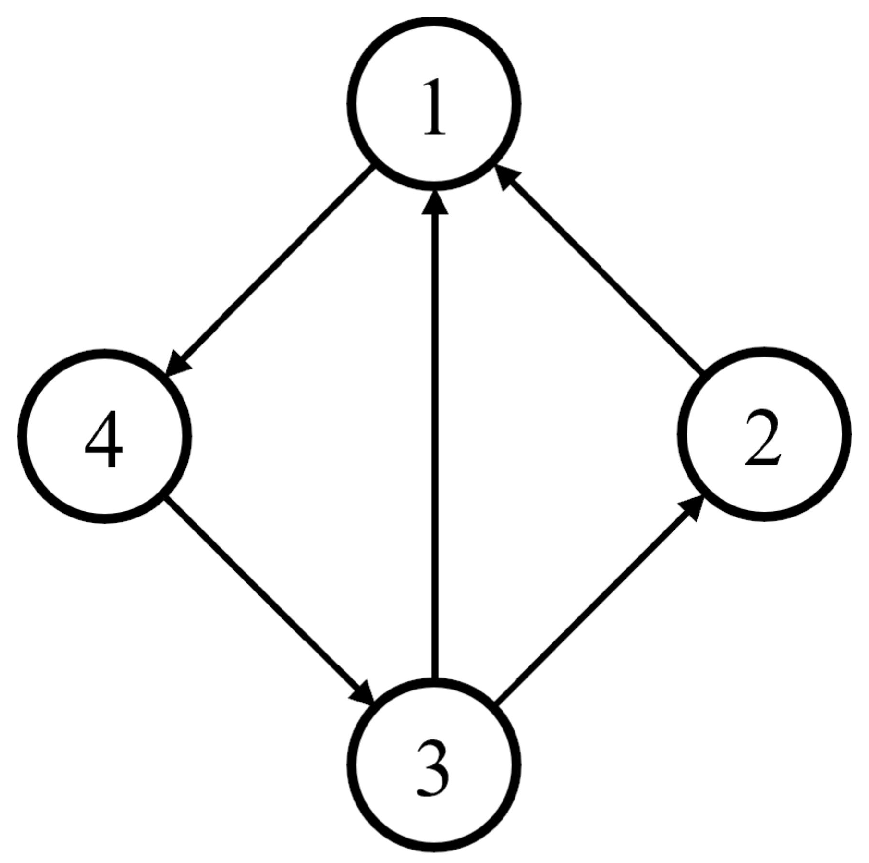
In this numerical simulation, a MAS with four agents is considered. The topology of the MAS is shown in Figure 1.

According to Figure 1, the adjacency matrix $\mathcal{A}$ and the Laplacian matrix $\mathcal{L}$ of the MAS are as follows.

$$\mathcal{A}=\left[\begin{array}{cccc}0& 0& 0& 1\\ 1& 0& 0& 0\\ 1& 1& 0& 0\\ 0& 0& 1& 0\end{array}\right],\mathcal{L}=\left[\begin{array}{cccc}1& 0& 0& -1\\ -1& 1& 0& 0\\ -1& -1& 2& 0\\ 0& 0& -1& 1\end{array}\right]$$

Obviously, since we consider a directed graph, the Laplacian matrix $\mathcal{L}$ is not symmetric.

In this paper, the actuator fault is considered. The system parameters of the ith $(i=1,2,3,4)$ agent are given as

$$A=\left[\begin{array}{ccc}-1& -2& -3\\ -2& -2& 1\\ -3& 1& 1\end{array}\right],B=E=\left[\begin{array}{c}0\\ 0\\ -2\end{array}\right],C=\left[\begin{array}{ccc}1& 0& 0\\ 0& 1& 0\end{array}\right]$$

$$M=\left[\begin{array}{ccc}1& 0& 0\\ 0& 1& 0\\ 0& 0& 1\end{array}\right],N=\left[\begin{array}{ccc}0.5& 0& 0\\ 0& 0.2& 0\\ 0& 0& 0.1\end{array}\right],F\left(t\right)=sin\left(t\right)$$

Obviously, it is not hard to find that $rank\left(CE\right)\ne rank\left(E\right)$, that is, the fault estimation matching condition is not satisfied. In order to make the matrices $(A-BK)$ Hurwitz, the gain matrix K is chosen as $K=\left[\begin{array}{ccc}7.1153& -4.6538& -7.50\end{array}\right]$.

Without loss of generality, we make the following assumptions about the fault of each of the four agents, respectively:

$$f_1\left(t\right)=\left\{\begin{array}{cc}0& 0s⩽t⩽10s\\ sin\left(0.5t\right)+cos\left(0.2t\right)& 10s<t⩽100s\end{array}\right.$$

$$f_2\left(t\right)=\left\{\begin{array}{cc}0& 0s⩽t⩽20s\\ 0.1t-2& 20s<t⩽60s\\ 0.1t-5& 60s<t⩽100s\end{array}\right.$$

$$f_3\left(t\right)=\left\{\begin{array}{cc}0& 0s⩽t⩽30s\\ 2\left(1-e^{-\left(t-30\right)}\right)& 30s<t⩽60s\\ 1-2\left(1-e^{-\left(t-60\right)}\right)& 60s<t⩽100s\end{array}\right.$$

$$f_4\left(t\right)=\begin{array}{cc}0& 0s⩽t⩽100s\end{array}$$

Based on the fault estimator given in the previous section, we choose the weight values as ${\rho }_1=0.3$ and ${\rho }_2=0.7$, respectively. The intermediate constant $\omega$ in Equation (2) is selected as $\omega =0.2$. Based on Theorem 1, the gain matrices of the intermediate variable estimator in Equation (4) can be expressed as follows:

$$L_1=\left[\begin{array}{cc}17.5310& -3.9315\\ -32.1705& 2.0079\\ 69.3836& -66.3622\end{array}\right],L_2=\left[\begin{array}{cc}-0.0261& -0.3609\\ 0.0088& 0.4167\\ -0.9831& -2.3536\end{array}\right]$$

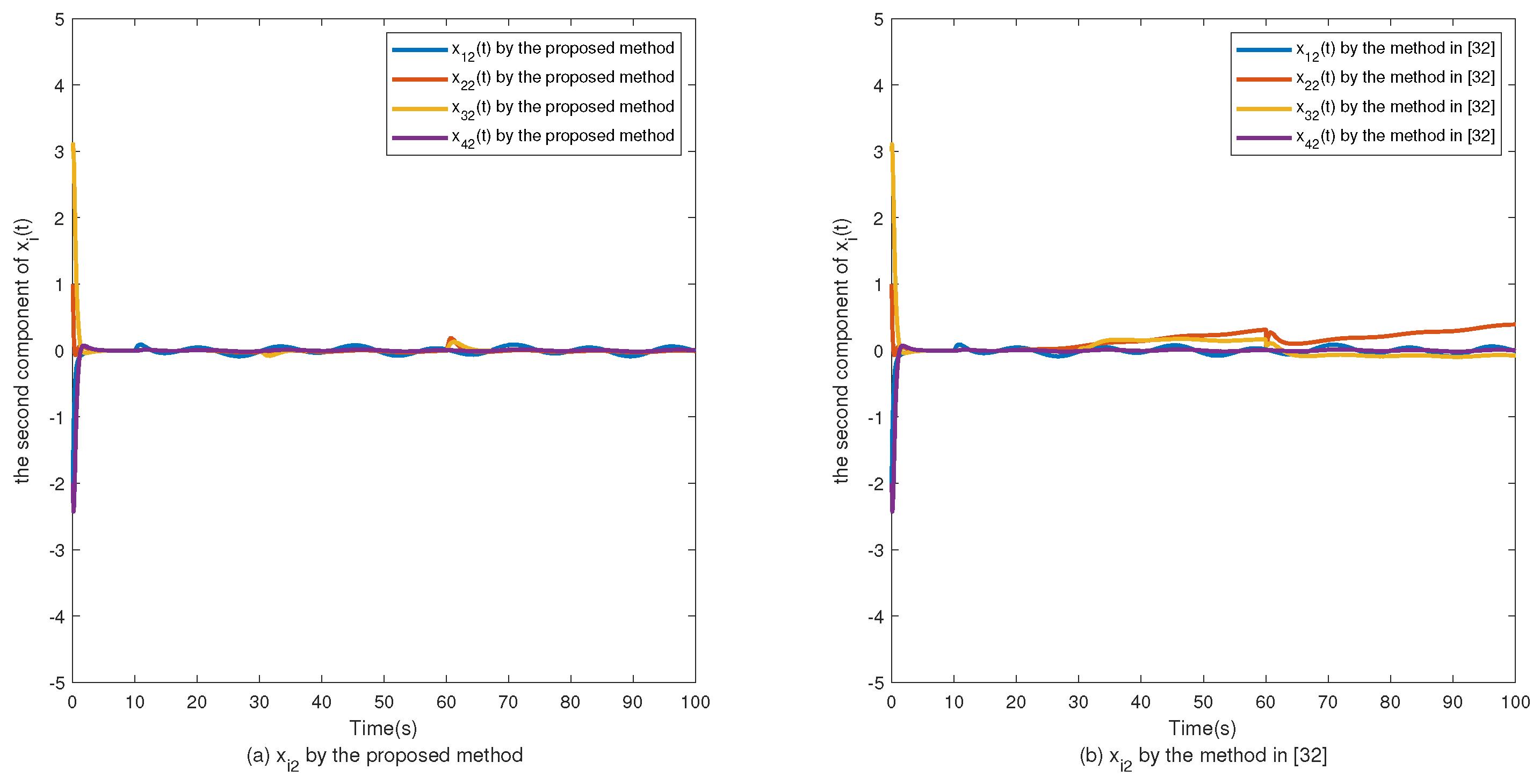
The simulation results are shown in Figure 2, Figure 3, Figure 4, Figure 5, Figure 6, Figure 7 and Figure 8. Figure 2, Figure 3, Figure 4 and Figure 5 show the effectiveness of fault estimation for the actuators of the four agents, respectively, where the red dashed line represents the result of the proposed method and the blue dashed line represents the result of the method proposed in [32]. As can be seen in Figure 2, Figure 3, Figure 4 and Figure 5, the fault estimation results of all agents are more satisfactory. Figure 6, Figure 7 and Figure 8 validate the efficacy of the fault-tolerant control protocol presented in this paper, and the results are better than those of the method proposed in [32]. Obviously, the state component of each agent converges to a small enough range under the designed fault-tolerant control protocol, and the influence of the actuator fault on the convergence process is greatly reduced. In addition, it is found that the fault estimation matching condition of fault estimation is not satisfied, and the bounds of the fault and its derivatives are not required. Therefore, the distributed fault estimation method based on the intermediate variable observer and the fault-tolerant control protocol based on fault estimation proposed in this paper are validated on a MAS with uncertainty.

6. Conclusions

In this paper, a novel robust distributed cooperative fault-tolerant control protocol is designed for a class of MASs with uncertainty and actuator faults. Unlike most existing approaches, in our method, the fault estimation matching condition is not necessary, and the bounds of the fault and its derivative are unknown. By introducing an intermediate variable and using both the centralized estimation errors and distributed estimation errors, the actuator fault is estimated, providing the basis for the fault-tolerance control scheme. Coordinate transformation and Schur decomposition are used to further reduce and decouple the LMI with high dimension and interference coupling, based on which the gain matrix of the estimator can be guaranteed. In future work, distributed cooperative fault-tolerant control for MASs with uncertainties in output and control input channels will be further considered.

References

- Dunbabin, M.; Marques, L. Robots for environmental monitoring: Significant advancements and applications. IEEE Robot. Autom. Mag. 2012, 19, 24–39. [Google Scholar] [CrossRef]
- Kamel, M.A.; Yu, X.; Zhang, Y. Formation control and coordination of multiple unmanned ground vehicles in normal and faulty situations: A review. Annu. Rev. Control 2020, 49, 128–144. [Google Scholar] [CrossRef]
- Chen, F.; Ren, W. On the control of multi-agent systems: A survey. Found. Trends Syst. Control 2019, 6, 339–499. [Google Scholar] [CrossRef]
- Loia, V.; Vaccaro, A. Decentralized economic dispatch in smart grids by self-organizing dynamic agents. IEEE Trans. Syst. Man Cybern. Syst. 2013, 44, 397–408. [Google Scholar] [CrossRef]
- Chang, J.; Guo, Z.; Cieslak, J.; Henry, D. Robust fault accommodation strategy of the reentry vehicle: A disturbance estimate-triggered approach. Nonlinear Dyn. 2021, 103, 2605–2625. [Google Scholar] [CrossRef]
- Qin, J.; Ma, Q.; Shi, Y.; Wang, L. Recent advances in consensus of multi-agent systems: A brief survey. IEEE Trans. Ind. Electron. 2016, 64, 4972–4983. [Google Scholar] [CrossRef]
- Qin, J.; Zhang, G.; Zheng, W.X.; Kang, Y. Adaptive sliding mode consensus tracking for second-order nonlinear multiagent systems with actuator faults. IEEE Trans. Cybern. 2018, 49, 1605–1615. [Google Scholar] [CrossRef] [PubMed]
- Yang, H.; Han, Q.L.; Ge, X.; Ding, L.; Xu, Y.; Jiang, B.; Zhou, D. Fault-tolerant cooperative control of multiagent systems: A survey of trends and methodologies. IEEE Trans. Ind. Inform. 2019, 16, 4–17. [Google Scholar] [CrossRef]
- Ding, S.X. Advanced Methods for Fault Diagnosis and Fault-Tolerant Control; Springer: Berlin/Heidelberg, Germany, 2021. [Google Scholar]
- Varga, A. Solving fault diagnosis problems. In Studies in Systems, Decision and Control, 1st ed.; Springer International Publishing: Berlin/Heidelberg, Germany, 2017; Volume 84, pp. 8–9. [Google Scholar]
- Gao, Z. Fault estimation and fault-tolerant control for discrete-time dynamic systems. IEEE Trans. Ind. Electron. 2015, 62, 3874–3884. [Google Scholar] [CrossRef]
- Liu, C.; Jiang, B.; Patton, R.J.; Zhang, K. Hierarchical-structure-based fault estimation and fault-tolerant control for multiagent systems. IEEE Trans. Control Netw. Syst. 2018, 6, 586–597. [Google Scholar] [CrossRef]
- Zhao, S.; Huang, B.; Zhao, C. Online probabilistic estimation of sensor faulty signal in industrial processes and its applications. IEEE Trans. Ind. Electron. 2020, 68, 8853–8862. [Google Scholar] [CrossRef]
- Shi, Y.; Hua, Y.; Yu, J.; Dong, X.; Ren, Z. Fully data-driven robust output formation tracking control for heterogeneous multiagent system with multiple leaders and actuator faults. IEEE Trans. Cybern. 2022, 54, 3183–3196. [Google Scholar] [CrossRef] [PubMed]
- Zhang, K.; Jiang, B.; Chen, M.; Yan, X.G. Distributed fault estimation and fault-tolerant control of interconnected systems. IEEE Trans. Cybern. 2019, 51, 1230–1240. [Google Scholar] [CrossRef] [PubMed]
- Chadli, M.; Davoodi, M.; Meskin, N. Distributed state estimation, fault detection and isolation filter design for heterogeneous multi-agent linear parameter-varying systems. IET Control Theory Appl. 2017, 11, 254–262. [Google Scholar] [CrossRef]
- Gao, M.; Yang, S.; Sheng, L. Distributed fault estimation for time-varying multi-agent systems with sensor faults and partially decoupled disturbances. IEEE Access 2019, 7, 147905–147913. [Google Scholar] [CrossRef]
- Menon, P.P.; Edwards, C. Robust fault estimation using relative information in linear multi-agent networks. IEEE Trans. Autom. Control 2013, 59, 477–482. [Google Scholar] [CrossRef]
- Han, J.; Liu, X.; Gao, X.; Wei, X. Intermediate observer-based robust distributed fault estimation for nonlinear multiagent systems with directed graphs. IEEE Trans. Ind. Inform. 2019, 16, 7426–7436. [Google Scholar] [CrossRef]
- Liu, X.; Gao, X.; Han, J. Distributed fault estimation for a class of nonlinear multiagent systems. IEEE Trans. Syst. Man Cybern. Syst. 2018, 50, 3382–3390. [Google Scholar] [CrossRef]
- Liu, Q.; Zhang, K.; Jiang, B. Fixed-time fault estimation and prescribed performance fault-tolerant control for interconnected systems. IEEE Trans. Cybern. 2022, 54, 1084–1095. [Google Scholar] [CrossRef]
- Zhu, J.W.; Yang, G.H.; Wang, H.; Wang, F. Fault estimation for a class of nonlinear systems based on intermediate estimator. IEEE Trans. Autom. Control 2015, 61, 2518–2524. [Google Scholar] [CrossRef]
- Li, J.N.; Ren, W. Finite-horizon H∞ fault-tolerant constrained consensus for multiagent systems with communication delays. IEEE Trans. Cybern. 2019, 51, 416–426. [Google Scholar] [CrossRef] [PubMed]
- Li, J.N.; Liu, X.; Ru, X.F.; Xu, X. Disturbance rejection adaptive fault-tolerant constrained consensus for multi-agent systems with failures. IEEE Trans. Circuits Syst. II Express Briefs 2020, 67, 3302–3306. [Google Scholar] [CrossRef]
- Zuo, Z.; Zhang, J.; Wang, Y. Adaptive fault-tolerant tracking control for linear and Lipschitz nonlinear multi-agent systems. IEEE Trans. Ind. Electron. 2014, 62, 3923–3931. [Google Scholar] [CrossRef]
- Deng, C.; Yang, G.H. Adaptive fault-tolerant control for a class of nonlinear multi-agent systems with actuator faults. J. Frankl. Inst. 2017, 354, 4784–4800. [Google Scholar] [CrossRef]
- Deng, C.; Yang, G.H. Distributed adaptive fault-tolerant control approach to cooperative output regulation for linear multi-agent systems. Automatica 2019, 103, 62–68. [Google Scholar] [CrossRef]
- Li, J.N.; Feng, H.; Wang, Y.; Liu, G.Y. A novel failure-distribution-dependent non-fragile H∞ fault-tolerant load frequency control for faulty multi-area power systems. IEEE Trans. Power Syst. 2023, 39, 2936–2946. [Google Scholar] [CrossRef]
- Aryankia, K.; Selmic, R.R. Formation control and target tracking for a class of nonlinear multi-agent systems using neural networks. In Proceedings of the 2020 European Control Conference (ECC), St. Petersburg, Russia, 12–15 May 2020; pp. 160–165. [Google Scholar]
- Cui, Y.; Liu, X.; Deng, X.; Wang, Q. Observer-based adaptive fuzzy formation control of nonlinear multi-agent systems with nonstrict-feedback form. Int. J. Fuzzy Syst. 2021, 23, 680–691. [Google Scholar] [CrossRef]
- Liu, C.; Jiang, B.; Zhang, K. Distributed adaptive observers-based fault estimation for leader-following multi-agent linear uncertain systems with actuator faults. In Proceedings of the 2016 IEEE Chinese Guidance, Navigation and Control Conference (CGNCC), Nanjing, China, 12–14 August 2016; pp. 1162–1167. [Google Scholar]
- Liu, Y.; Yang, G.H. Integrated design of fault estimation and fault-tolerant control for linear multi-agent systems using relative outputs. Neurocomputing 2019, 329, 468–475. [Google Scholar] [CrossRef]
- Huang, S.J.; Yang, G.H. Fault tolerant controller design for T–S fuzzy systems with time-varying delay and actuator faults: A K-step fault-estimation approach. IEEE Trans. Fuzzy Syst. 2014, 22, 1526–1540. [Google Scholar] [CrossRef]
Figure 1.
Topology of the MAS.
Figure 2.
and its estimations in agent 1.
Figure 3.
and its estimations in agent 2.
Figure 4.
and its estimations in agent 3.
Figure 5.
and its estimations in agent 4.
Figure 6.
The first component of .
Figure 7.
The second component of .
Figure 8.
The third component of .
Disclaimer/Publisher’s Note: The statements, opinions and data contained in all publications are solely those of the individual author(s) and contributor(s) and not of MDPI and/or the editor(s). MDPI and/or the editor(s) disclaim responsibility for any injury to people or property resulting from any ideas, methods, instructions or products referred to in the content. |
© 2024 by the authors. Licensee MDPI, Basel, Switzerland. This article is an open access article distributed under the terms and conditions of the Creative Commons Attribution (CC BY) license (https://creativecommons.org/licenses/by/4.0/).
Share and Cite
MDPI and ACS Style
Shi, J.; Chen, X.; Xing, S.; Liu, A.; Chen, C. Robust Cooperative Fault-Tolerant Control for Uncertain Multi-Agent Systems Subject to Actuator Faults. Sensors 2024, 24, 2651. https://doi.org/10.3390/s24082651
AMA Style
Shi J, Chen X, Xing S, Liu A, Chen C. Robust Cooperative Fault-Tolerant Control for Uncertain Multi-Agent Systems Subject to Actuator Faults. Sensors. 2024; 24(8):2651. https://doi.org/10.3390/s24082651
Chicago/Turabian StyleShi, Jiantao, Xiang Chen, Shuangqing Xing, Anning Liu, and Chuang Chen. 2024. "Robust Cooperative Fault-Tolerant Control for Uncertain Multi-Agent Systems Subject to Actuator Faults" Sensors 24, no. 8: 2651. https://doi.org/10.3390/s24082651
Note that from the first issue of 2016, this journal uses article numbers instead of page numbers. See further details here.