
Resilient Event-Based Fuzzy Fault Detection for DC Microgrids in Finite-Frequency Domain against DoS Attacks

College of Mechanical and Electronic Engineering, Nanjing Forestry University, Nanjing 210037, China
*
Author to whom correspondence should be addressed.
Sensors 2024, 24(9), 2677; https://doi.org/10.3390/s24092677
Submission received: 15 March 2024
/
Revised: 18 April 2024
/
Accepted: 21 April 2024
/
Published: 23 April 2024
(This article belongs to the Special Issue Advanced Sensing and Control Technologies in Power Electronics)
Abstract
:This paper addresses the problem of fault detection in DC microgrids in the presence of denial-of-service (DoS) attacks. To deal with the nonlinear term in DC microgrids, a Takagi-Sugeno (T-S) model is employed. In contrast to the conventional approach of utilizing current sampling data in the traditional event-triggered mechanism (ETM), a novel integrated ETM employs historical information from measured data. This innovative strategy mitigates the generation of additional triggering packets resulting from random perturbations, thus reducing redundant transmission data. Under the assumption of faults occurring within a finite-frequency domain, a resilient event-based fault detection filter (FDF) is designed to withstand DoS attacks. The exponential stability conditions are derived in the form of linear matrix inequalities to ensure the performance of fault detected systems. Finally, the simulation results are presented, demonstrating that the designed FDF effectively detects finite-frequency faults in time even under DoS attacks. Furthermore, the FDF exhibits superior fault detection sensitivity compared to the conventional method, thus confirming the efficacy of the proposed approach. Additionally, it is observed that a trade-off exists between fault detection performance and the data releasing rate (DRR).
1. Introduction
With the development of renewable energy, DC microgrids have attracted increasing attention due to the advantage of enabling customers to maintain electrical service independently of the main grid [1]. Renewable energy sources are effectively utilized in a DC microgrid through some structural devices, such as solar panels, wind turbines, and batteries for energy storage. Such microgrids, therefore, can offer flexibility to operate autonomously or in tandem with the main electrical grid, facilitating localized power generation and distribution. Compared with traditional AC microgrids, DC microgrids have many distinct merits, such as enhanced efficiency, seamless integration, and improved compatibility with consumer electronics [2,3].
It is well known that constant power loads (CPLs) play a significant role in DC microgrids because of the adverse effects on the nonlinearity degree and stability of the overall system [4,5]. The nonlinear dynamics and negative incremental impedance of CPLs may contribute to the deterioration of system performance and even system paralysis. To address this, scholars have explored various methods, among which the T-S fuzzy method can effectively approximate nonlinearities by a convex sum of local linear systems [6,7], facilitating quantities of interesting research on CPLs of DC microgrids [8,9]. Regional nonlinear methods are also used for system stability analysis [10,11]. In addition, as the environment changes or the fault occurs, the system sometimes enters different modes as in [12]; therefore, a fuzzy switching model is required to describe this behavior [13,14].
Owing to the low impedance characteristic of DC microgrid systems, the capacitive filters linked with the converters swiftly discharge during a fault occurrence, leading to significant current surges within a short duration. If the fault cannot be solved promptly and is not isolated from the microgrid systems, it may contribute to system instability or even damage to the converter. Consequently, a fault detection filter (FDF) is designed to capture changes in the system behavior by using measured outputs [15,16]. Note that faults often occur within specific limited frequency bands in practical applications [17], and to the best of the authors’ knowledge, little attention has been paid to the fault detection problem for DC microgrids in the finite-frequency domain, which motivates this research.
The dispersed components in DC microgrids typically interact via a communication network [18]. Even though the introduction of a communication network brings low cost and high reliability, network resources are limited. Therefore, developing a suitable data communication scheme is necessary to improve resource utilization without compromising the system performance of DC microgrids. The event-triggered mechanism (ETM) has been widely employed in the study of DC microgrids. Under an ETM, only the measurements meeting a certain triggering condition can be released, thus reducing the amount of transmission data. Applying such a communication scheme, the distributed secondary control problem of DC microgrids with a single bus was solved in [19]. In [20], a distributed self-triggered algorithm was developed for islanded microgrids, which greatly reduced the computation costs. A memory-based ETM that included historical discrete sampling data was investigated for intelligent vehicle transportation systems in [21]. Event-triggered data-driven control was proposed for unknown interconnected systems in [22].
The openness and sharing of communication networks results in potential challenges, such as data packet loss, network-introduced time delay, and malicious cyber-attacks. Cyber attacks, such as deception attacks and DoS attacks, can compromise the electric quality of microgrid systems or even lead to system collapse. DoS attackers launch an attack by occupying the bandwidth of the communication network, thus interrupting signal transmission. In this case, it leads to system stability or even paralysis. Consequently, a large amount of research has been conducted on mitigating the impacts of DoS attacks. For instance, event-based control strategies were developed for DC microgrids in the presence of intermittent DoS attacks, as demonstrated in [23]. Studies in [24] explored the consensus control of multi-agent systems against DoS attacks with specific constraints on frequency and duration. The authors in [25] further investigated control systems under DoS attacks, specifically focusing on scenarios where the end of DoS attacks does not coincide with sampling times. Resilient control strategies were developed for nonlinear multi-agent systems to mitigate the affect of DoS attacks in [26].
This paper focuses on finite-frequency fault detection for event-triggered DC microgrids using T-S fuzzy rules, considering DoS attacks. The main contributions of this work are outlined below:
- (1)
- A novel integrated ETM is proposed for DC microgrids, under which historical state information is utilized to design the triggering condition. This ETM generates fewer events compared to the traditional event-triggered mechanism (traditional ETM), while ensuring the performance of fault detection for DC microgrids.
- (2)
- An integrated event-triggered fault detection filter (FDF) is designed for DC microgrids under DoS attacks. In contrast to existing fault detection methods for DC microgrids, the frequency band of fault occurrence is considered in the proposed FDF, which reduces the constructiveness of the filter design.
2. Problem Formulation
2.1. System Modeling
Figure 1 shows the typical circuit diagram of a DC microgrid, which consists of multiple subsystems with N CPLs and one energy storage system (ESS) connected with the direct current source . For convenience, all the relevant physical variables in this paper are denoted similarly to [23,27]. Define , where denotes the current of the inductor, and is the voltage of the capacitor. Then, one can obtain the following state function of the kth CPL:
where
Assume that all the CPLs are ideal, i.e., the power remains unchanged, and the DC microgrid has been stabilized by the energy storage current . Then, we can obtain
where
Using the method of shifting the equilibrium point as in [5], the DC microgrid with N CPLs and one ESS can be formulated as
where is designed by with a preset control gain , and
wherein ; and denote the equilibrium point of DC microgrids and , respectively.
As demonstrated in [28], the multiple CPLs in a DC microgrid can be transformed into only one equivalent CPL. Therefore, only one CPL is considered in this study.
Inspired by [27], assume the nonlinear term is bounded by for a given local region , where
Applying the sector nonlinearity approach, is expressed by
where and are normalized membership functions.
Choose as the premise variable , and define the membership functions as . By solving (5), we have
Taking the external disturbance and actuator fault into account, the fuzzy rule is given by:
Rule i: If is , ⋯, is , then
where which is Hurwitz; denotes the measurable system output; , and are all known real constant matrices with appropriate dimensions and
Applying the same technique in [25], the T-S fuzzy system can be expressed by:
Moreover, according to [29], the finite-frequency fault can be described as:
where is the frequency of , which can be categorized into the following cases:
- (1)
- = 1, , occurs in the low-frequency band.
- (2)
- = 1, , occurs in the middle-frequency band.
- (3)
- = −1, , occurs in the high-frequency band.
Remark 1.
Unlike general fault detection approaches of DC microgrids, the fault occurrence in the finite-frequency domain is considered in this paper, reducing conservativeness in the filter design.
Before designing the fuzzy FDF for DC microgrids, a new premise variable is needed since the premise variable between the system and the FDF is actually asynchronous, which is assumed to satisfy [30]. For brevity, and are denoted by and , respectively. Then, similarly to (8), the FDF is represented by
where is the filter state vector; is the filter input; is the generated residual signal; , , and are the filter gain matrices with proper dimensions to be designed.
2.2. DoS Attacks and the ETM Design
In this study, a general model of DoS attacks with a fixed period T is considered [31]:
where is lower-bounded by due to power constraints. The whole attack period includes a sleeping period and an active period . By defining , , and considering the historical information, the integrated ETM can be obtained:
where denotes the real transmitted instant, and denotes the output of the event generator averaged by the integral, which is defined as
Adopting Simpson’s rule in [32], one has
where is a preset integral period.
2.3. T-S Fuzzy Switched Residual System
For technical convenience, define the following continuous intervals:
Then, for , the following definition is presented:
For , DoS attacks are active; in this case, .
Define , and for brevity. Based on the above discussion, denote , , and ; then, one can derive the following switched augmented system: for ,
where
In order to detect the occurrence of actuator faults, the following evaluation function is constructed:
with the threshold chosen as
and the fault is detected by
In this article, the main purpose of this paper is to design an FDF such that
- 1.
- When , the system (16) achieves exponential stability.
- 2.
- Under zero initial conditions, when , the fault sensitivity conditionholds for all solutions of (16) satisfyingwhere the asterisk * denotes the conjugate transpose.
- 3.
- Under zero initial conditions, when , the system (16) is bounded by
In what follows, some crucial lemmas are presented to help obtain the main results.
Lemma 1
([35]). If there exist a matrix , , scalars , and a vector function , the following inequality
holds with
Lemma 2
Lemma 3
3. Main Results
Theorem 1.
For given positive constants T, Ω, , , π, ε, γ, α, β, , and , the switched system (16) is exponentially stable with an attenuation level γ and an index β, if positive symmetric matrices , , , , , and matrices , , , , with proper dimensions exist, such that the following inequalities hold:
where
Proof.
Choose a piecewise Lyapunov function as follows:
with
Differentiating in (29) yields:
To analyze the fault sensitivity condition and performance level , define and as:
Assume that the fault occurs in the middle-frequency domain, and using Lemma 2, it follows that
where denotes the Fourier transform. According to (9), it is obvious that holds for all solutions of (16), which is equivalent to (21). Note that ; then, we have . Similar to the trace operations in [29], one can obtain that
with .
Note that the membership functions satisfies
Combining (36) and , it follows that
Using the Schur complement to (26), it is easy to derive that .
Likewise, for , defining , it holds that
with .
Let , and considering the arbitrary of k, one has
Based on the above discussion, adopting the similar recursive process in [37] yields
which implies
with , .
Recalling the definition of , and denoting for , then, it is easy to obtain that
with .
Combining (42) and (43) yields that
which indicates that the system (16) is exponentially stable with the decay rate .
In the following, the fault sensitivity and norm bound of the proposed system (16) will be proved, respectively.
Theorem 2.
For given positive constants T, , , ε, γ, α, β, , and , the system (16) is exponentially stable with an norm bound γ while also sensitive to the finite-frequency faults, if positive symmetric matrices , , , , Ω, , and matrices , , , , , exist with , such that
where
Moreover, the filter gains are given by
Proof.
Suppose , and define ,
. Pre- and post-multiplying with and its transpose yields , with new variables denoted as follows:
Similarly to (36), it holds that
By Lemma 3 and (52), we have , which is equivalent to . Then, it holds that by the Schur complement. In addition, is equivalent to , i.e., . Therefore, by following the similar proof process in Theorem 1, the exponential stability of the system (16) can be obtained, along with the attenuation level and the sensitivity condition .
4. Simulation
A DC microgrid with one CPL is presented in this section, where the circuit parameters are set as: , , mH, mf, mH, mf, W, V. Choose the reference voltage as 300 V, and as 100 V. The fuzzy membership functions are given by:
Choose the system controller as The initial states of the DC microgrids and the FDF are given by , and 0 0 , respectively.
The external disturbance and the finite-frequency fault are given by:
Set , , s, s, s, , , , , s, , . By solving Theorem 2, the gain matrices of the proposed FDF and the event-triggered matrix are obtained:
Figure 2 illustrates the output behavior of the DC microgrid under two conditions: without and with the fault described in (55). The comparison reveals a significant impact of the fault on the system dynamics. Utilizing such output for control feedback poses challenges in achieving system stability. Hence, prompt detection of this fault is imperative to prevent damage from the DC microgrid system. Moreover, note that the generated signal changes greatly when the fault occurs at , which is helpful for the fault detection.
Figure 3 displays the release instants and releasing intervals of the system under the proposed integrated ETM and the traditional ETM, respectively. Table 1 records the data releasing rate under the above two ETMs. It can be observed that the data releasing rate under our proposed integrated ETM is 14.4%, which is much less than the one under the traditional ETM, thus saving the limited network resource.
Figure 4 depicts the fault detection performance with different triggering mechanisms, from which we can observe that by the proposed ETM, the fault is detected at s, which is slower than the traditional ETM ( s), indicating that although our integrated ETM can further reduce the resource utilization of the network, there still exists a trade-off between the fault detection performance and the amount of releasing data.
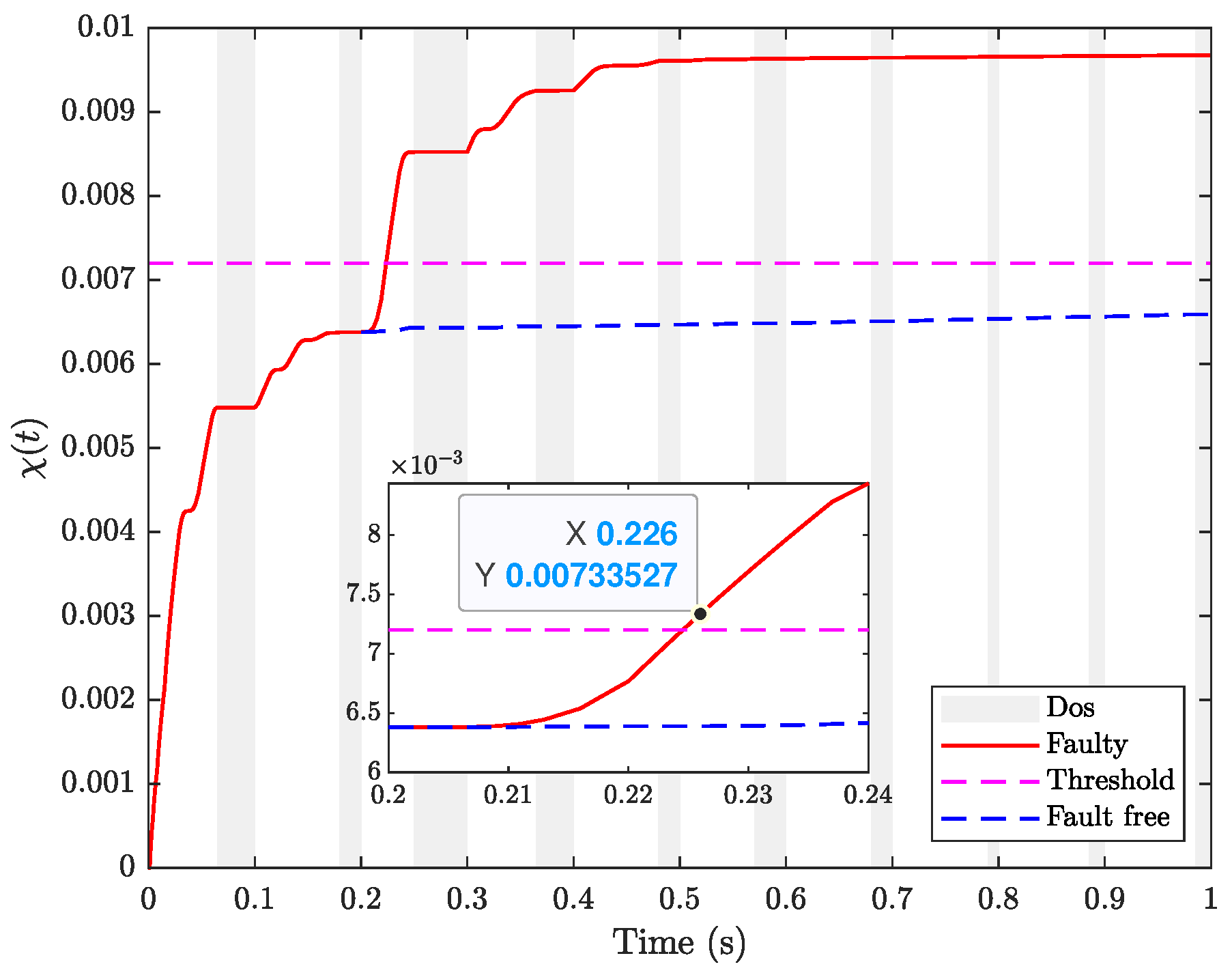
From Figure 5, it is observed that the general FDF detects the fault until s, which is slower than the proposed method for the fault detection in Figure 4 ( s). The proposed FDF method in this study is designed for the fault occurring within a specified frequency band, thereby exhibiting less conservatism compared to general methods designed to detect faults across the entire frequency.
5. Conclusions
A resilient event-based FDF for DC microgrids against DoS attacks has been designed in this paper, where the actuator fault is assumed to occur in a finite-frequency domain, reducing more conservatism in the FDF design. The T-S fuzzy model is used to handle nonlinear CPLs in DC microgrids, and a novel integrated ETM is proposed to further decrease the unnecessary triggering events compared to the traditional ETM. By constructing the switched residual system based on fuzzy rules, sufficient conditions of exponential stability are obtained, along with the attenuation bound and sensitive condition. The simulation results demonstrate the FDF’s ability to rapidly detect finite-frequency faults, even in the presence of a DoS attack. Notably, its superior performance compared to the conventional method underscores the effectiveness of the proposed approach. For future research, fault detection against hybrid attacks for DC microgrids requires deeper investigation.
References yes
Author Contributions
Conceptualization, methodology, writing—original draft preparation, B.M.; software, B.M. and Q.L.; validation, B.M. and Z.G.; formal analysis, Z.G.; investigation, Q.L.; resources, Q.L.; writing—review and editing, B.M. All authors have read and agreed to the published version of the manuscript.
Funding
This research was funded by a project grant from the Natural Science Foundation of Jiangsu Province of China under Grant BK20231288.
Institutional Review Board Statement
Not applicable.
Informed Consent Statement
Not applicable.
Data Availability Statement
The data presented in this study are available on request from the corresponding author.
Conflicts of Interest
The authors declare no conflicts of interest.
References
- Hou, N.; Ding, L.; Gunawardena, P.; Wang, T.; Zhang, Y.; Li, Y.W. A Partial Power Processing Structure Embedding Renewable Energy Source and Energy Storage Element for Islanded DC Microgrid. IEEE Trans. Power Electron. 2022, 38, 4027–4039. [Google Scholar] [CrossRef]
- Al-Ismail, F.S. DC microgrid planning, operation, and control: A comprehensive review. IEEE Access 2021, 9, 36154–36172. [Google Scholar] [CrossRef]
- Dragičević, T.; Lu, X.; Vasquez, J.C.; Guerrero, J.M. DC microgrids—Part I: A review of control strategies and stabilization techniques. IEEE Trans. Power Electron. 2015, 31, 4876–4891. [Google Scholar]
- Liu, J.; Lu, X.; Wang, J. Resilience analysis of DC microgrids under denial of service threats. IEEE Trans. Power Syst. 2019, 34, 3199–3208. [Google Scholar] [CrossRef]
- Herrera, L.; Zhang, W.; Wang, J. Stability analysis and controller design of DC microgrids with constant power loads. IEEE Trans. Smart Grid 2015, 8, 881–888. [Google Scholar]
- Gu, Z.; Fan, Y.; Sun, X.; Xie, X.; Ahn, C.K. Event-based two-step transmission mechanism for the stabilization of networked T-S fuzzy systems with random uncertainties. IEEE Trans. Cybern. 2023, 54, 1283–1293. [Google Scholar] [CrossRef] [PubMed]
- Zhang, J.; Li, S.; Xiang, Z. Adaptive fuzzy output feedback event-triggered control for a class of switched nonlinear systems with sensor failures. IEEE Trans. Circuits Syst. I Regul. Pap. 2020, 67, 5336–5346. [Google Scholar] [CrossRef]
- Chen, H.; Zong, G.; Zhao, X.; Gao, F.; Shi, K. Secure filter design of fuzzy switched CPSs with mismatched modes and application: A multidomain event-triggered strategy. IEEE Trans. Ind. Inform. 2023, 19, 10034–10044. [Google Scholar] [CrossRef]
- Sun, P.; Song, X.; Song, S.; Stojanovic, V. Composite adaptive finite-time fuzzy control for switched nonlinear systems with preassigned performance. Int. J. Adapt. Control Signal Process. 2023, 37, 771–789. [Google Scholar] [CrossRef]
- Yue, S.; Niu, B.; Wang, H.; Zhang, L.; Ahmad, A.M. Hierarchical sliding mode-based adaptive fuzzy control for uncertain switched under-actuated nonlinear systems with input saturation and dead-zone. Robot. Intell. Autom. 2023, 43, 523–536. [Google Scholar] [CrossRef]
- He, H.; Qi, W.; Yan, H.; Cheng, J.; Shi, K. Adaptive fuzzy resilient control for switched systems with state constraints under deception attacks. Inf. Sci. 2023, 621, 596–610. [Google Scholar] [CrossRef]
- He, Y.; Chang, X.H.; Wang, H.; Zhao, X. Command-filtered adaptive fuzzy control for switched MIMO nonlinear systems with unknown dead zones and full state constraints. Int. J. Fuzzy Syst. 2023, 25, 544–560. [Google Scholar] [CrossRef]
- Shen, Z.; Yang, G.H.; Sun, P. Fault detection approach in finite frequency domain based on delay-dependent H-infinity filter. Control Theory Appl. 2012, 29, 940–944. [Google Scholar]
- Long, Y.; Park, J.H.; Ye, D. Finite frequency fault detection for a class of nonhomogeneous Markov jump systems with nonlinearities and sensor failures. Nonlinear Dyn. 2019, 96, 285–299. [Google Scholar] [CrossRef]
- Chibani, A.; Chadli, M.; Ding, S.X.; Braiek, N.B. Design of robust fuzzy fault detection filter for polynomial fuzzy systems with new finite frequency specifications. Automatica 2018, 93, 42–54. [Google Scholar] [CrossRef]
- Zhai, D.; An, L.; Li, J.; Zhang, Q. Fault detection for stochastic parameter-varying Markovian jump systems with application to networked control systems. Appl. Math. Model. 2016, 40, 2368–2383. [Google Scholar] [CrossRef]
- Li, X.J.; Yang, G.H. Fault detection in finite frequency domains for multi-delay uncertain systems with application to ground vehicle. Int. J. Robust Nonlinear Control 2015, 25, 3780–3798. [Google Scholar] [CrossRef]
- Ding, L.; Han, Q.-L.; Wang, L.Y.; Sindi, E. Distributed cooperative optimal control of DC microgrids with communication delays. IEEE Trans. Ind. Inform. 2018, 14, 3924–3935. [Google Scholar] [CrossRef]
- Xing, L.; Xu, Q.; Guo, F.; Wu, Z.G.; Liu, M. Distributed secondary control for DC microgrid with event-triggered signal transmissions. IEEE Trans. Sustain. Energy 2021, 12, 1801–1810. [Google Scholar] [CrossRef]
- Chen, Y.; Lao, K.W.; Qi, D.; Hui, H.; Yang, S.; Yan, Y.; Zheng, Y. Distributed self-triggered control for frequency restoration and active power sharing in islanded microgrids. IEEE Trans. Ind. Inform. 2023, 19, 10635–10646. [Google Scholar] [CrossRef]
- Gu, Z.; Huang, X.; Sun, X.; Xie, X.; Park, J.H. Memory-event-triggered tracking control for intelligent vehicle transportation systems: A leader-following approach. IEEE Trans. Intell. Transp. Syst. 2023, 11, 136590–136599. [Google Scholar] [CrossRef]
- Wang, X.; Sun, J.; Wang, G.; Allgöwer, F.; Chen, J. Data-driven control of distributed event-triggered network systems. IEEE/CAA J. Autom. Sin. 2023, 10, 351–364. [Google Scholar] [CrossRef]
- Hu, S.; Yuan, P.; Yue, D.; Dou, C.; Cheng, Z.; Zhang, Y. Attack-resilient event-triggered controller design of DC microgrids under DoS attacks. IEEE Trans. Circuits Syst. I Regul. Pap. 2019, 67, 699–710. [Google Scholar] [CrossRef]
- Zhang, Y.; Wu, Z.G.; Shi, P.; Huang, T.; Chakrabarti, P. Quantization-Based Event-Triggered Consensus of Multiagent Systems Against Aperiodic DoS Attacks. IEEE Trans. Syst. Man Cybern. Syst. 2023, 53, 3774–3783. [Google Scholar] [CrossRef]
- Gu, Z.; Sun, X.; Lam, H.K.; Yue, D.; Xie, X. Event-based secure control of T–S fuzzy-based 5-DOF active semivehicle suspension systems subject to DoS attacks. IEEE Trans. Fuzzy Syst. 2021, 30, 2032–2043. [Google Scholar] [CrossRef]
- Cheng, F.; Liang, H.; Niu, B.; Zhao, N.; Zhao, X. Adaptive neural self-triggered bipartite secure control for nonlinear MASs subject to DoS attacks. Inf. Sci. 2023, 631, 256–270. [Google Scholar] [CrossRef]
- Mardani, M.M.; Vafamand, N.; Khooban, M.H.; Dragičević, T.; Blaabjerg, F. Design of quadratic D-stable fuzzy controller for DC microgrids with multiple CPLs. IEEE Trans. Ind. Electron. 2018, 66, 4805–4812. [Google Scholar] [CrossRef]
- Vafamand, N.; Khooban, M.H.; Dragičević, T.; Blaabjerg, F.; Boudjadar, J. Robust non-fragile fuzzy control of uncertain DC microgrids feeding constant power loads. IEEE Trans. Power Electron. 2019, 34, 11300–11308. [Google Scholar] [CrossRef]
- Zhu, Q.; Jiang, S.; Pan, F. Adaptive event-triggered fault detection for nonlinear networked systems in finite-frequency domain under stochastic cyber-attacks. Int. J. Adapt. Control Signal Process. 2022, 36, 1537–1561. [Google Scholar] [CrossRef]
- Liu, J.; Yin, T.; Cao, J.; Yue, D.; Karimi, H.R. Security control for T–S fuzzy systems with adaptive event-triggered mechanism and multiple cyber-attacks. IEEE Trans. Syst. Man Cybern. Syst. 2020, 51, 6544–6554. [Google Scholar] [CrossRef]
- Hu, S.; Yue, D.; Xie, X.; Chen, X.; Yin, X. Resilient event-triggered controller synthesis of networked control systems under periodic DoS jamming attacks. IEEE Trans. Cybern. 2018, 49, 4271–4281. [Google Scholar] [CrossRef] [PubMed]
- Wang, X.; Fei, Z.; Gao, H.; Yu, J. Integral-based event-triggered fault detection filter design for unmanned surface vehicles. IEEE Trans. Ind. Inform. 2019, 15, 5626–5636. [Google Scholar] [CrossRef]
- Yue, D.; Tian, E.; Han, Q.L. A delay system method for designing event-triggered controllers of networked control systems. IEEE Trans. Autom. Control 2012, 58, 475–481. [Google Scholar] [CrossRef]
- Heemels, W.H.; Donkers, M.; Teel, A.R. Periodic event-triggered control for linear systems. IEEE Trans. Autom. Control 2012, 58, 847–861. [Google Scholar] [CrossRef]
- Ma, Y.; Tang, W.; Sun, X. Integral-Based Event-Triggered Fault Estimation and Accommodation for Aeroengine Sensor. IEEE Trans. Instrum. Meas. 2023, 72, 3001409. [Google Scholar] [CrossRef]
- Zhou, K.; Doyle, J.C. Essentials of Robust Control; Prentice Hall: Upper Saddle River, NJ, USA, 1998; Volume 104. [Google Scholar]
- Fei, Z.; Wang, X.; Wang, Z. Event-based fault detection for unmanned surface vehicles subject to denial-of-service attacks. IEEE Trans. Syst. Man Cybern. Syst. 2021, 52, 3326–3336. [Google Scholar] [CrossRef]
Figure 1.
Circuit diagram of DC microgrids.
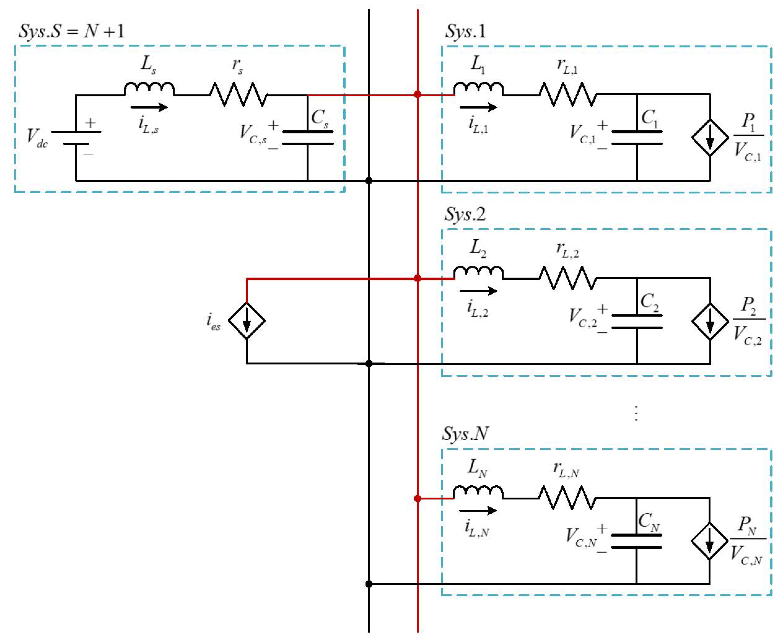
Figure 2.
Impacts of on the system output and the residual signal .

Figure 3.
Release instants under different triggering mechanisms.

Figure 4.
Fault detection performance under different triggering mechanisms.

Figure 5.
Fault detection performance using method.

Table 1.
The DRR under differents ETMs.
| Cases | Traditional ETM | Our Integrated ETM |
|---|---|---|
| Total sampling | 1000 | 1000 |
| Total releasing | 297 | 144 |
| DRR | 29.7% | 14.4% |
Disclaimer/Publisher’s Note: The statements, opinions and data contained in all publications are solely those of the individual author(s) and contributor(s) and not of MDPI and/or the editor(s). MDPI and/or the editor(s) disclaim responsibility for any injury to people or property resulting from any ideas, methods, instructions or products referred to in the content. |
© 2024 by the authors. Licensee MDPI, Basel, Switzerland. This article is an open access article distributed under the terms and conditions of the Creative Commons Attribution (CC BY) license (https://creativecommons.org/licenses/by/4.0/).
Share and Cite
MDPI and ACS Style
Ma, B.; Lu, Q.; Gu, Z. Resilient Event-Based Fuzzy Fault Detection for DC Microgrids in Finite-Frequency Domain against DoS Attacks. Sensors 2024, 24, 2677. https://doi.org/10.3390/s24092677
AMA Style
Ma B, Lu Q, Gu Z. Resilient Event-Based Fuzzy Fault Detection for DC Microgrids in Finite-Frequency Domain against DoS Attacks. Sensors. 2024; 24(9):2677. https://doi.org/10.3390/s24092677
Chicago/Turabian StyleMa, Bowen, Qing Lu, and Zhou Gu. 2024. "Resilient Event-Based Fuzzy Fault Detection for DC Microgrids in Finite-Frequency Domain against DoS Attacks" Sensors 24, no. 9: 2677. https://doi.org/10.3390/s24092677
Note that from the first issue of 2016, this journal uses article numbers instead of page numbers. See further details here.