1. Introduction
Fishing is an important industry in Morocco, and the waters off the coast of this country are rich in fish. The fish catch includes sardines, tuna, mackerel, anchovies and shellfish. Sardines represent 80 % of all fish caught each year, and, according to the statistics of the National Office for Fishing (2004), 42.14 % of all fish exported. Much of the catch is processed in Morocco –fresh, frozen or canned– for export. One of the unique characteristics of fish as food is that it is a highly perishable commodity [
1]. In fact, the time spent after its catch and its temperature ‘history’ are very often the key factors determining the final quality characteristics of fish or fish products. Consequently, there is a need for a technique to monitor freshness and quality of fish (Sardine). As an important indicator of fish freshness, analysis of odours has traditionally been performed either by sensory panels or by gas chromatography coupled to mass spectroscopy, which are time consuming and costly [
2,
3]. To this end, the electronic nose has proven to be a rapid and non-destructive method for evaluating volatile compounds, which are derived from spoilage odours in fish [
4,
5].
The two main components of an electronic nose are the sensing system and the automated pattern recognition system. The sensing system can be an array of different sensing elements (e.g. gas sensors), where either each element measures a different property of the sensed odour or, more often, the sensors respond to a complex odour with overlapped sensitivity, which results in the sensor array producing a characteristic signature or pattern. Thus, presenting the odour of many samples of sardines at different times of cold storage to the sensor array will result in a database of signatures being built up [
6]. This database of signatures will be then used to train the pattern recognition system. The goal of this training process is to configure the recognition system to produce unique classifications of each sample of sardines, so that an automated identification can be implemented. The pattern recognition system comprises the feature extraction step, which extracts useful information from the sensor responses and the pattern recognition algorithm. In supervised pattern recognition, input patterns are learned and associated with an odour class. In an unsupervised pattern recognition technique, the multidimensional configuration space from the pre-processor is converted into a feature space. The unknown sardine sample is identified by comparison to a knowledge base, from a previous learning scheme. The pattern recognition algorithms have become a critical component in the successful implementation of gas sensor arrays and electronic noses. Among many pattern recognition techniques, we are interested in those based on artificial neural networks (ANN).
Similar to the brain of mammals, an ANN is composed of neurones, regarded as the processing units, and the massive interconnection among them. ANN have the unique ability to learn from examples and to generalise, i.e., to produce reasonable outputs for new inputs not encountered during a learning process [
7]. Electronic noses that incorporate ANNs have been demonstrated in various applications. Many ANN configurations and training algorithms have been used to build up electronic noses [
8] including probabilistic neural networks (PNN), backpropagation-trained feed-forward networks, fuzzy ARTMAP neural networks (FANN), Kohonen's self-organising maps (SOMs), learning vector quantization (LVQs), Boltzmann machines, Hopfield networks and support vector machines (SVM).
In this study, we introduce an electronic nose system capable of discriminating sardine samples according to the number of days spent under cold storage. The system is composed of an array of six commercially available metal oxide semiconductor gas sensors and an artificial neural network as the pattern recognition algorithm. Three different neural networks (PNN; FANN and SVM) have been evaluated in the classification of data obtained with our electronic nose measurement system.
2. Experimental
2.1. Electronic nose set-up
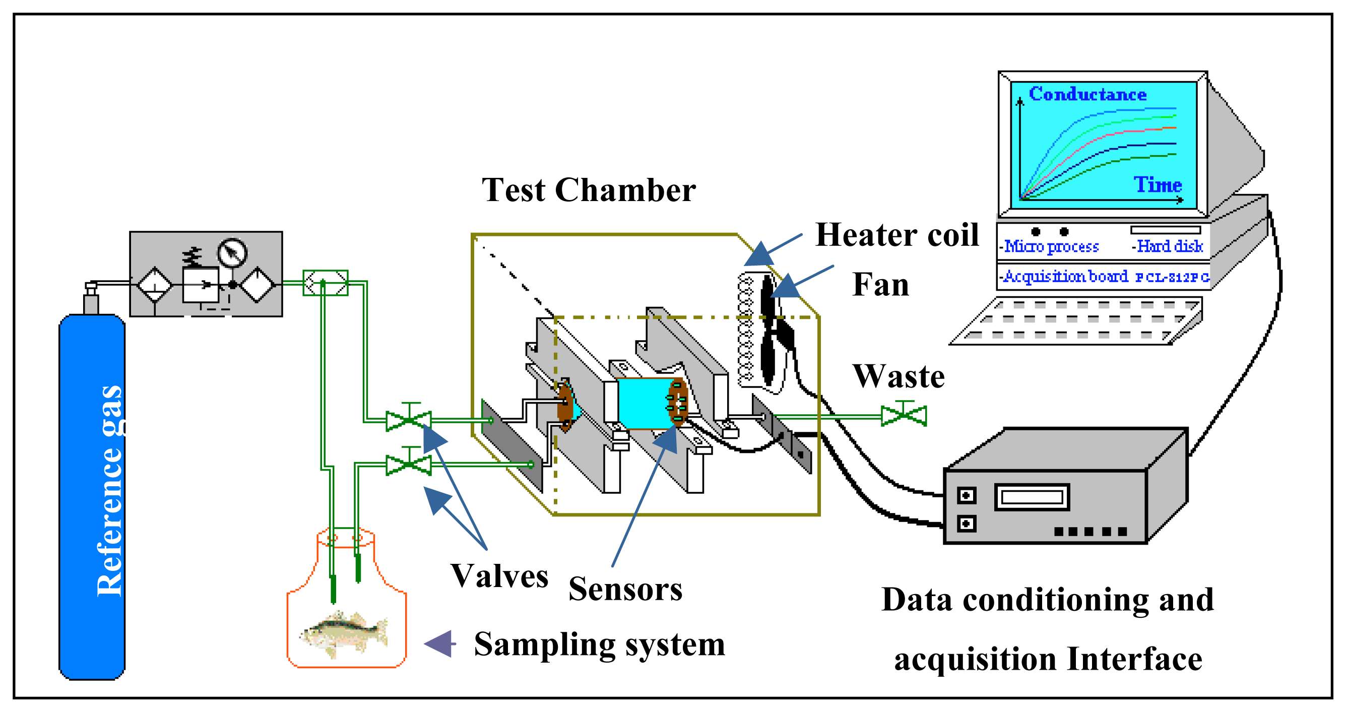
The electronic nose system was designed to be able to control the quality of sardine samples during cold storage (up to 15 days). Three main parts compose this system: The sampling system, the sensor chamber and the data acquisition system. An overall view of the system is shown in
figure 1. The sampling system consists of a dynamic headspace sampling. The sensor array comprised six metal oxide gas sensors (TGS type from Figaro Inc.), a capacitive humidity sensor PHILIPS H1 from Philips and a temperature sensor LM35DZ from National Semiconductor. The identification codes of the Figaro sensors that were used are the following, where the target gases as suggested by the manufacturer are indicated: TGS 823 (Alcohols, Xylene and Toluene), TGS 825 (H
2S), TGS 826 (NH
3), TGS 831 (Chlorofluorocarbons), TGS 832 (Halocarbons) and TGS 882 (Alcohols) [
9].
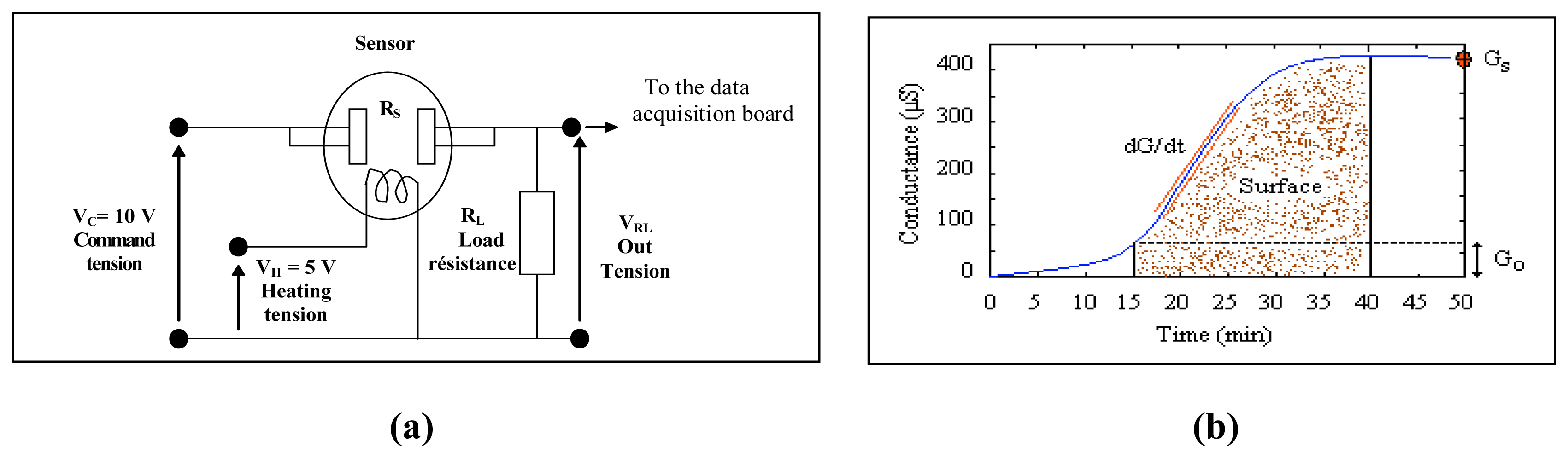
Exposure of a metal oxide semiconductor sensor to an odour (e.g. fish odour) produces a large change in its electrical resistance, the circuit conditioning used to measure the conductance [
10], is shown in
fig.2 (a). The relationship between the sensor resistance and the voltage monitored is expressed by the following equation:
The humidity and temperature sensors are used to monitor the condition of the experiments. The electrical response of the eight sensors was monitored by an acquisition data board (PCL-812) installed in a Compatible Personnel Computer. Pure nitrogen was used as carrier gas. A fan and a heating coil were incorporated into the sensor chamber to keep constant the temperature between 32°C and 33°C.
2.2. Procedure
Sardines used in the experiments have been bought from the local fish market of the city of Meekness (Morocco). The samples were placed in plastic boxes and kept under cold storage at 4 ± 1°C before being analysed. Samples were analysed after 1, 3, 5, 7, 9, 11, 13 and 15 days of cold storage. Ten samples per each storage day were measured, in total 80 sardine samples were analysed. Each sample of sardine was taken from the refrigerator and kept in a sealed sampling vessel 40 min before every experiment. This ensured the homogeneity of sample preparation. For each day of experiment, the sensors were supplied with a 10 V circuit voltage and a 5 V heating voltage 50 minutes before the first measurement in order to stabilise them, and were let powered for all the measurements. The measurement procedure went through the following cycle: first, the carrier gas (nitrogen) was allowed to flow through the sensor chamber for 50 minutes so that the sensors could stabilise their baseline resistance. Afterwards, a valve allowed the nitrogen to flow through the sampling vessel and the sensor chamber for another 50 minutes. The response of the sensors was collected and stored every 1 s. After each measurement, the sensor chamber was opened and cleaned with nitrogen gas to regenerate the sensors' baseline. Right after that, a new measurement with another sardine sample can be started.
2.3. Data acquisition and pre-processing
Data acquisition was controlled from a Compatible PC and the signal of each sensor was recorded as a function of time. The baseline conductance of the gas sensors,
G0i (
t) (
i=1,…,
N), and
N = 6, was defined as the steady-state conductance when pure nitrogen flowed through the sensor chamber. The acquisition started before the nitrogen flow was derived via the sampling vessel. The time evolution of every sensor signal,
GSi (
t), where
GSi (
t) is the conductance of sensor
i while the headspace of a sardine is being sampled, was recorded until all sensors reached the steady state. The response of the sensors was acquired and stored every 1 s for 50 minutes. The associated baselines were then subtracted for each sensor and the difference signal
Gi (
t), was calculated as:
The data set consisted of 80 measurements, which were assigned to 8 different classes according to the number of days the sample had spent under cold storage (1, 3, 5, 7, 9, 11, 13 and 15). Each class comprised a total of 10 measurements (i.e. 10 samples per category were measured). To analyse the response of the electronic nose, four parameters were extracted from each sensor conductance transient
Gi (
t) (
Fig. 2(b)):
- -
The average value of the conductance measured in the interval [0 - 15 min], G0 (0→15min);
- -
The slope of the dynamic conductance calculated from the conductance curve within the interval [15 - 35 min],
;
- -
The area below the conductance curve between 15 and 40 minutes calculated by the trapeze method, (Trapeze area conductance) 15→40min;
- -
The steady-state conductance calculated from the average value of the conductance during the last 5 minutes GS (0→15min).
- -
Given that 4 features were extracted from the response of each sensor and that there were 6 sensors within the array, each measurement was described by 24 features, the data matrix had 80 rows (i.e. measurements) and 24 columns (i.e. variables).
3. Artificial Neural Networks
Neural networks offer a chemometric technique of great potential for the treatment of signals generated by electronic noses based on sensors that can provide non-linear responses. Several types of classifiers based on different ANN-algorithms such as multi-layer perceptron (MLP), radial basis function (RBF), self-organising map (SOM), PNN, FANN and SVM have been used in many electronic nose applications [
11-
15]. The nature of an ANN-algorithm is usually classified as a supervised or unsupervised method.
In a supervised learning ANN method, a set of known odours are systematically introduced to the electronic nose, which then classifies them according to known descriptors or classes held in a knowledge base. Then, in a second stage for identification, an unknown odour is tested against the knowledge base, now containing the learnt relationship, and then the class membership is predicted.
For unsupervised learning, ANN methods learn to separate the different classes from the response vectors without any additional information. In other words, unsupervised methods discriminate between unknown odour vectors without being presented with the corresponding descriptors. These methods are closer to the way that the human olfactory system works. They both use intuitive associations with no, or little, prior knowledge.
In order to evaluate their performance in the classification of sardine samples, three supervised learning approaches (PNN, FANN and SVM) were applied to analyse the data set described above.
3.1. Probabilistic neural network (PNN)
The probabilistic neural network was developed by Donald Specht. This network provides a general solution to pattern classification problems by following an approach developed in statistics called Bayesian classifiers. Bayes' theory, developed in the 1950's, takes into account the relative probability of events and uses a priori information to improve prediction. The probabilistic neural network uses a supervised training set to develop distribution functions within a pattern layer [
8,
16]. The Probabilistic Neural Networks (PNNs) approach combines both Bayes theorem of conditional probability and Parzen's method for estimating the probability density functions of random variables. Unlike other neural network training paradigms, PNNs are characterised by high training speed and their ability to produce confidence levels for their classification decisions. For theoretical background and details of the algorithm, the reader is referred to [
16-
18]. The PNN was first introduced by Specht [
18], who showed how the Bayes–Parzen classifier could be broken up into a large number of simple processes implemented in a multilayer neural network which could be run independently in parallel.
3.2. Fuzzy ARTMAP neural networks (FANN)
The Fuzzy ARTMAP neural network is a supervised pattern recognition method based on fuzzy adaptive resonance theory (ART). It is a promising method since fuzzy ARTMAP is able to carry out on-line learning without forgetting previously learnt patterns (stable learning). It can also recode previously learnt categories (adaptive to changes in the environment) and is self-organising [
19]. In its most general form, Fuzzy ARTMAP includes two fuzzy ART modules (ART
a and ART
b) interconnected by an associative memory and some internal control structures that regulate learning and information flow [
20]. During supervised learning ART
a receives a stream of input patterns {a
M} and ART
b also receives a stream of patterns {b
M}, where b
M is the correct prediction given a
M. When a prediction by ART
a is not confirmed by ART
b, inhibition of the inter-ART associative memory activates a match tracking process. This increases ART
a vigilance by the minimum amount needed for the system either to activate an ART
a category that matches the ART
b category or to learn a new ART
a category.
3.3. Support vector machines (SVM)
In the last decade, a new classification technique called support vector machines (SVM) has been proposed in the broad learning. SVM, which is based on statistical learning theory (SLT), has recently been introduced as a new technique for solving a variety of learning classification and prediction problems [
21,
22]. SVM have been successfully applied to a number of problems ranging from face identification and text categorisation to bioinformatics and data mining.
Support vector machine (SVM) is a statistical classification method proposed by Vapnik in 1995 [
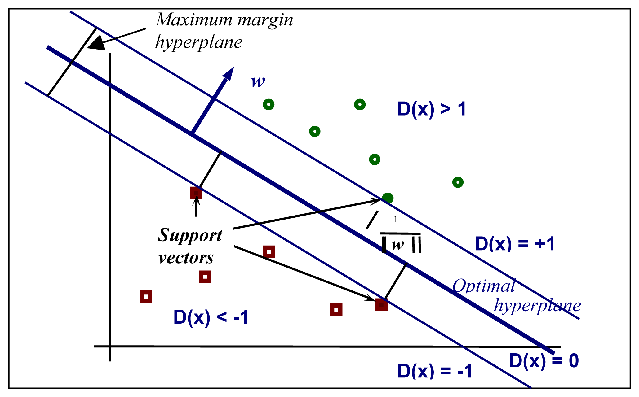
22]. The main idea of SVM is to separate the classes with a particular hyperplane, which maximises a quantity called
margin. The margin is the distance from a hyperplane separating the classes to the nearest point in the dataset (
Fig. 3).
In the separable case, a hyperplane,
ω separates positive and negative samples. Those data
x that satisfy 〈
w, x〉 +
b =0 lie on the hypeplane where
ω is normal to the hyperplane (
ω ∈
Rn and
b ∈
R),
b/‖
ω‖ is the perpendicular distance from the hyperplane to the origin. Samples from positive and negative training samples satisfy:
yi (〈
ω, xi〉+
b) ≥ 1 where
xi ∈
IRn and
yi ∈ {−1,1}. The decision function is defined as:
where
αi are the Lagrange multipliers obtained by solving the optimisation problem [
22].
One class is assigned when the decision function is positive and the other when it is negative. When the classes are non-linearly separable in input space, training patterns are mapped into a higher dimensional space (feature space)
x ∈ ℜ
n → Φ(
x) ∈ ℜ
f, where the problem is linearly separable. By introducing kernel functions,
K, the required scalar products in feature space are calculated directly by computing kernels in input space, which avoids having knowledge about the actual mapping Φ(
x). In this case, the decision function is modified as follows:
The positive value of f(x) is associated with 1 and the negative one with -1.
Support vector machines (SVM) were originally designed for binary classification. Currently there are two types of approaches for multi-class SVM. One is by constructing and combining several binary classifiers “one against one or one against all methods”, while the other is by directly considering all data in one optimisation formulation [
23]. The direct approach constructs a classifier recognising the set of classes: the determination of the hyperplane between these different classes permits to choose a class among the
k when a new input is presented. In order to carry out a comparative study, we have applied the direct approach that is considered a suitable method for practical use. This algorithm is clearly described by J. Weston in [
24]. The kernel function used in this study is polynomial (degree = 3) with an optimal value of the penalty coefficient C = 2
17.
4. Results and discussion
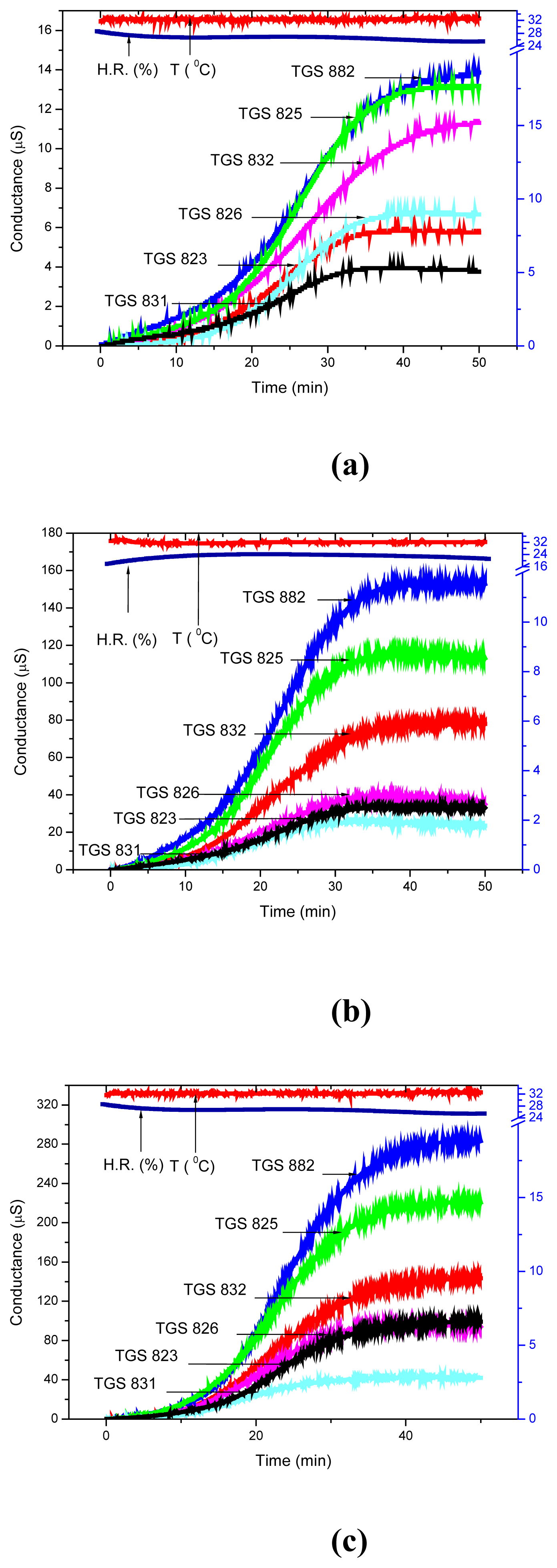
The effect of the number of storage days in a refrigerator,
D, undergone by the sardine samples on the sensor array response was analysed at first. Hence, every two days, a sample of sardine was taken out of the refrigerator and the array response was recorded as function of time,
t, until steady state was reached for every sensor. A plot of the time dependence of
Gi (
t) when the sensors are exposed to a sample of sardine after 3, 5 and 9 days of cold storage is shown in
Fig. 4. It can be shown that the sensor signals reach a plateau and the conductance of the sensors dramatically increases with storage days. This indicates that the concentration of volatile compounds, which characterise the spoilage odour of fish [
6], increases with the number of storage days. We note that all the TGS gas sensors showed reducing gas behaviour: i.e., sensor conductance increased when fish volatiles were sampled.
However, the major problem with sensors used in electronic noses is their response drift [
25]. Sensors can be problematic due to a change of response pattern with time, these drifts must be minimised by measuring dummy samples before the actual samples. The relative humidity changes slightly with time (
Fig. 4) and mainly depends on the number of storage days of the fish, but does not affect the results and the conclusions obtained [
9]. The temperature inside the chamber remains almost constant in every experiment (about 32 °C).
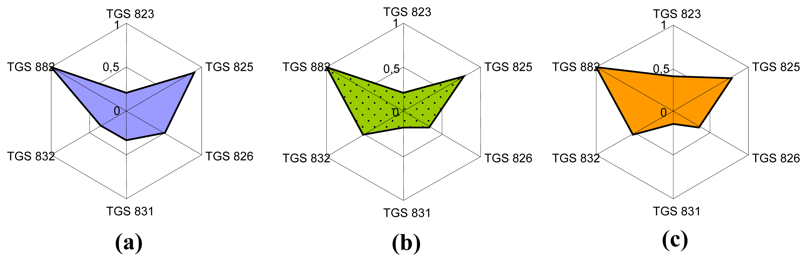
Radar-like plots with unitary radius were performed in order to see whether pattern differences developed between fish samples with different storage days.
Fig. 5 shows a representative case. To construct these plots, the values of
Gi (
t) were divided by the value corresponding to sensor TGS 882, which showed the maximum signal. This helps to easily visualise the differences among typical patterns. The radar plots show at a glance a clear pattern variation between 3 and 5 or 9 days of storage. The shape of the patterns remains very similar for storage days that are previous to a particular day
Dth (day3), referred as the threshold day. It is then possible to differentiate between fish of good (day 1 to day 3) (
Fig. 5(a)) and moderate freshness (day 5 to day 9) (
Fig. 5(b) and (c)) [
26]. It can be seen that each storage day has different pattern. The data associated to the threshold day was always coincident with the expiration day indicated by the sardine seller.
4.2. Data analysis
The data collected with our electronic nose was treated and analysed with three supervised classification methods. These supervised methods were applied with normalised data, for the different classification tasks. To compare the classification accuracy of the three pattern recognition algorithms (PNN, FANN and SVM) used, leave-one-out and
N-fold cross validation techniques were implemented. For the second validation approach, the data set was divided into
5 subsets (
N=5), each subset was made of 16 data vectors. The response patterns constituting the training and testing sets were rotated so that we would have unique training and testing sets in every fold. Response patterns were grouped in 8 categories, which corresponded to 1, 3, 5, 7, 9, 11, 13 and 15 days of storage. While most of the samples belonging to the first four classes could be correctly classified, the success rate in classification decreased noticeably for samples belonging to the other classes. This is true for the 5 different training and validation folds available and for the three different classifiers implemented (
Table 1).
The performance in identification is shown in
Table 2 as a confusion matrix. Rows and columns indicate true and predicted values, respectively. The validation was performed on the whole data set, since the leave-one-out validation technique was used. In the confusion matrix that corresponds to the PNN classifier (
Table 2(a)), errors are quantitatively and qualitatively higher than those of the FANN (
Table 2(b)), and the SVM methods (
Table 2(c)). In particular, when the PNN classifier was used, more samples were wrongly classified and many samples belonging to storage days from 9 to 15 were classified as belonging to class 1 (one day of storage). Besides, the number of classification errors within samples stored from 9 to 15 days is significant, even for fuzzy ARTMAP and SVM based classifiers.
On the other hand, the results reported by El Marrakchi et al. [
26] indicate that sardines have a shelf life of 9 days (if kept under cold storage). According to this, class 5 (day 9), class 6 (day 11), class 7 (day 13) and class 8 (day 15) were grouped together in a new class.
In the second study, the three classifiers were used to sort sardine samples in five classes only (i.e. 1, 3, 5, 7 and 9 or more days of cold storage). Comparing the prediction error of the three different methods, which was estimated using the leave-one-out procedure, it was revealed that the PNN method gave poor classification results with a 35 % error. On the other hand, the fuzzy ARTMAP neural network and SVM performed well with classification errors estimated at 5 % and 3.75 %, respectively. These results are summarised in
Table 3. It is important to note that the proposed method based on SVM gives the best generalisation with a success-rate in classification of 96.25 %. The confusion matrix for the PNN approach is shown in
Table 3(a). Errors are quantitatively higher in this case since 23 samples that had been under storage from 7 to 15 days were classified as fresh sardine samples.
Table 3(b) and Table 3(c) show respectively the confusion matrix for the FANN and SVM approaches. Both methods result in a low number of misclassified samples (4 and 3 respectively). Moreover, we note for the two approaches, that the errors are qualitatively negligible in the sense that errors occur between consecutive categories Furthermore, these two methods are able to correctly separate fresh sardine samples from those that had undergone cold storage.
Table 4 summarizes the results of sardine classification when a 5-fold cross validation procedure was implemented to estimate the success rate of the different classifiers studied. The results show the superior performance of the support vector machine model with a classification success rate of 91.25 % (averaged over the 5 folds), when compared to probabilistic neural network and fuzzy ARTMAP neural network techniques (51.25 % and 88.75 % respectively). These results, although slightly different from those obtained when a leave-one-out cross-validation was used, do not differ in the essential. Namely, SVM, and then FANN are significantly better techniques than the conventional PNN. The SVM method shows improved classification performance, and gives a good estimate of the number of storage days undergone by sardine samples.
5. Conclusions
In this paper, we have demonstrated the feasibility of an electronic nose based on an array of semiconductor gas sensors to detect off-odours from sardines under cold storage. Preliminary results seem very promising for the development of an electronic nose devoted to the monitoring of fish freshness, mainly when a rapid control is needed.
The sensor array coupled with feature extraction and pattern recognition methods can be trained to classify the fish according to the number of days spent under cold storage. In this study, the freshness of sardines has been evaluated with an electronic nose using three pattern recognition methods (PNN, FANN and SVM); the objective being to find the best method able to identify the number of days spent under cold storage with minimal errors. A leave-one-out and an N-fold cross validation techniques have been used in order to obtain a good estimate of the success rate in sardine classification for the different pattern recognition methods studied.
Our results indicate that the performance of SVM was superior to that of PNN and FANN. The superior performance of SVM over PNN or FANN may be due to the following reason: SVM implement the structural risk minimisation principle that minimises an upper bound for the generalisation error rather than minimising the training error.

 ,
, 


