Impact of Altimeter Data Processing on Sea Level Studies

Abstract

This study addresses the impact of satellite altimetry data processing on sea level studies at regional scale, with emphasis on the influence of various geophysical corrections and satellite orbit on the structure of the derived interannual signal and sea level trend. The work focuses on the analysis of TOPEX data for a period of over twelve years, for three regions in the North Atlantic: Tropical (0°≤φ≤25°), Sub-Tropical (25°≤φ≤50°) and Sub-Arctic (50°≤φ≤65°). For this analysis corrected sea level anomalies with respect to a mean sea surface model have been derived from the GDR-Ms provided by AVISO by applying various state-of-the-art models for the geophysical corrections. Results show that sea level trend determined from TOPEX altimetry is dependent on the adopted models for the major geophysical corrections. The main effects come from the sea state bias (SSB), and from the application or not of the inverse barometer (IB) correction. After an appropriate modelling of the TOPEX A/B bias, the two analysed SSB models induce small variations in sea level trend, from 0.0 to 0.2 mm/yr, with a small latitude dependence. The difference in sea level trend determined by a non IB-corrected series and an IB-corrected one has a strong regional dependence with large differences in the shape of the interannual signals and in the derived linear trends. The use of two different drift models for the TOPEX Microwave Radiometer (TMR) has a small but non negligible effect on the North Atlantic sea level trend of about 0.1 mm/yr. The interannual signals of sea level time series derived with the NASA and the CNES orbits respectively, show a small departure in the middle of the series, which has no impact on the derived sea level trend. These results strike the need for a continuous improvement in the modelling of the various effects that influence the altimeter measurement.

1. Introduction

Sea level change has significant environmental, social and economical impacts. The importance of the estimates of the present rate of sea level change, for example for assessment of climate models or for coastal protection design, requires high accuracy and a realistic assessment of the involved uncertainties.

Sea level measurements are available from tide gauges at coastal locations, which measure sea level relative to a vertical reference on land and from satellite missions with radar altimeters. Satellite altimetry provides high quality measurements of absolute sea level, yielding an invaluable dataset for the analysis of sea level temporal and spatial variability. The main advantage of satellite altimetry over tide gauges is the ability to measure absolute sea level, independently of land movements, and the possibility to eliminate mass redistribution signals due to its nearly global spatial coverage.

Since the launch of the European Space Agency (ESA) satellite ERS-1 in 1991 and the joint NASA/CNES mission TOPEX/Poseidon (T/P) in 1992, two main data sets of continuous satellite altimeter measurements became available for sea level studies. The ERS-1 has been continued by ERS-2 in 1995 and Envisat in 2002. In December 2001 the T/P follow-on mission, Jason-1, has been launched, while TOPEX/Poseidon remained fully operational until January 2006, although in a different orbit since August 2002. In spite of the enormous advances in ERS data improvement, particularly in the accuracy of the radial orbit, it is recognised that the TOPEX/Poseidon mission revolutionised sea level research, providing sea surface height (SSH) measurements with an unprecedented accuracy, overall better than 5 cm for a single pass and better than 2 cm at the global scale, [1]. This improved performance with respect to the ERS missions is mainly due to the higher orbital accuracy and better modelling of the ionospheric correction from the dual-frequency measurements.

Compared to tide gauge measurements satellite altimetry has the advantage of providing nearly global and repetitive measurements of the sea surface height relative to a well defined geocentric reference system. The ESA missions cover the ocean every 35 days (except for the periods corresponding to ERS-1 ice and geodetic phases) within the latitude band -81°.5 ≤ φ ≤ 81°.5; T/P and Jason-1 cover the ocean approximately every 10 days within the latitude band -66° ≤ φ ≤ 66°.

While tide gauge and satellite altimetry are in essence independent data sets, the calibration of altimeter data using tide gauge measurements has helped to discover various problems in the measurements, both of instrumental and processing nature. As a consequence, the various altimeter data sets, including T/P, have undergone a continuous improvement over time. According to [2], with the current set of corrections to T/P data, the tide gauge calibration for T/P is nearly “flat”, and it is no longer considered necessary to apply any tide gauge calibration to altimeter data for sea level studies.

The first estimates of sea level trends using satellite altimetry were made using data from the Seasat and Geosat missions, [3,4]. The use of ERS data for studies of global sea level change was discussed for example by [5-7]. Recent studies of global sea level change use the high quality T/P data or merged multi-mission altimetry data, for example, [8-11] and [2]. A review study on sea level change, its observations and causes is presented in [12]. Regional estimates of sea level change are also crucial to understand the factors driving sea level at the basin scale, [13-17], spatial effects and the relation between meteorological and oceanographic factors. They also give insight into regional dependences of instrument behaviour and geophysical corrections.

The determination of sea level variability from satellite altimetry is influenced by many factors. Amongst the most important are sensor characteristics and long-term stability, and the methods used in the altimeter data processing. The latter can be divided in two major steps: the computation of corrected along track sea level anomalies (SLA) and the estimation methodology used to model sea level variation.

This study focuses on the impact of satellite altimeter data processing on sea level studies with emphasis on the influence of various geophysical corrections and the orbit field in the structure of the derived interannual signal and sea level trend, including regional dependencies.

Measurement of sea surface heights with high precision requires precise orbit determination of the spacecraft and the application of accurate geophysical corrections to the raw range estimate from the travel time of the altimeter pulse, accounting for the interactions of the altimeter signal with the atmosphere and the sea surface. The sea surface height error budget for the TOPEX altimeter is summarised in [1] and [18].

Differences in the methodology for processing altimetry data and in the corrections applied are of secondary concern for many applications using altimetry data, but are crucial for sea level change monitoring, since even small differences in the models used or processing approaches can seriously impact the sea level change estimates and corresponding uncertainties. In particular, the inverse barometer (IB) correction and the sea state bias (SSB) correction are major potential error sources in altimetry measurements. SSB errors may be as large as 5 cm in the absolute SSH and between 1 and 2 cm in the time varying altimeter signal [19]. Errors in the IB correction due only to the dynamic sea surface response to atmospheric forcing are estimated to be on the order of 10% of the correction, [20].

Due to the potential impact of the altimetry data processing on the resulting sea level change estimates, it would be expected that sea level change studies would include a detailed description of the data used, of the geophysical and instrumental corrections applied and of eventual bias and drift corrections. However some sea level change analysis, particularly regional studies, fail to provide such a description of the altimetry data, for example, [21,22], and only a few discuss the uncertainties and impacts on the results, e.g. [6] and [8].

The knowledge of the influence of each geophysical correction on the altimeter measurement is fundamental for sea level studies; the most important impacts are driven by corrections which will induce drifts or long period variations. Therefore this study concentrates on the analysis of the effect on sea level trend of three major geophysical corrections: the wet tropospheric correction, the sea state bias and the inverse barometer effect. The last two are still the main error sources in satellite altimetry. In addition, the influence of the orbit field on sea level variation is also investigated.

2. Study area and data used

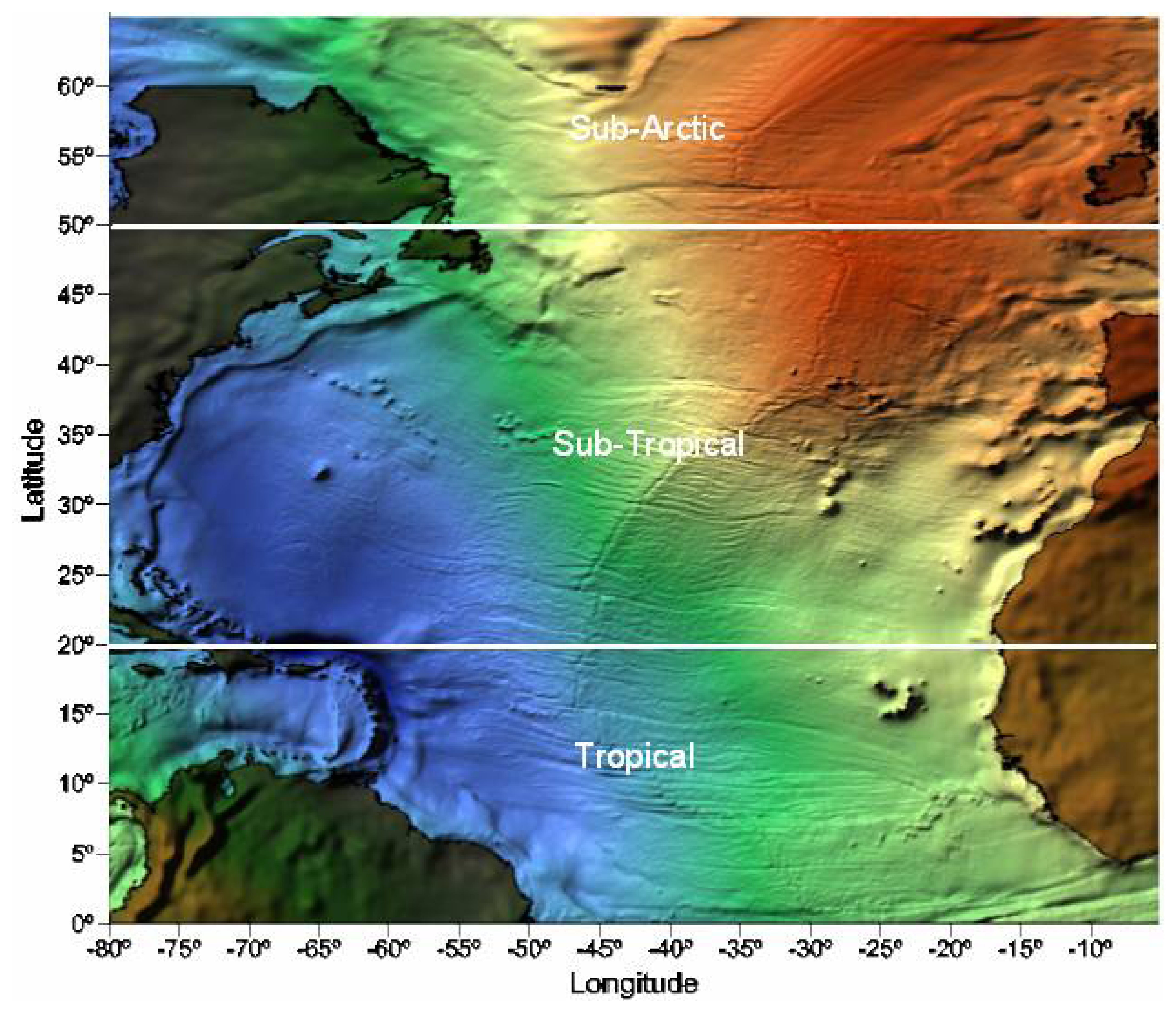
This study focuses on the analysis of sea level change in the North Atlantic for the latitude range 0°-65°N and longitude range 80°W-7°W from TOPEX/Poseidon data (Figure 1). For the purpose of studying regional variations, within the above region three sub-regions were considered: Tropical - T (0°≤φ≤25°), Sub-Tropical – ST (25°≤φ≤50°) and Sub-Arctic – SA (50°≤φ≤65°).

The choice of these three regions is not accidental. Previous studies have shown that these regions possess distinct characteristics in terms of sea level variability [23]. Although the variability inside each region could also be exploited we wanted to keep the number of the analysed time series within a reasonable number and to focus on regional rather than local dependencies.

For T/P data the base products available to users are the Geophysical Data Records (GDR) provided by the Archivage, Validation et Interprétation des données des Satellites Océanographiques (AVISO) or the Physical Oceanography Distributed Active Archive Center (PO.DAAC). There are several versions of the GDR products and it was found that the PO.DAAC products do not exactly mirror the corresponding AVISO products. The altimeter data used in this study are the “Merged Geophysical Data Records” (GDR-Ms) provided by AVISO between October 1992 and February 2005 (Cycles 1 to 460), covering a period of over 12 years. The description of these data can be found in [24].

The decision to use data only from the T/P mission aims to remove effects of possible bias and drifts between data sets of different satellites, which also have an impact on sea level variation. With more than twelve years of operation T/P represents the reference altimeter mission with the longest and most accurate records.

The inclusion of Poseidon data would introduce additional variability related with the bias between the two instruments, their different sea state bias effect and ionospheric corrections (dual-frequency for TOPEX versus DORIS for Poseidon). The number of full Poseidon cycles for this period, which have not been used is 30 (cycles 20, 31, 41, 55, 65, 79, 91, 97, 103, 114, 126, 138, 150, 162, 174, 180, 186, 197, 209, 216, 224, 234, 243, 256, 266, 278, 289, 299, 307, 361). There are also a number of cycles with mixed TOPEX and Poseidon data. Apart from cycles 3, 4, 5, 6, 8, 9, 11, 12, 13, 14, 15, 16, all at the beginning of the mission, for which the percentage of Poseidon measurements in the study region ranges from 10% to 22%, a number of additional 23 cycles were also found to have portions of passes with Poseidon data. However these were only a few measurements, with an average of 0.5% and a maximum of 2%. Even considering this small percentage, these Poseidon measurements were discarded.

During the analysed period the T/P mission experienced two major changes, [25]: in January 1999, at the beginning of cycle 236, the TOPEX altimeter Side-A instrument was replaced by TOPEX Side-B; in August/September 2002 a manoeuvre sequence was conducted (from cycles 365 to 368) to move T/P to a new orbit with tracks half way displaced with respect to the previous ones. The T/P follow-on mission Jason-1 was maintained in the previous T/P orbit. Therefore, during the remaining of the T/P mission the two satellites provided a global coverage of the ocean within the observed latitude bands with twice the spatial resolution of each single mission.

3. Data Processing

3.1. Computation of along-track sea level anomalies

From the raw altimeter measurement until the corrected SSH above a reference ellipsoid or the corresponding sea level anomaly (SLA) with respect to a known mean sea surface (MSS), the most common variable used in sea level studies, a number of corrections have to be applied to data, to account for the interactions with the atmosphere and with the sea surface.

The corrected sea surface height is computed as follows:

$$\mathit{\text{SSH}}=r-\mathit{(}h+\mathit{\text{gcor}}\mathit{)}$$

(1)

where h is the altimeter range corrected for instrumental effects, r is the satellite height above the TOPEX reference ellipsoid and gcor includes all geophysical corrections.

Using the NASA JGM3 orbit, [24] and the set of geophysical corrections summarised in

Table 1. Geophysical corrections and models used in the processing of TOPEX altimeter data (DataSet1).

Corrections/models	T/P
Mean Sea Surface	GSFC00.1, [33]
Orbit	NASA JGM3, [24]
Dry troposphere	ECMWF, [24]
Wet troposphere	Scharroo TMR model (yaw state and drift effect on TMR TBs applied, [26])
Ionosphere	TOPEX: dual-frequency (filtered, [32])
Sea state bias	Chambers model, [27]; additional +2 mm for TOPEX B
Earth tide	Applied, [24]
Ocean tide	NAO99, [31]
Pole tide	Applied, [24]
Inverse barometer	Not Applied

a reference data set, named DataSet1, has been computed. These corrections include: ionospheric correction, dry and wet tropospheric correction (wet_cor), sea state bias (SSB), earth and ocean tides, tidal loading, pole tide. When necessary, the corrections provided on the GDR-Ms were updated to introduce state-of-the-art models as described below.

The cycle dependent drift effect in the TOPEX Microwave Radiometer (TMR) wet tropospheric correction, including the yaw state correction to the TMR measured Brightness Temperatures (TBs), has been modelled according to the Scharroo model, [26].

The SSB correction was derived from the Chambers model [27]; a residual SSB correction of +2 mm was applied to cycles 236 and greater (TOPEX Side-B). This bias is very similar to the +3 mm value referred in [28]. The determination of this bias is explained later in section 4.1.

The TOPEX dual-frequency ionospheric correction has been smoothed using a second order Butterworth filter, [29] with a cut-off period of 20 seconds (λ≈120 km). The result of this filtering is similar to the procedure referred by [30], who used a 20-second averaging window, with the advantage that the effects of discontinuities introduced by data gaps or land regions are minimized.

The ocean tide model used was the NAO99b model, [31], which has been found to give smaller residuals in coastal regions, [32].

In the computation of DataSet1 no inverse barometer correction has been applied.

Sea level anomalies (SLA) have been derived from the corrected sea surface height values by removing the mean sea surface from the GSFC00.1 model, [33]. From the computed SLA data set only the TOPEX measurements for which the rain and the radiometer flag were not set have been selected.

For the purpose of analysing the effect of different models in the geophysical corrections and different orbit solutions other data sets have been derived using the same methodology. In each data set all geophysical corrections applied to DataSet1 have been kept except one, as described below. This information is summarised in

Table 2. Geophysical corrections and models used in the processing of the various TOPEX altimeter data sets. The box corresponding to the correction that has been changed with respect to DataSet1 is shaded.

Data Sets/Corrections	Radiometer Wet troposphere (wet_cor)	Sea state bias (SSB)	Inverse barometer (IB)	Orbit
DataSet1	Scharroo TMR model, [26]	Chambers model, [27]	Not Applied	NASA
DataSet2	Scharroo TMR model, [26]	Labroue model, [34]	Not Applied	NASA
DataSet3	Ruf TMR model,[35]	Chambers model, [27]	Not Applied	NASA
DataSet4	Scharroo TMR model, [26]	Chambers model, [27]	Constant reference atmospheric pressure of 1013.3, [24]	NASA
DataSet5	Scharroo TMR model, [25	Chambers model, [27]	Non-constant reference surface atmospheric pressure. [36]	NASA
DataSet6	Scharroo TMR model, [26]	Chambers model, [27]	Combined-MOG2D model [37]	NASA
DataSet7	Scharroo TMR model, [26]	Chambers model, [27]	Not Applied	CNES

.

• DataSet1 - all corrections according to Table 1.
• DataSet2 - all corrections according to Table 1, except for the SSB where the latest version (Sylvie Labroue, personal communication) of the non-parametric SSB model for TOPEX has been used, [34]. An additional +2 mm SSB correction has been added to all TOPEX B cycles.
• DataSet3 - all corrections according to Table 1, except for the wet tropospheric correction where a slightly modified version of the Ruf model [35] for modelling the TMR drift has been used instead. The modification consisted in the extension of a constant drift rate until cycle 241, followed by a constant drift correction after cycle 241, according to [28]. The parameter ΔL defined in [35] has been replaced by

  $$\{\begin{array}{ll}\mathrm{\Delta }\text{L}=0.0186722*\text{cycle}\_\text{number dB}/\text{cycle}\hfill & \text{if cycle}\_\text{number}<241\hfill \\ \mathrm{\Delta }\text{L}=4.5\text{dB}/\text{cycle}\hfill & \text{if cycle}\_\text{number}\ge 241\hfill \end{array}$$

  (2)

  This correction is similar to the implementation adopted in the generation of the PO.DAAC T/P Sea Surface Height Anomaly product (TPSSHA, PO.DAAC Product:189),[28].
• DataSet4 - all corrections according to Table 1, except for the inverse barometer which has been applied by adopting a model which makes use of a constant reference atmospheric pressure (CRP) of 1013.3 mbar, [24], according to (3).
  $$IB=-9.948*\mathit{(}{P}_{\mathit{\text{atm}}}-1013.3\mathit{)}$$

  (3)

  IB is the inverse barometer correction in mm and P_atm is the surface atmospheric pressure in mbar, computed from the dry tropospheric correction (dry_corr) field provided in the GDR-Ms, using Equation (4), where φ is the geodetic latitude.
  $$P_{\mathit{\text{atm}}}=\frac{\mathit{\text{dry}}\_\mathit{\text{corr}}}{-2.277(1+0.0026cos\left(2\mathrm{\phi }\right))}$$

  (4)
• DataSet5 - all corrections according to Table 1, except for the inverse barometer which has been applied by adopting a model which makes use of a variable reference surface atmospheric pressure (VRP) interpolated from global average values obtained from the Centre National d'Études Spatiales (CNES/CLS), [36], according to equation (5).
  $$IB=-9.948*({\text{P}}_{\mathit{\text{atm}}}-\overline{P})$$

  (5)

  IB is the inverse barometer correction in mm, P_atm is the surface atmospheric pressure in mbar, computed according to (4) and P̅ is the global average pressure interpolated to the time of the measurement from values determined at 6 hour intervals from CNES. According to [36], the values of P̅ have been smoothed using a (2-day)^-1 cut-off frequency.
• DataSet6 - all corrections according to Table 1, except for the inverse barometer which has been applied by adopting a combined model where the low frequencies are taken from the inverse barometer correction according to (5) and the high frequency effects are given by the MOG2D barotropic model [37]. This combined correction has been interpolated from global grids (0.25° × 0.25°) at 6 hour intervals provided by AVISO and it will be referred as “combined-MOG2D IB model”.
• DataSet7 - all corrections according to Table 1, except for the satellite orbit, where the satellite height above ellipsoid from the NASA JGM3 orbit was replaced by the CNES solution [24].

3.2. Determination of interannual variation and sea level trend

For each of the above described data sets, the along track sea level anomalies for each TOPEX cycle have been gridded using a 0.5° spacing. For each non empty 0.5° block the along-track SLA values are replaced by the median value at the centre of the block.

Time series of spatially aggregated sea level anomalies for the Tropical, Sub-Tropical and Sub-Arctic Atlantic regions are obtained through spatial averaging of SLA values for each cycle with equi-area weighting by a cosine function of latitude to account for the relative geographical area represented by each block. As mentioned before, only TOPEX measurements have been used. The 30 full Poseidon cycles were discarded and replaced by interpolated values; missing TOPEX cycles (118, 432, 433) were also replaced by interpolated values from adjacent cycles. Considering the 7 datasets and the three mentioned regions a total number of 21 time series of SLA values were generated. 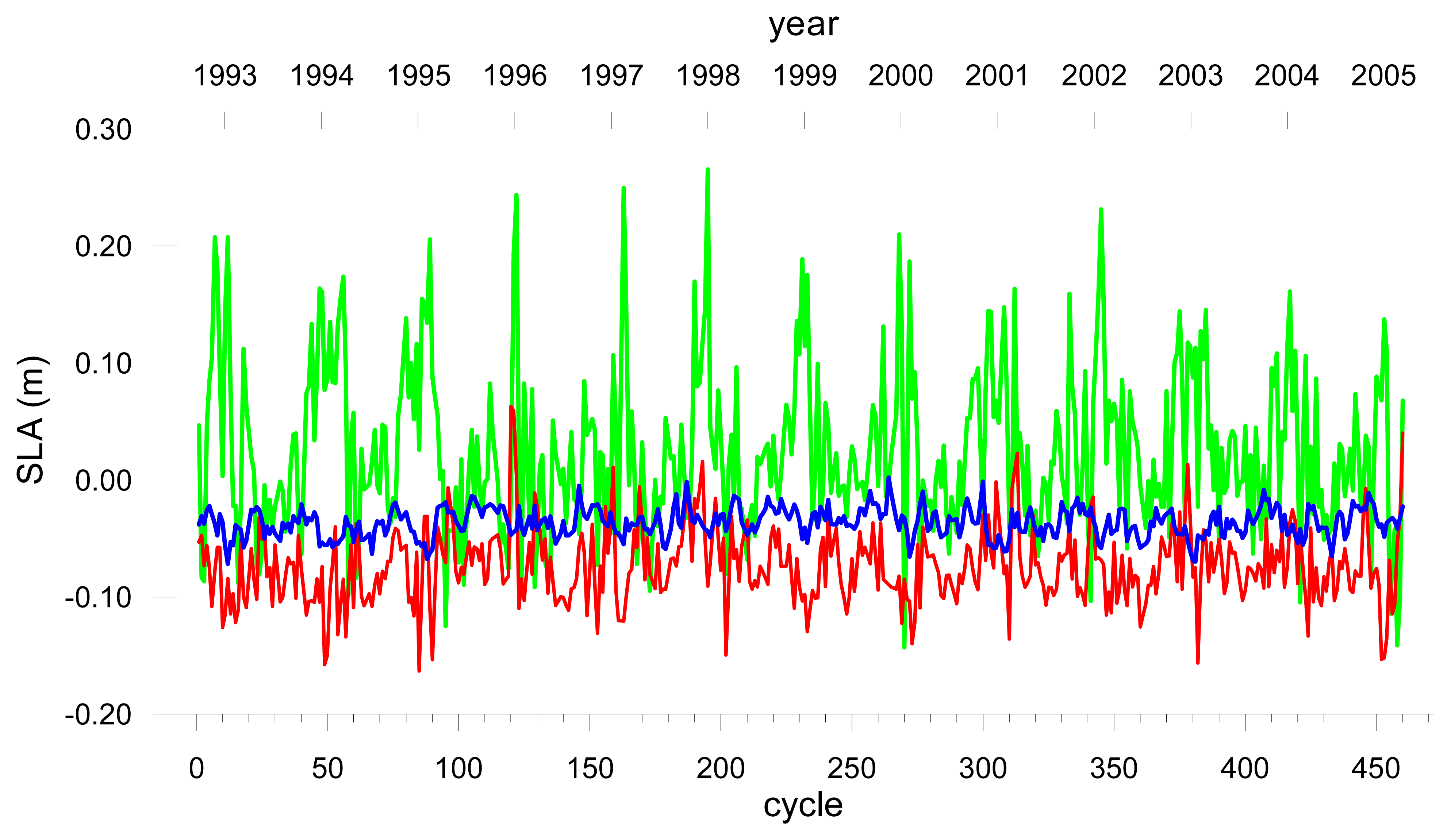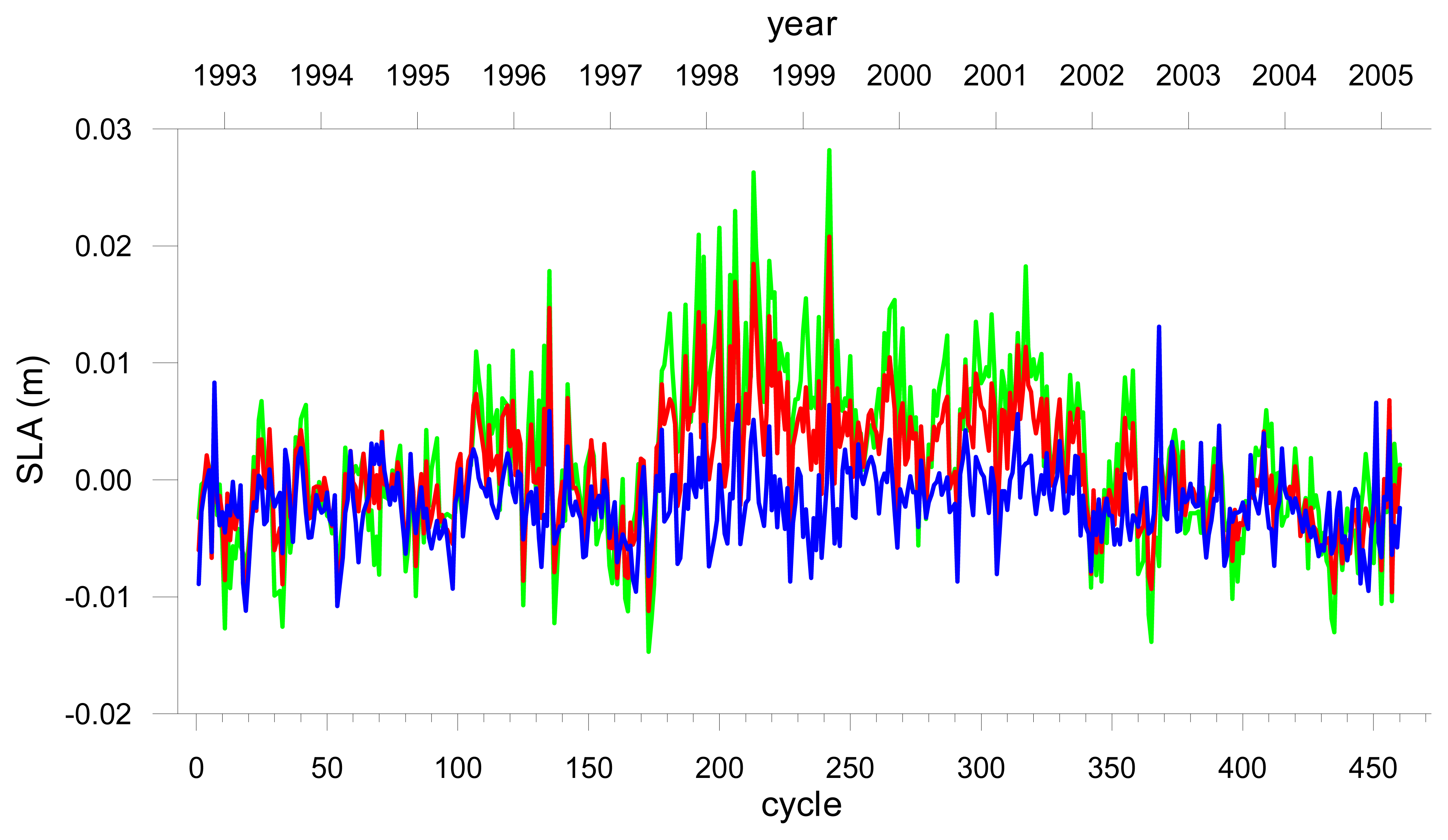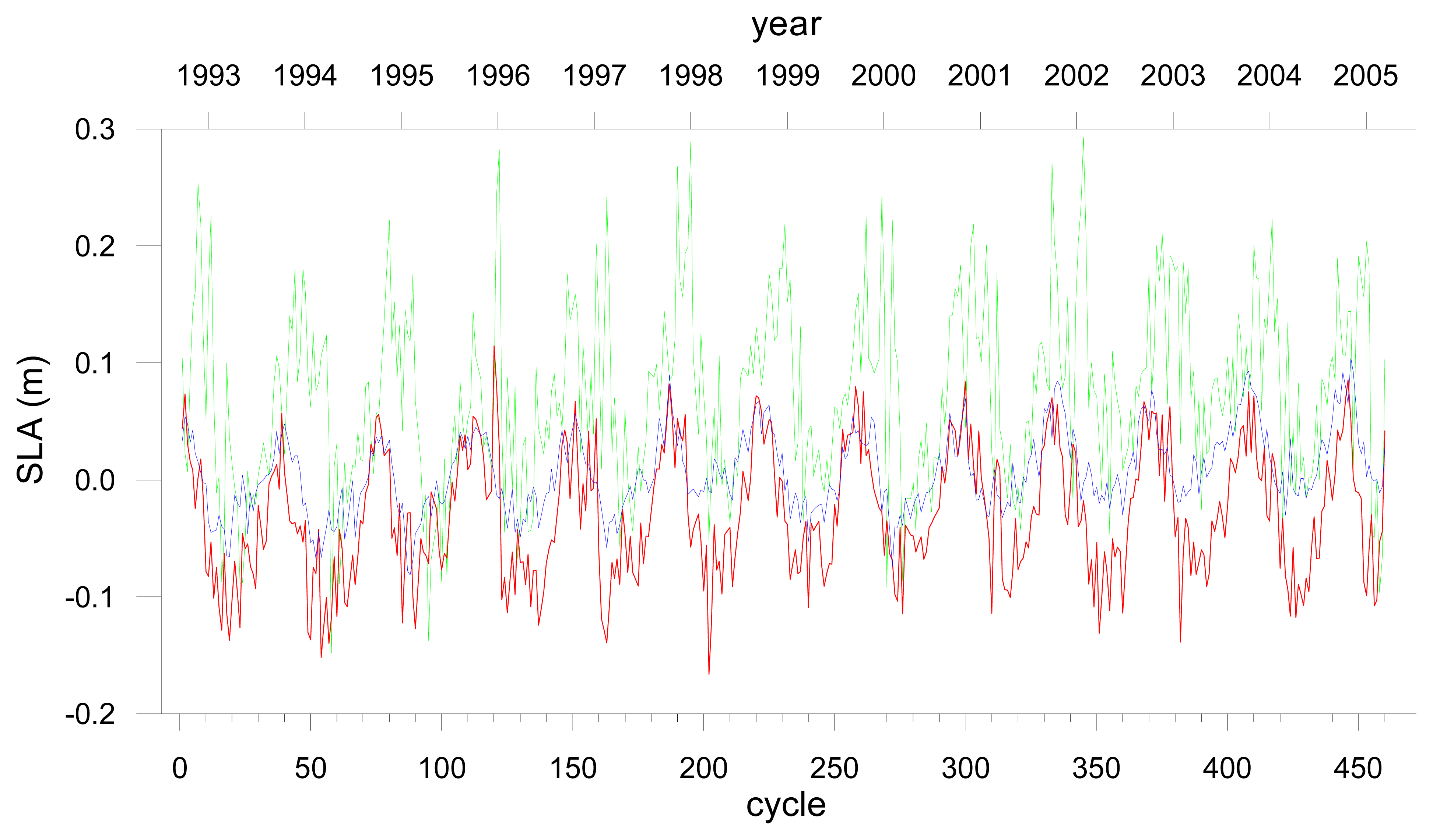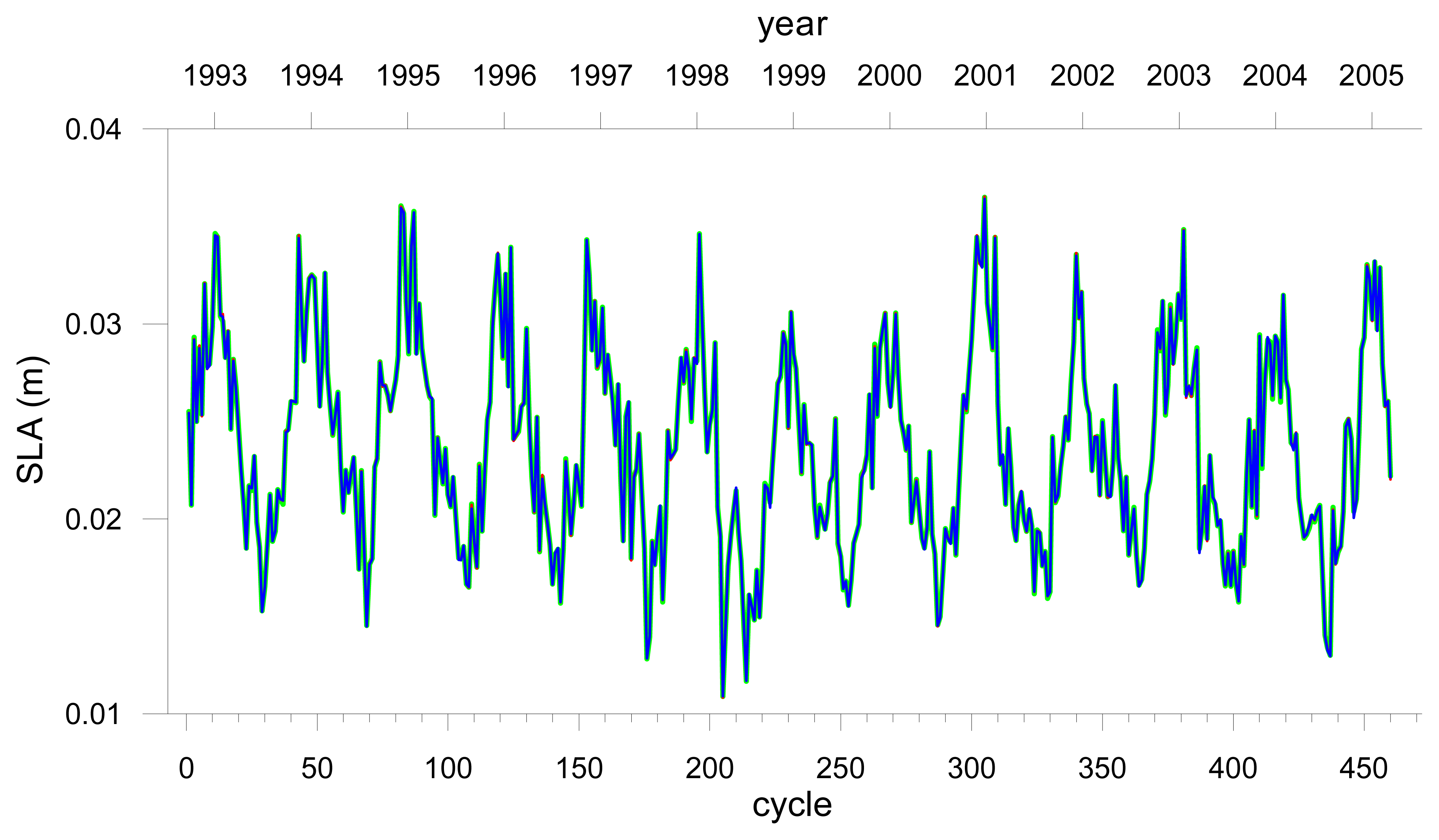Figure 2 shows the sea level anomalies for DataSet1 in each of the three regions.

Flexible and robust non-parametric estimates of sea level inter-annual variability are obtained using STL, acronym for “Seasonal-Trend decomposition based on Loess”, [38]. Details concerning the non-parametric estimate of long-term sea level variability are given in [39]. STL decomposition is carried out for each time series of sea level anomalies using R implementation [40].

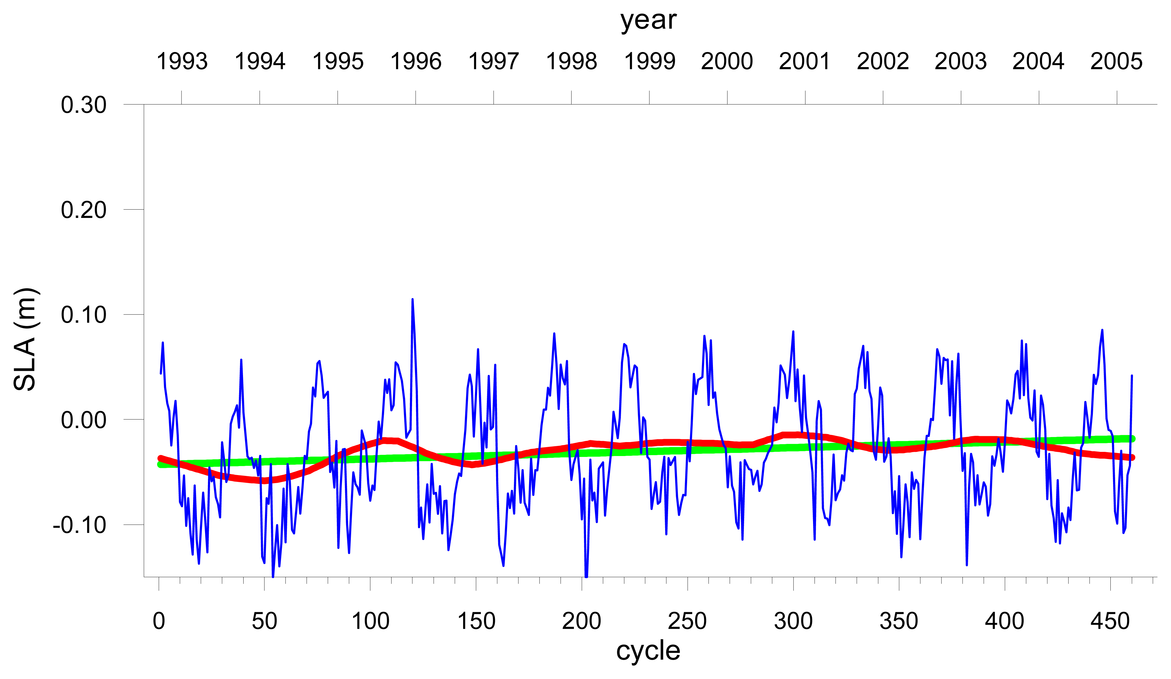
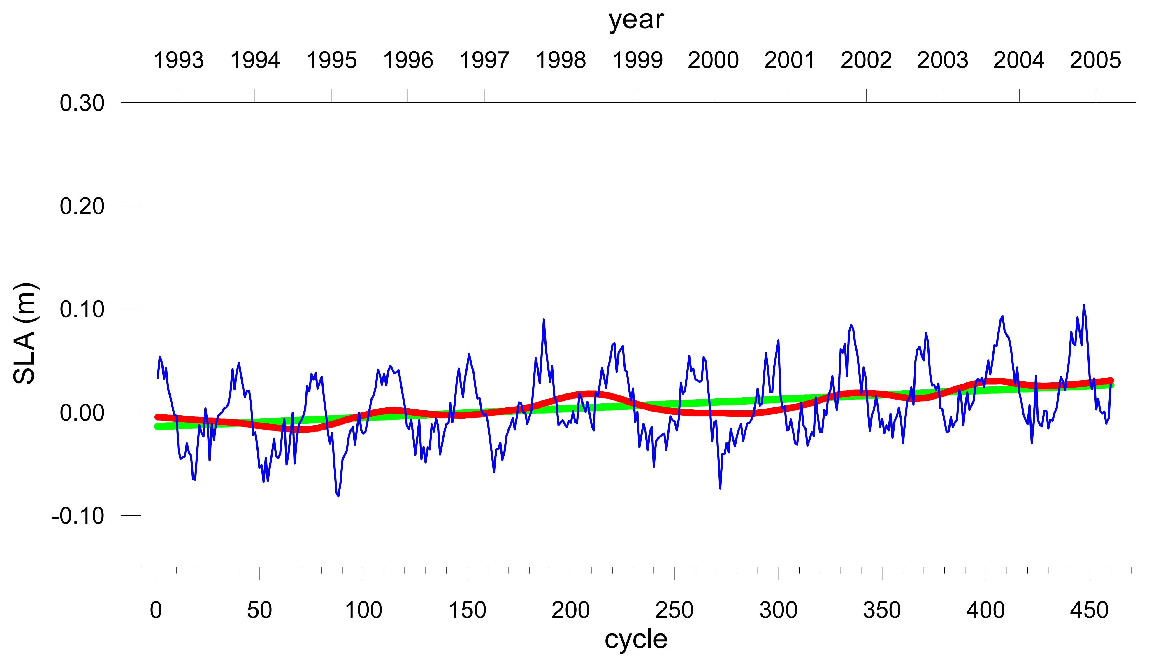
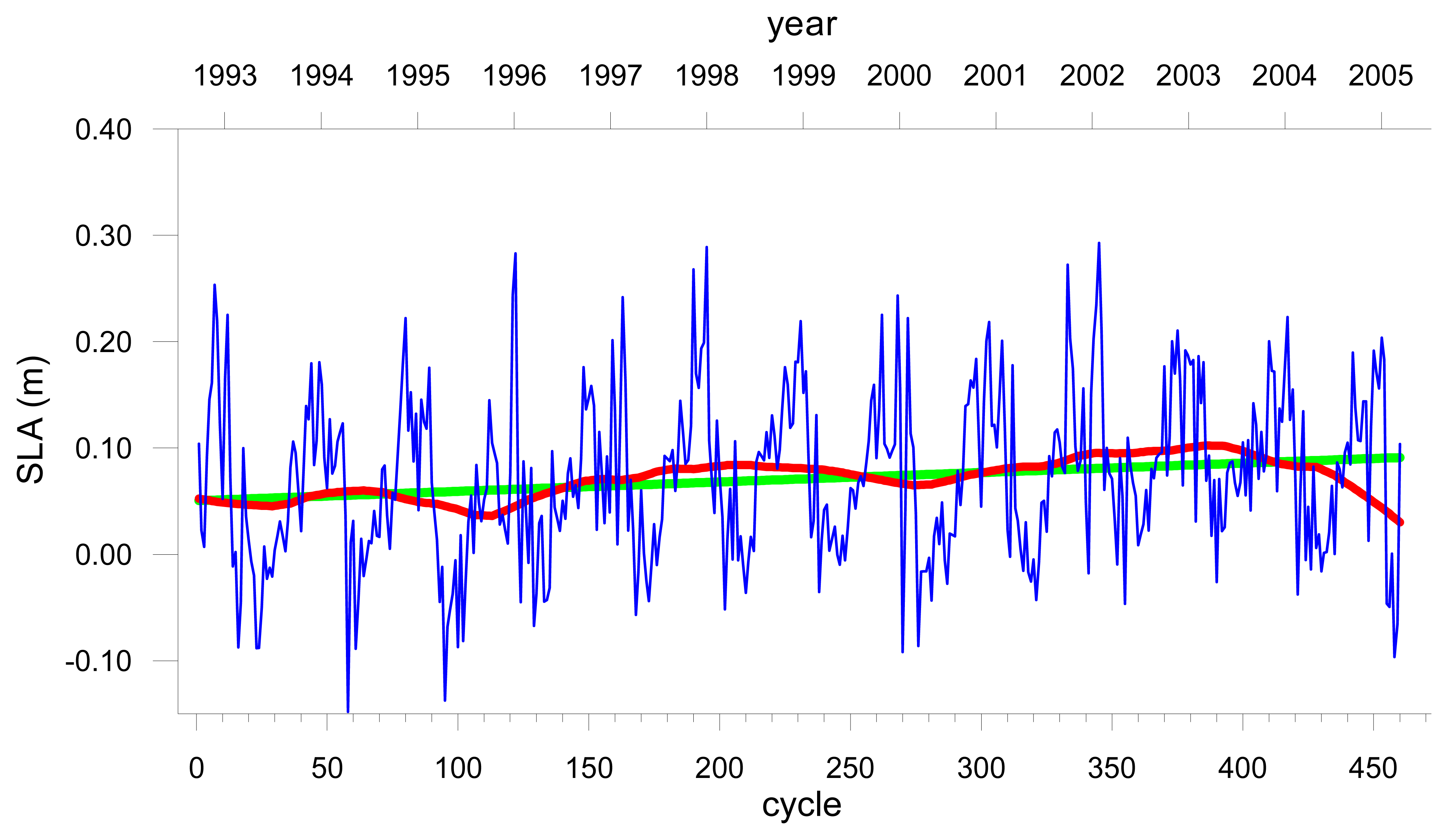
Sea level linear trend is finally estimated for each time series, using an ordinary least squares (OLS) adjustment to each interannual curve, [41]. For DataSet1, Figures 3a, 3b and 3c show the original SLA values, the interannual variations and the linear trend for the T, ST and SA regions respectively.

4. Results and Discussion

The process described in the previous section has been applied to each of the 21 time series. In this section the results obtained for each series are presented and discussed.

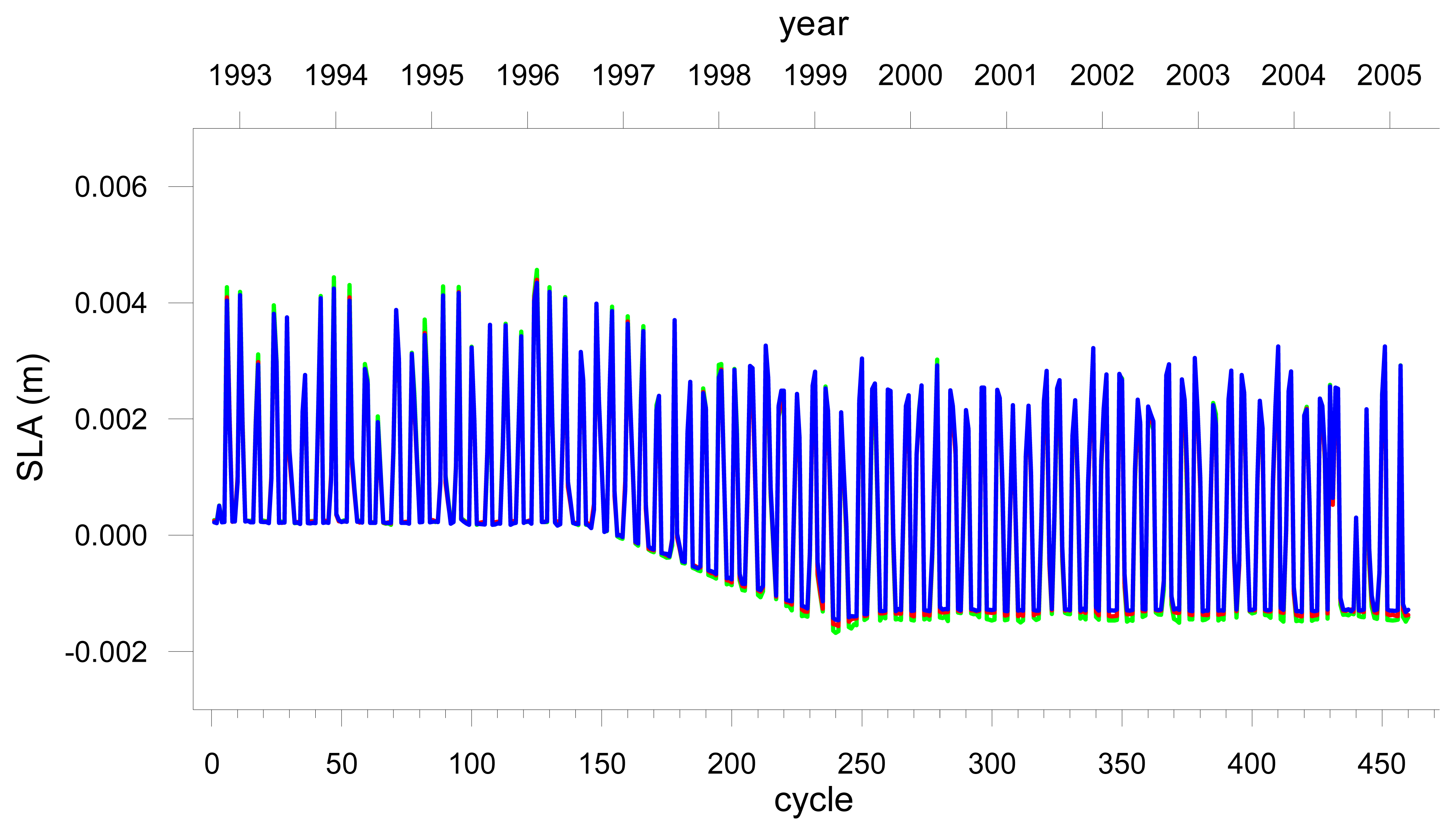
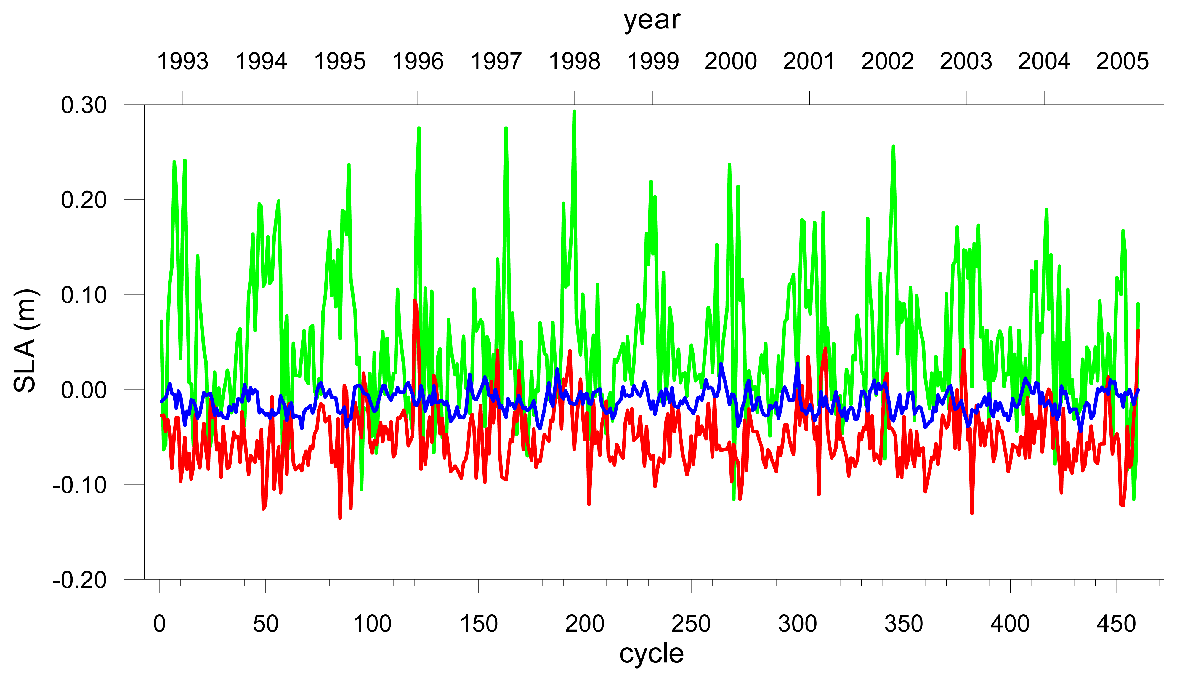
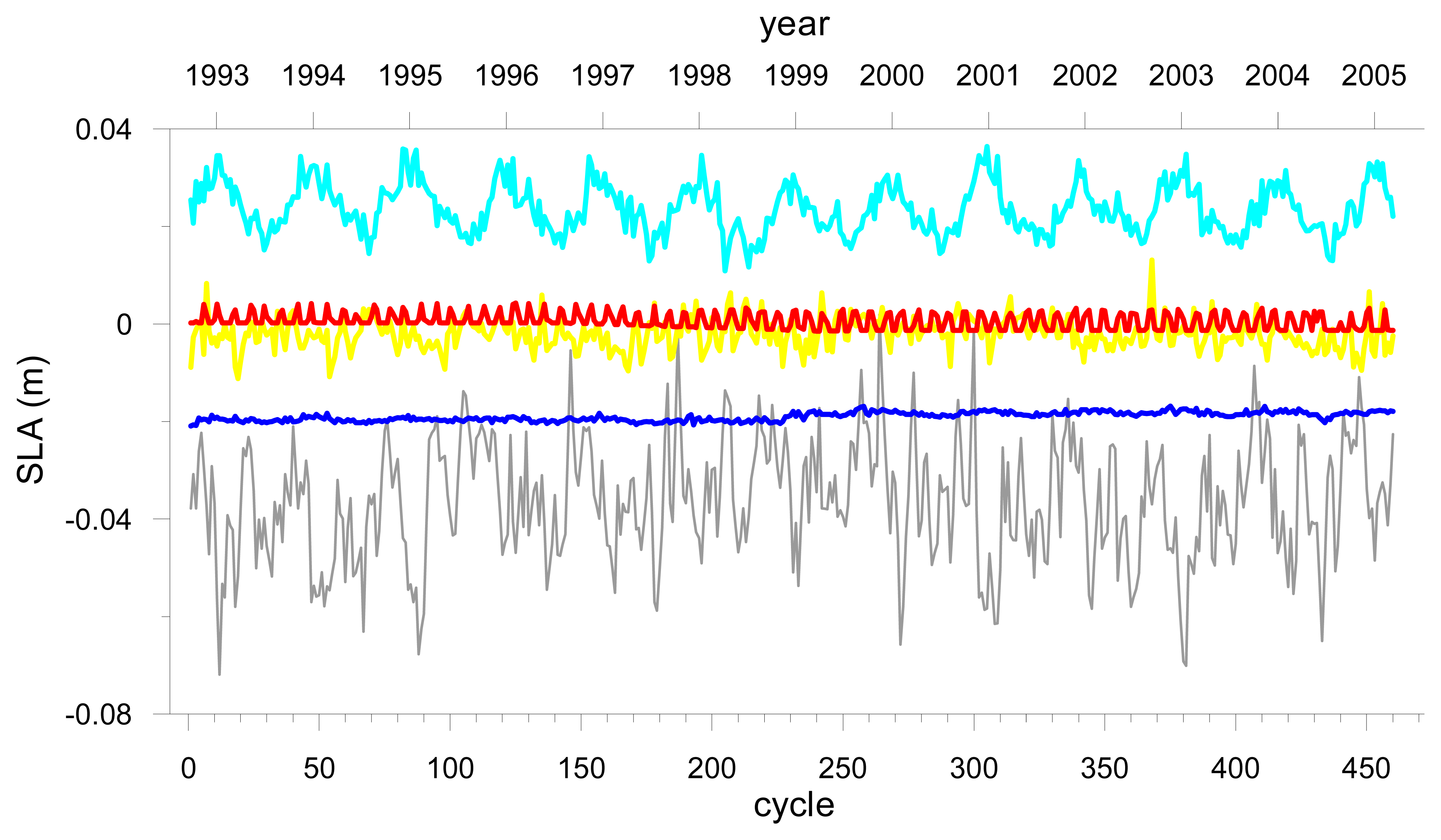
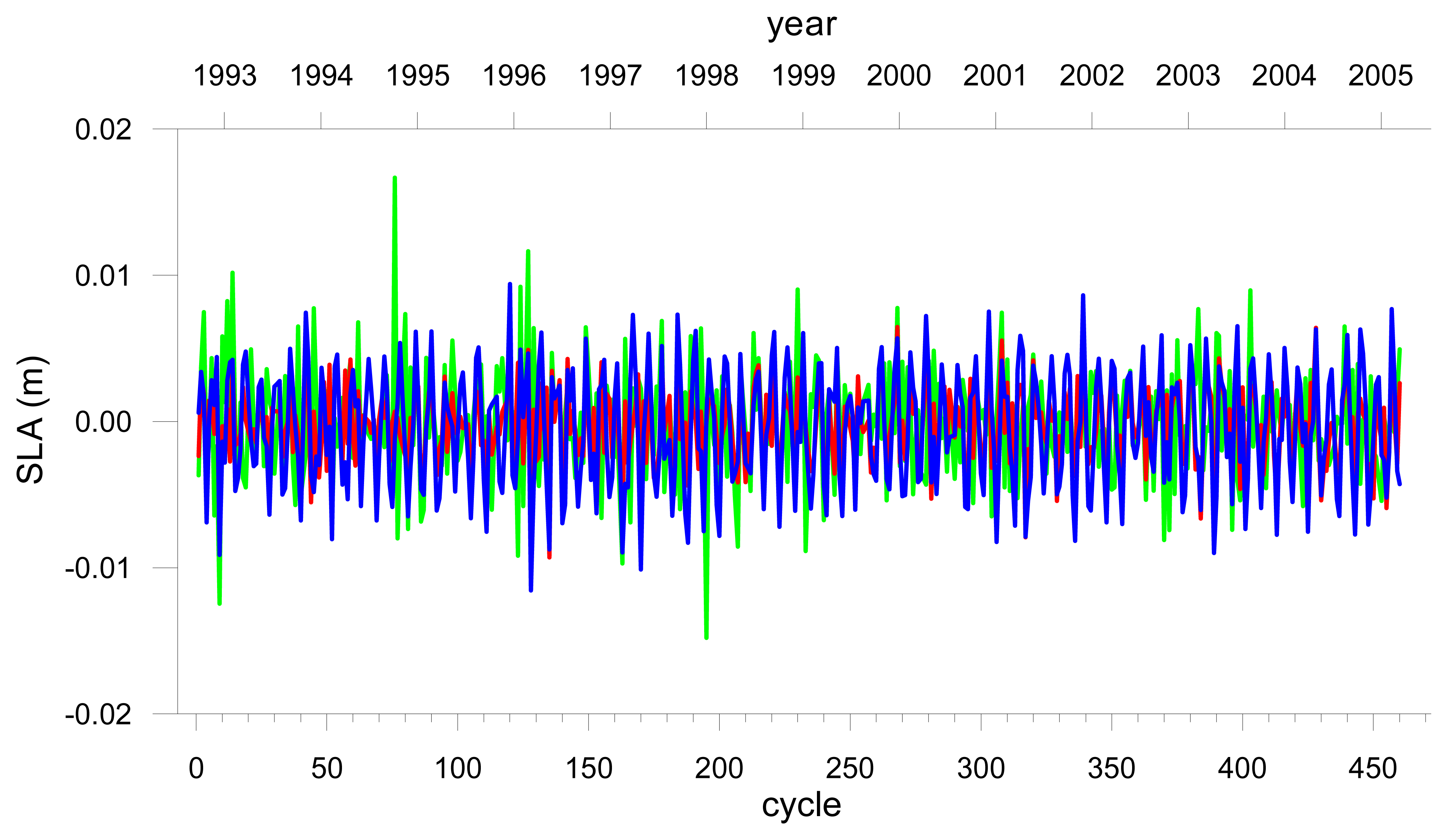
Figure 4 shows the differences between the various datasets for the Tropical region evidencing that the amplitude and shape of the signals are very different. The curve for DataSet1 - DataSet2 reveals the difference between the Chambers [27] and the Labroue [34] sea state bias models for TOPEX. DataSet1 - DataSet3 reveals the difference between the drift in the TMR as modelled by the Scharroo [26] and the Ruf [35] models. The difference DataSet1 - DataSet5 shows the effect of applying or not the inverse barometer (VRP) correction. The difference DataSet1 - DataSet7 shows the effect of using different orbits. Finally DataSet5 - DataSet4 shows the effect of applying different models (VRP-CRP) for the inverse barometer correction to the altimeter measurements. Similar plots were obtained for the Sub-Tropical and Sub-Arctic regions. The relative differences show similar signals, some of them with amplitudes increasing with latitude.

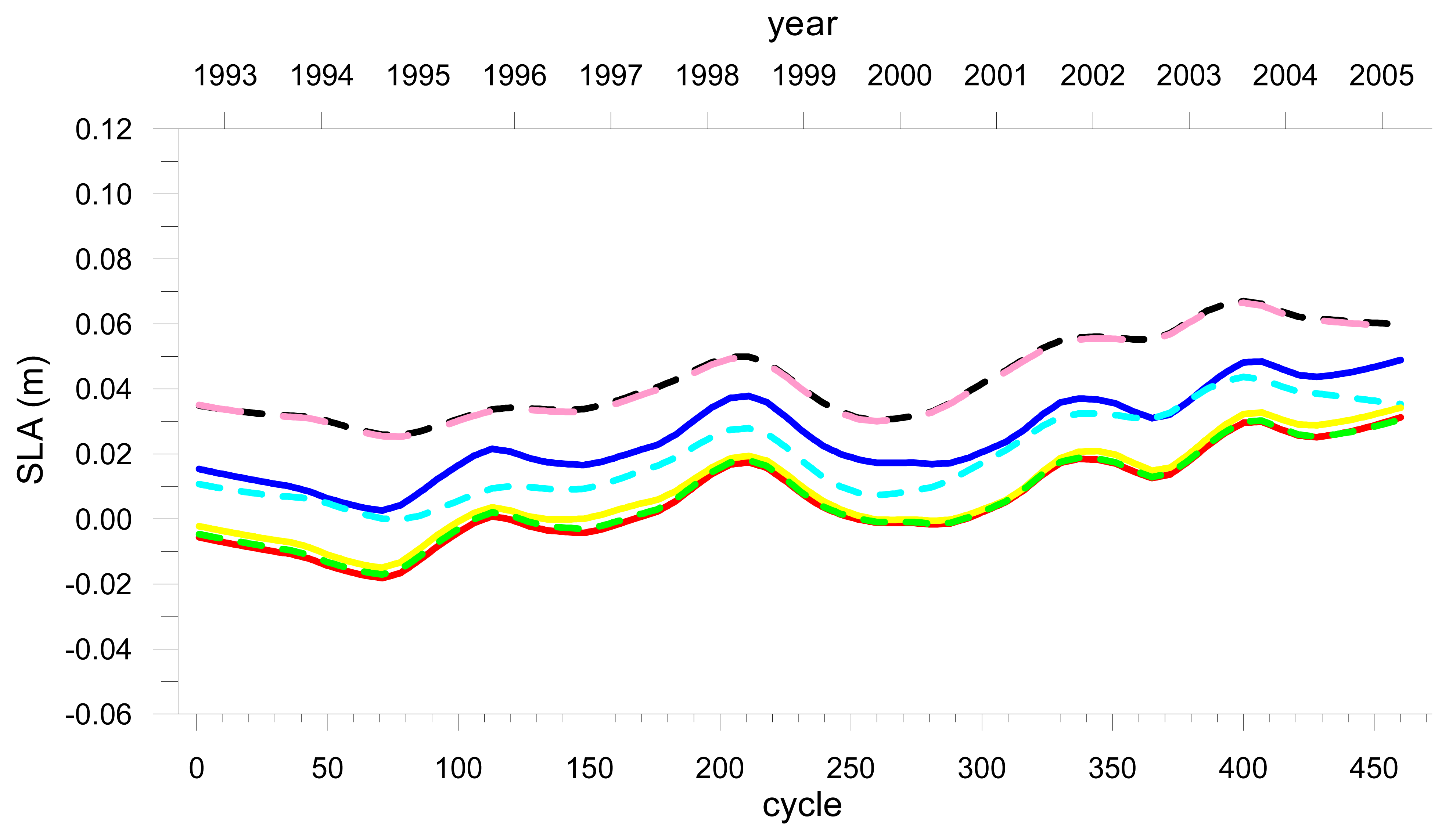
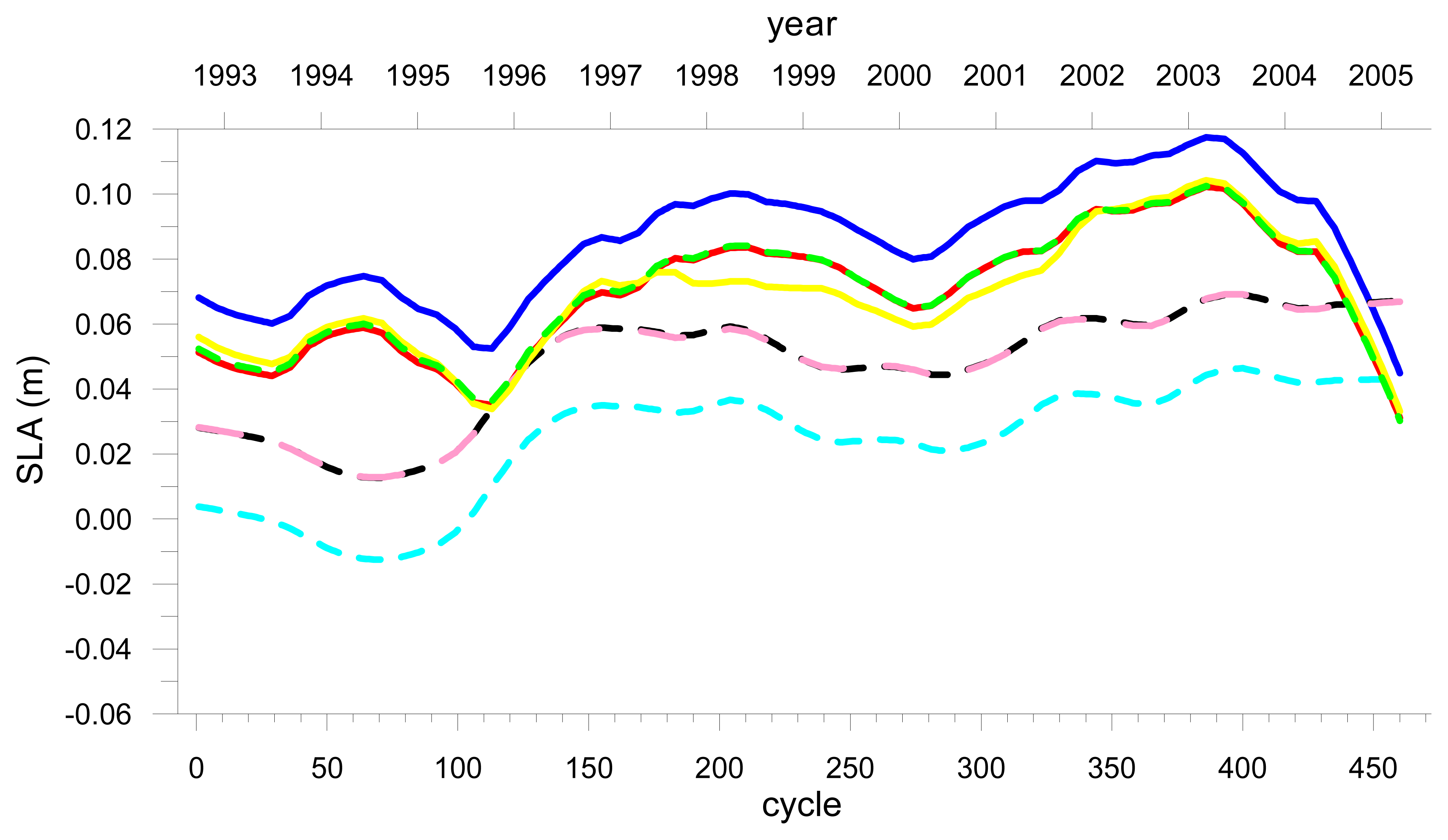
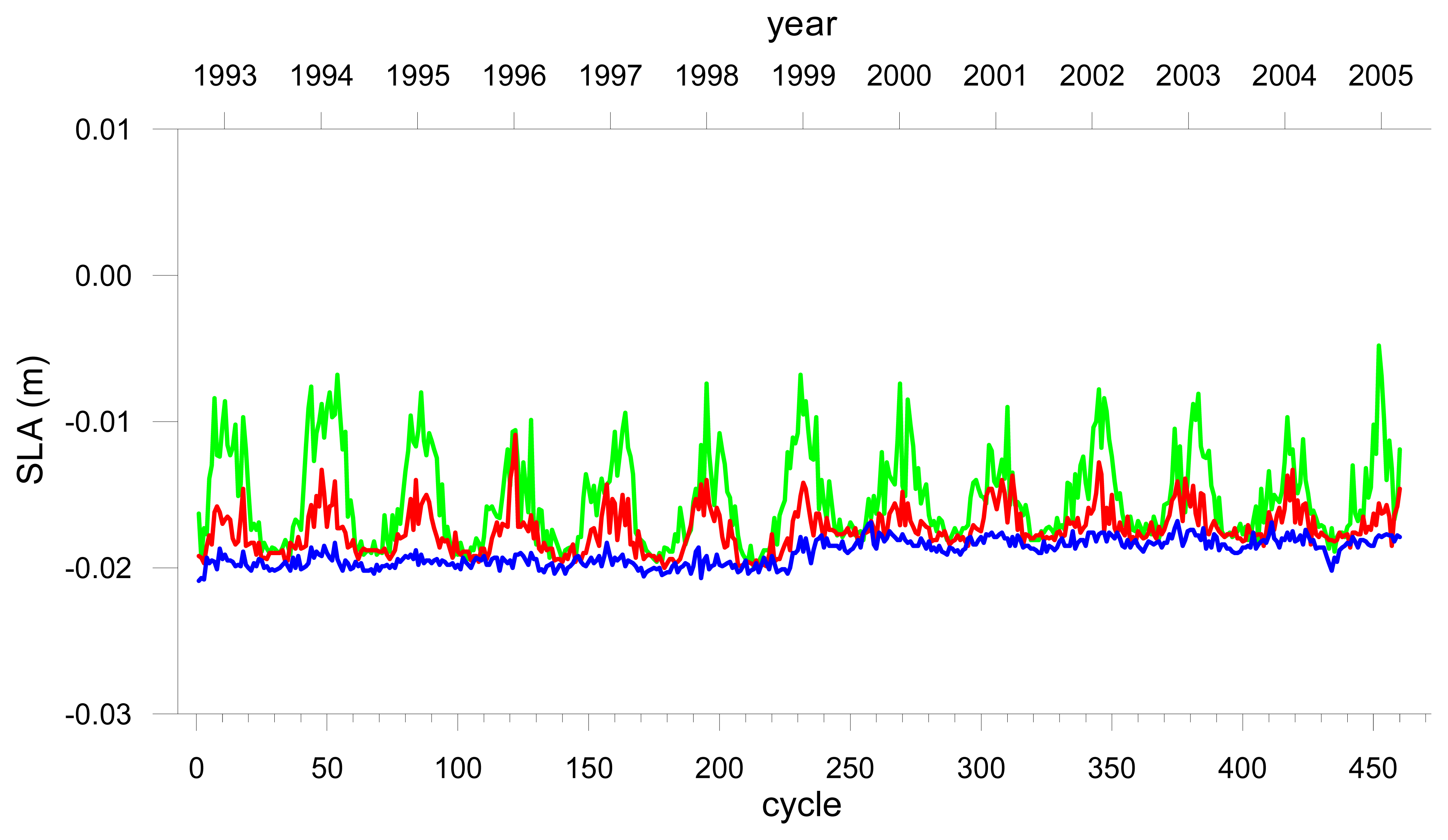
The differences between the various data sets and their dependence on the region are shown in detail in Figures 5, 6, 7, 8 and 9. Figures 10a, 10b and 10c show the SLA interannual component for each region and data set.

The sea level trends have been computed both from the interannual signal and from the original SLA time series after removing the seasonal signal (sinusoidal cycle at the annual and semi-annual frequencies). The results obtained for the linear trends (mm/yr) and respective standard errors of the regression coefficient (mm/yr), obtained by OLS fit to each time series are presented in

Table 3. Linear trends (mm/yr) and corresponding standard errors (mm/yr) obtained by OLS fit to the time series of the interannual SLA signal.

	Tropical		Sub-Tropical		Sub-Arctic
	trend	s. e.	trend	s. e.	trend	s. e.
DataSet1	3.24	0.08	1.97	0.11	3.26	0.18
DataSet2	3.07	0.08	1.86	0.11	3.22	0.18
DataSet3	3.35	0.08	2.10	0.11	3.38	0.18
DataSet4	3.14	0.08	1.82	0.09	4.14	0.13
DataSet5	2.99	0.08	1.68	0.08	3.99	0.12
DataSet6	3.00	0.08	1.69	0.08	4.01	0.13
DataSet7	3.25	0.09	1.99	0.09	3.19	0.17

and

Table 4. Linear trends (mm/yr) and corresponding standard errors (mm/yr) obtained by OLS fit to the original SLA time series (after removing the seasonal signal).

	Tropical		Sub-Tropical		Sub-Arctic
	trend	s. e.	trend	s. e.	trend	s. e.
DataSet1	3.22	0.20	2.04	0.40	3.40	0.74
DataSet2	3.05	0.20	1.93	0.40	3.37	0.72
DataSet3	3.33	0.21	2.16	0.41	3.52	0.73
DataSet4	3.14	0.17	1.83	0.18	4.14	0.23
DataSet5	3.00	0.16	1.68	0.17	4.00	0.23
DataSet6	3.00	0.16	1.69	0.17	4.02	0.22
DataSet7	3.23	0.20	2.05	0.40	3.33	0.74

respectively. It can be shown that both methods give similar results for the sea level trends; the main difference is that the first method has associated errors much smaller than the second, as it could be expected. In the subsequent analysis the values obtained with the first method were adopted.

To highlight the different results obtained for each data set,

Table 5. Linear trends differences (mm/yr) between various datasets (obtained by OLS fit to the time series of the interannual SLA signal).

	Tropical	Sub-Tropical	Sub-Arctic
DataSet1 - DataSet2	0.17	0.11	0.04
DataSet1 - DataSet3	-0.11	-0.13	-0.12
DataSet1 - DataSet4	0.10	0.15	-0.88
DataSet1 - DataSet5	0.25	0.29	-0.73
DataSet1 - DataSet6	0.24	0.28	-0.75
DataSet1 - DataSet7	-0.01	-0.02	0.07
DataSet5 - DataSet4	-0.15	-0.14	-0.15
DataSet5 - DataSet6	-0.01	-0.01	-0.02

presents the differences between computed sea level trends (computed both from the interannual signal) for selected data sets and for each of the T, ST and SA regions.

In the next four sub-sections the results for the effects of the sea state bias, radiometer wet tropospheric correction, inverse barometer correction and the orbit field will be discussed in detail. Before discussing the results it should be emphasised that all 21 time series have been processed using exactly the same methodology in order to highlight the effects of using different geophysical corrections and orbit fields.

4.1. Sea state bias

The development of SSB models for the various altimeter missions has been a subject of major research. The sea state bias correction is composed of several parts: the electromagnetic (EM), the skewness and the tracker biases. The EM is theoretically only a function of the frequency of the radar altimeter EM pulse. The skewness and the tracker bias are due to inaccurate tracking of the waveform by the on-board tracker and also depend on the sea state and on the altimeter frequency [1]. Since all components depend on the sea state and on the altimeter frequency, in practice the combined SSB effect for each altimeter is estimated as a function of the sea state parameters significant wave height (SWH) and wind speed (WS).

Most of the methods which have been used for determining the SSB correction fall in two main categories: parametric and non-parametric methods. The SSB is estimated by fitting an empirical model on altimeter-derived SSH differences, either at crossover points or along collinear tracks.

Parametric methods often assume an empirical relation between SSB, SWH and WS of the form (6),

$$\mathit{\text{SSH}}=\mathit{\text{SWH}}(a_0+a_1\mathit{\text{SWH}}+a_{2}WS+a_{3}W{S}^2)$$

(6)

where SSB is the sea state bias in metres, SWH is the significant wave height in m and WS is the wind speed in m/s. The model parameters for each altimeter are estimated by a least squares fit of the model to sensor data for a given period. Gaspar [42,43] and Chambers [27] are examples of parametric SSB models developed for TOPEX using 4 parameters according to (6).

Non-parametric techniques have been developed for estimating the SSB from altimeter data themselves and applied to most satellite missions including TOPEX [44-46]. Each model is a look-up table expressing the two-dimensional SSB dependence on the SWH and WS fields. The non-parametric SSB model used in this study for the generation of DataSet2 is the most recent TOPEX solution obtained by Labroue et al. (Labroue, personal communication).

Scharroo et al. have been developing the so-called hybrib methods [47,48], consisting of an extension of the direct estimation method of the SSB from residual SSHs [49] through a parametric fitting followed by a successive smoothing of the residuals. The hybrid method essentially produces a non-parametric SSB model in the form of a smooth grid in the two-dimensional space determined by two sea state parameters.

The Chambers SSB [27] was developed as a correction model to the Gaspar BM4 model, [43] provided in the GDR-Ms which has been derived from TOPEX A data only and was found to be inadequate when applied to the entire TOPEX mission. Our results for the North Atlantic (not shown here) reveal that the difference between these two models has a strong annual latitude dependent signal, being almost an order of magnitude higher for TOPEX B than for TOPEX A. The effect on regional sea level trend of the difference between these models (with no TOPEX A/B bias applied) is 0.6 mm/yr in the Tropical region, 0.9 mm/yr in the Sub-Tropical region and 1.3 mm/yr in the Sub-Arctic region, which is in agreement with the Chambers [27] results, who reported a global increase on sea level rise of 1.1 mm/yr due to the difference between the two models.

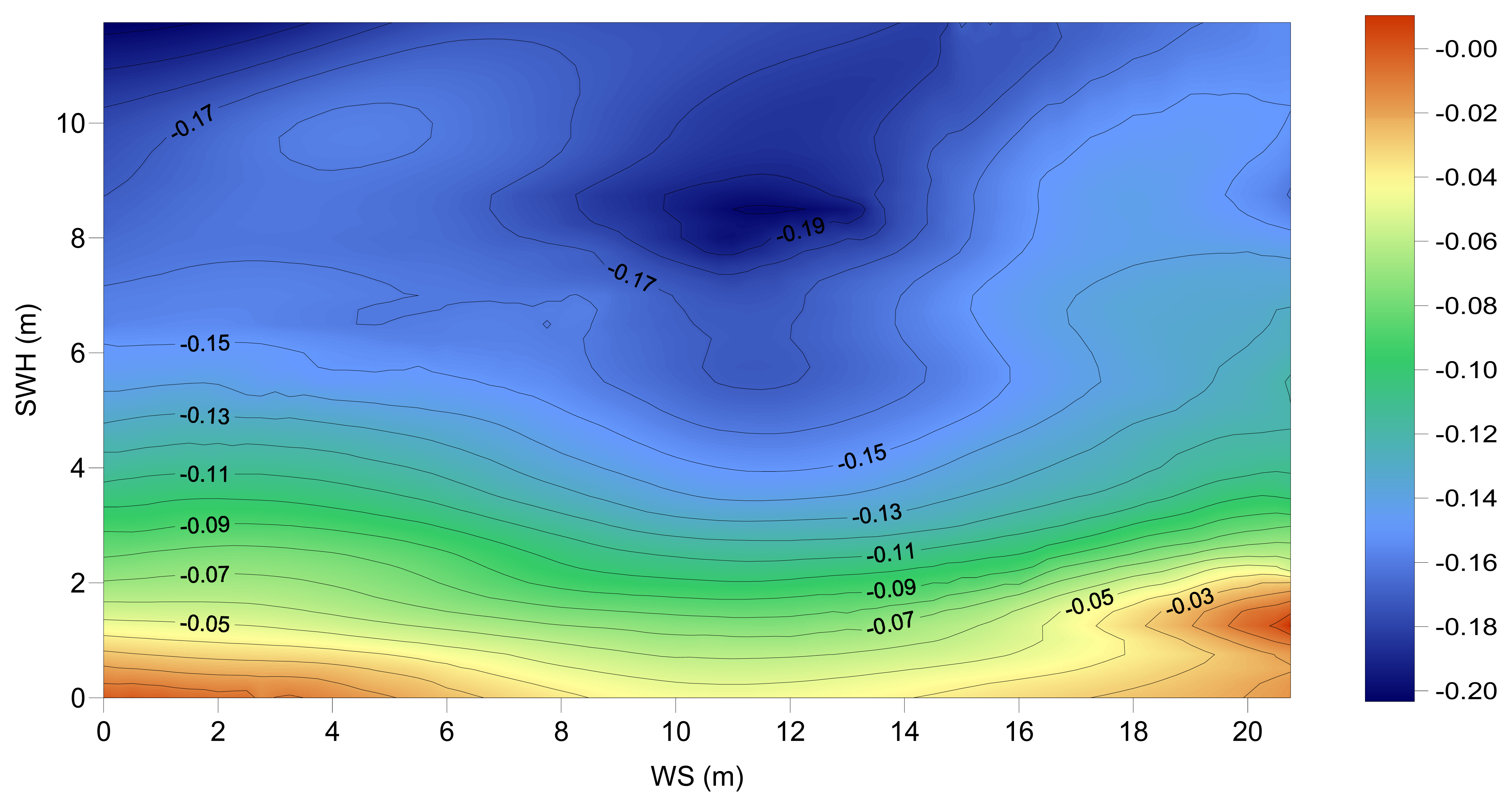
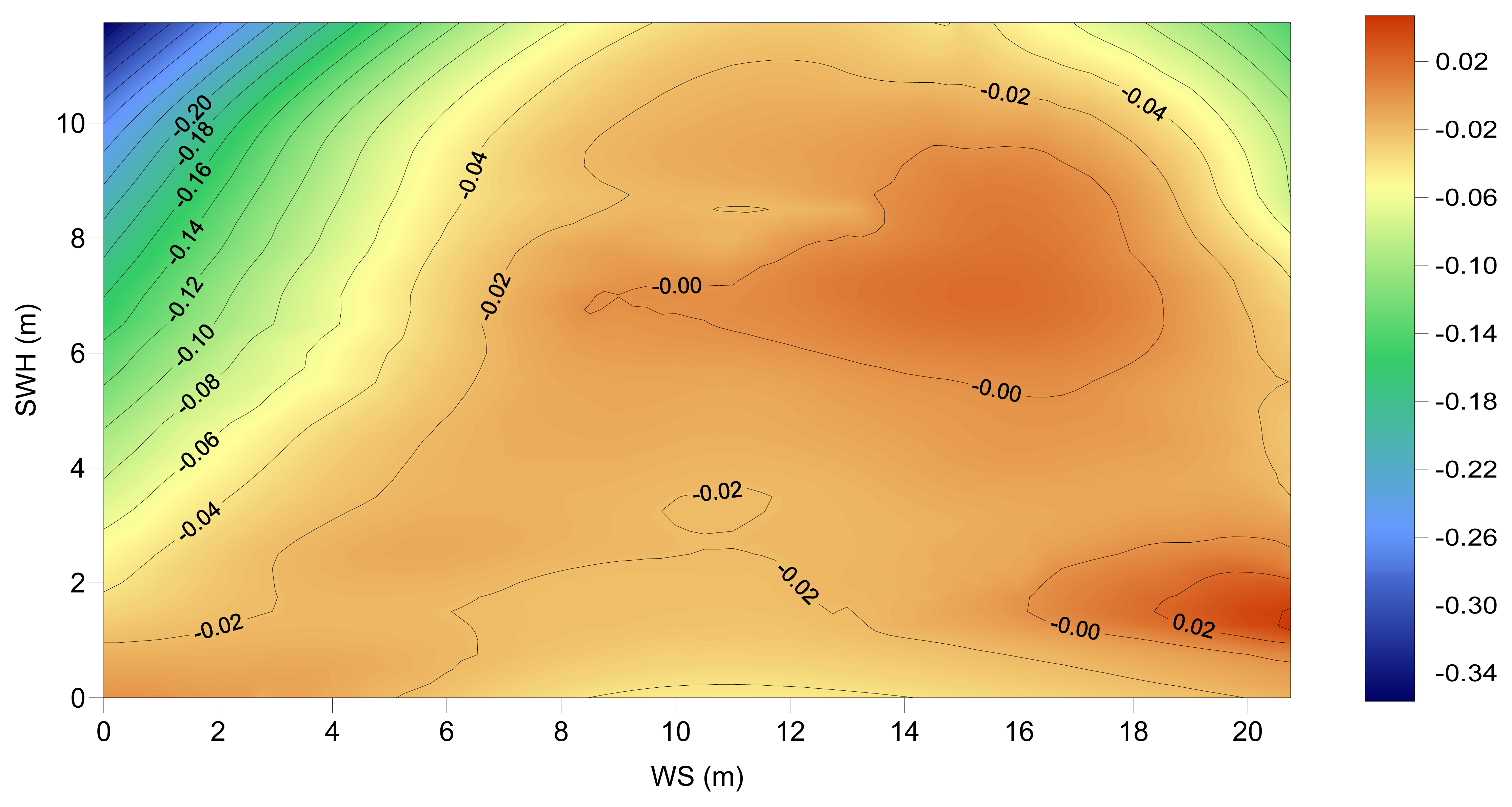
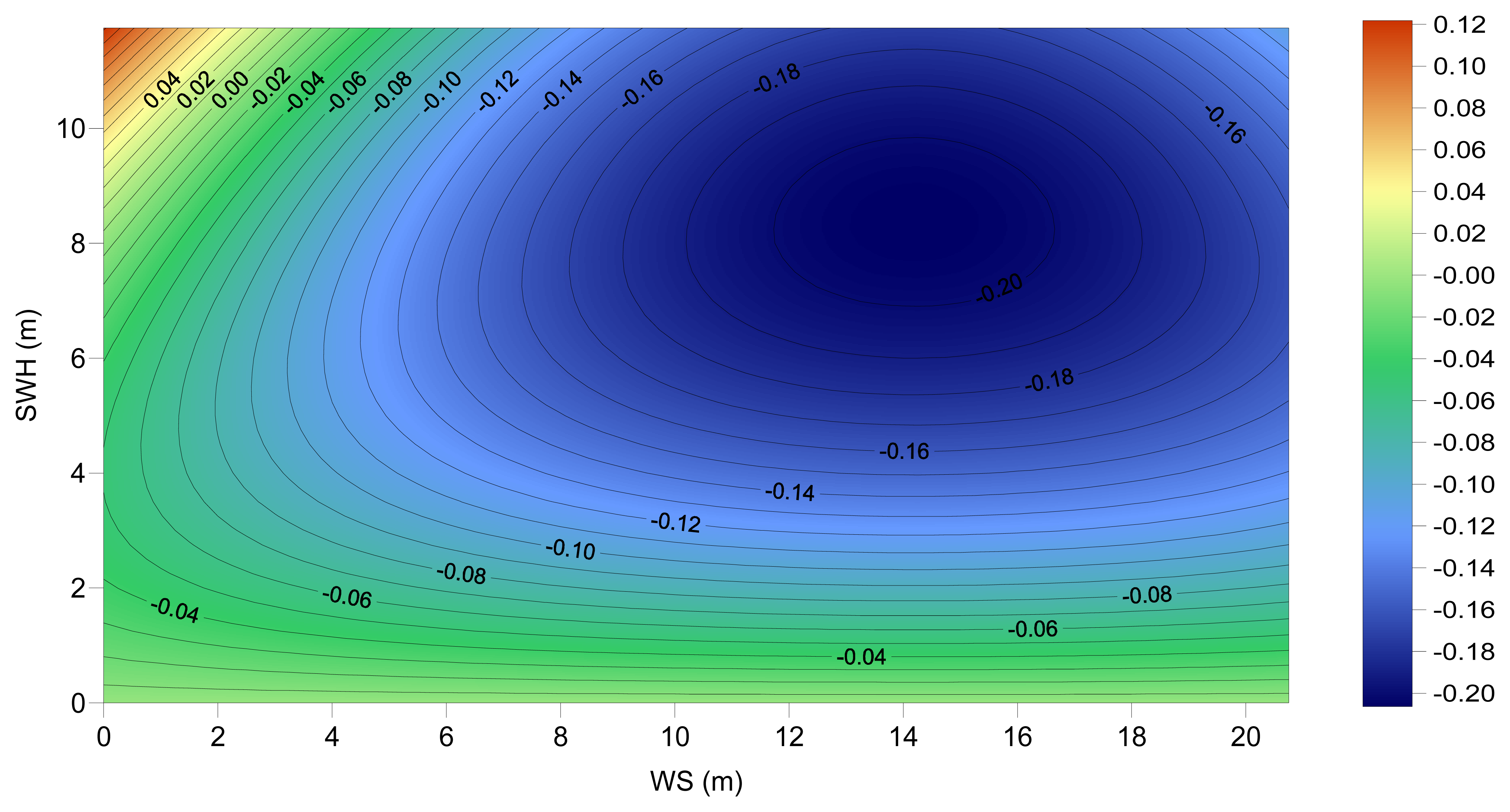
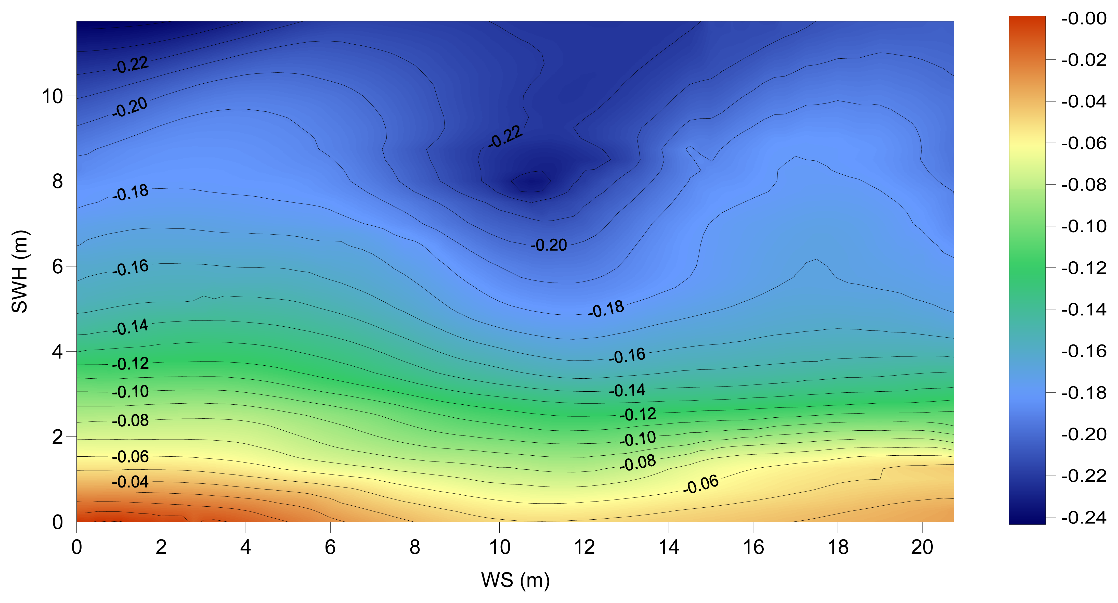
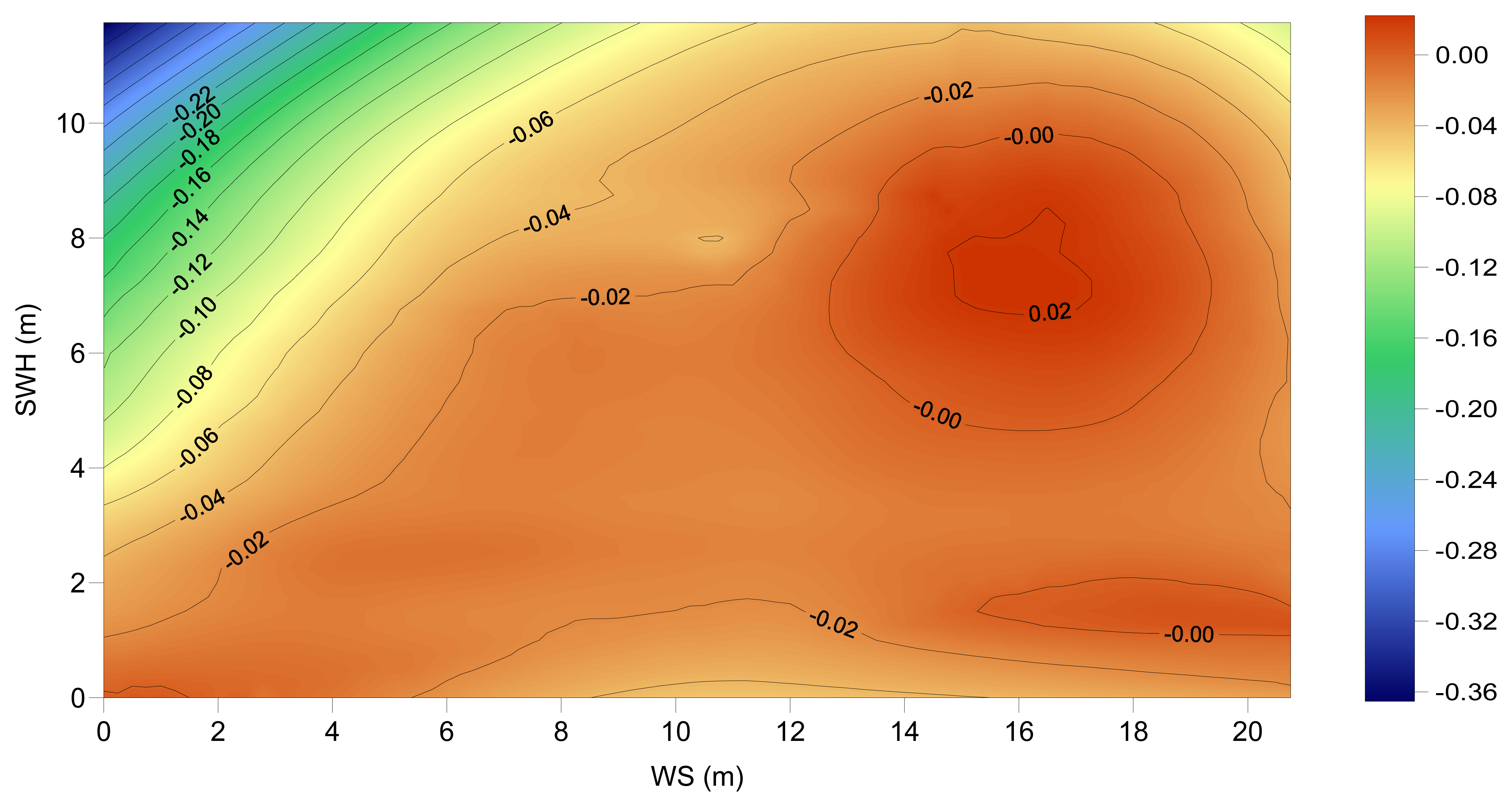
Both the Chambers and the Labroue models used in this study have been developed as separate models for TOPEX A and TOPEX B, derived from data from each of the instruments, aiming to take into account the different response of the TOPEX A and B altimeters to the sea state. The two TOPEX A models and their differences are shown in Figures 11a to 11c; the corresponding models for TOPEX B are shown in Figures 12a to 12c. These figures evidence that there are major differences between the models. These differences are explained by the different computation procedures associated with each model: the non-parametric method allows a better fit to data than the parametric one. Very extreme values of the differences occur at sea state conditions that are less frequent, therefore with a worse data sampling in the adjustment procedure. The similarity between these models is higher for low values of SWH (up to ∼4 m), almost irrespective of the WS value.

Our first comparisons of time series of sea level anomalies derived with different SSB models, without applying any a priori TOPEX A/B bias, showed small but clear biases of few millimetres between the two altimeters. It has been pointed out by various authors [27,2] that the TOPEX A/B relative bias depends on the model adopted for the SSB correction. While different values have been reported for this bias when using the Chambers model, [28,2], no result has been published yet for the most recent Labroue model.

Motivated by these results we developed a simple method to determine the TOPEX A/B relative bias for the SSB models used in this study. Using the same corrections applied to DataSet1 and DataSet2 (apart from the TOPEX A/B bias) global mean sea level values were computed using an equal-area weighted average [2]. Differencing the means over the 10 cycles before and after the A/B switch produced a TOPEX A/B bias of 2 mm for both the Chambers and Labroue models. This value agrees, within 1mm range, with the values referred by [28] and [2], the last determined by calibration with tide gauges. The same method proved to be efficient in the determination of the TOPEX A/B relative bias for other SSB models (not shown here).

The derived biases were added to the TOPEX B SSB values in the generation of both DataSet1 and DataSet2. Equivalently, they could have been subtracted from the corresponding TOPEX B sea level anomalies. Note that, since all remaining datasets used in this study (DataSet3 to DataSet7) use the same SSB (Chambers) model, the same TOPEX A/B bias of 2 mm has been applied to all of them.

Our results show that, after applying the above mentioned biases, the pattern of the amplitude of the cycle mean differences between the Chambers and the Labroue models (Figure 5) is now very similar for TOPEX A and TOPEX B and the A/B transition is almost flat. The signal of the differences also shows a strong annual latitude dependence.

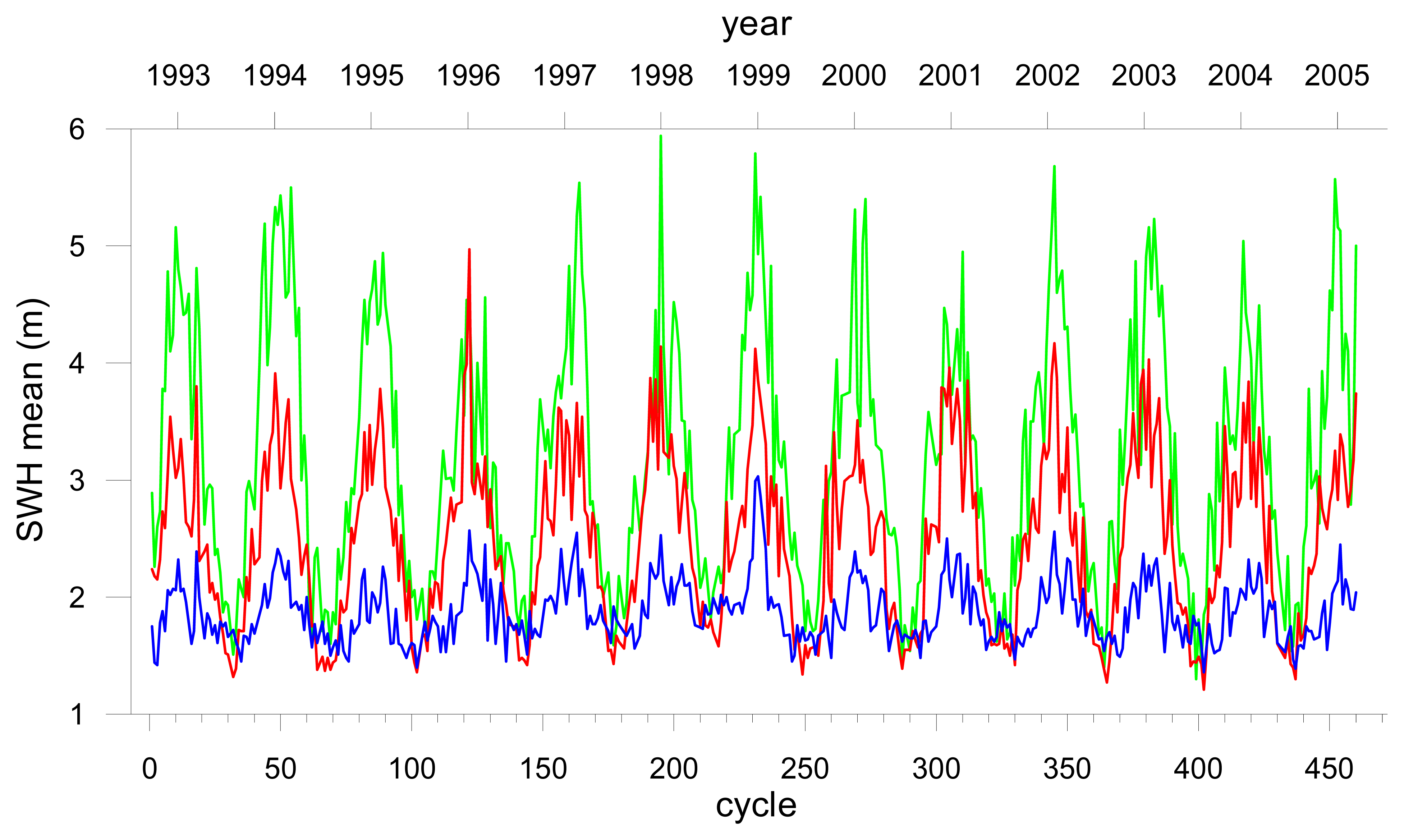
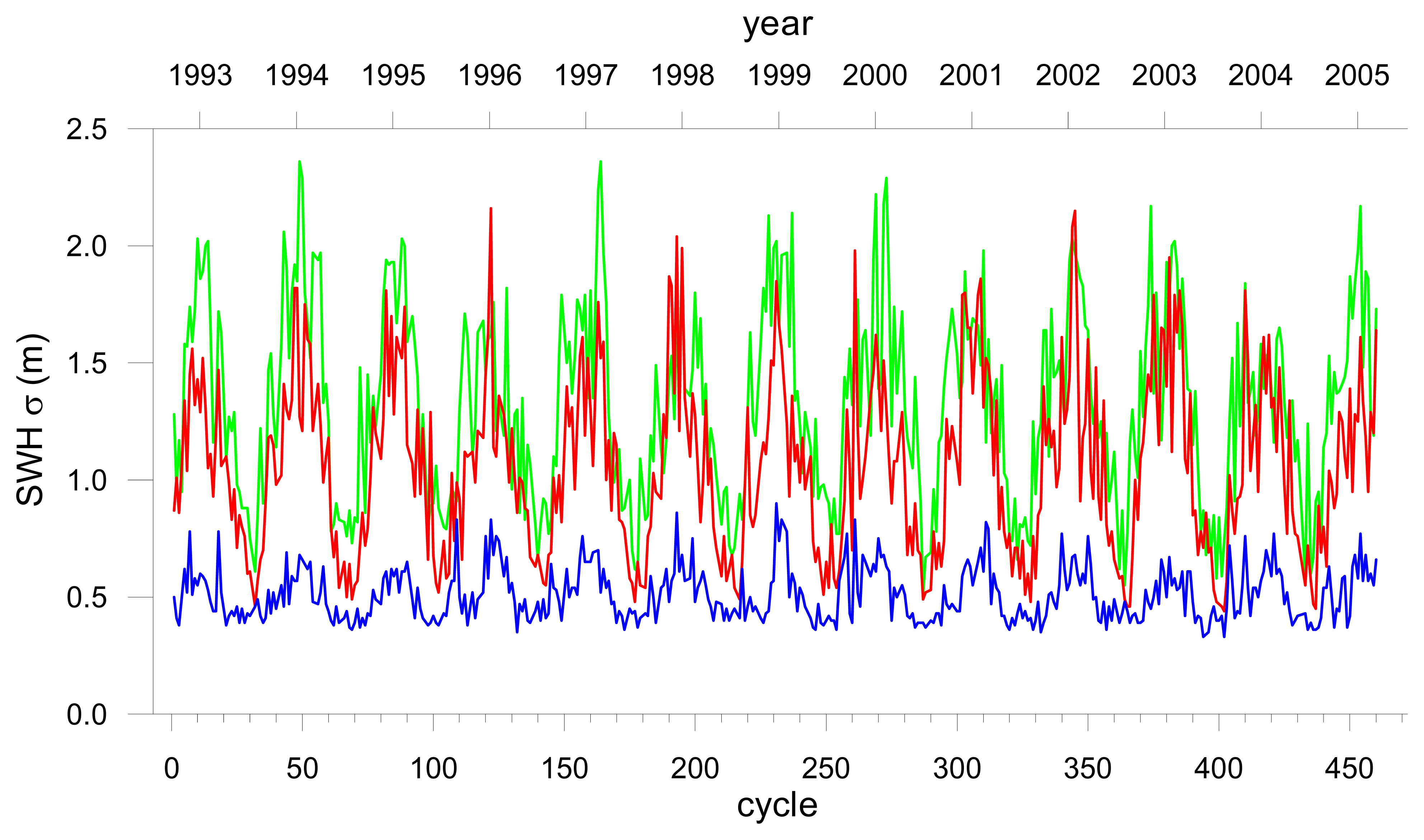
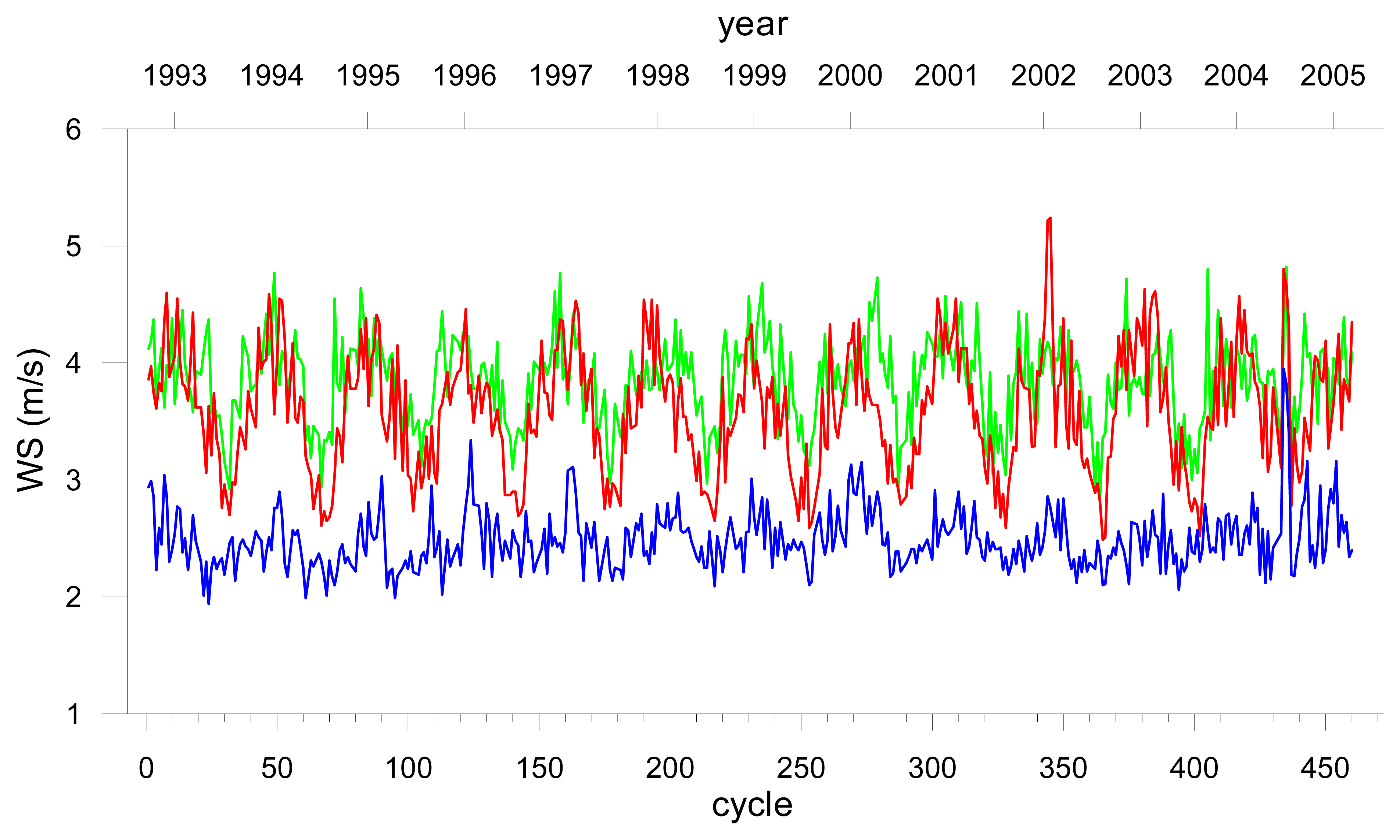
The seasonal and latitudinal dependence is explained by the fact that both SSB corrections are empirical models, functions of the significant wave height (SWH) and wind speed (WS), both measured by the altimeter. Both fields have a strong annual variation with intensity and variance increasing with latitude, particularly during the boreal winter months. This is clearly shown in Figures 13 and 14, representing the time evolution of the mean and standard deviation of the SWH and WS fields respectively, for each cycle, during the analysed period and for the three studied regions. 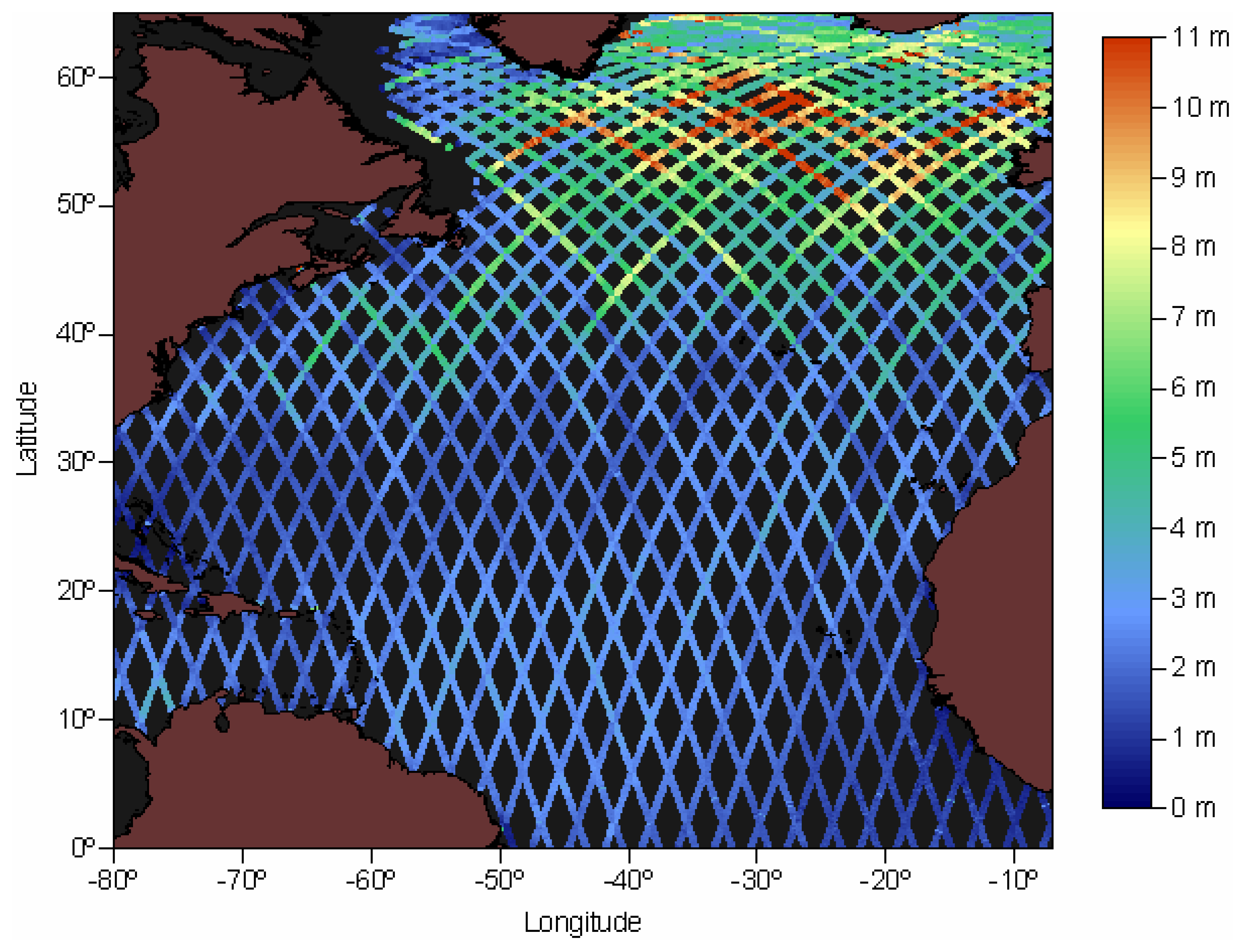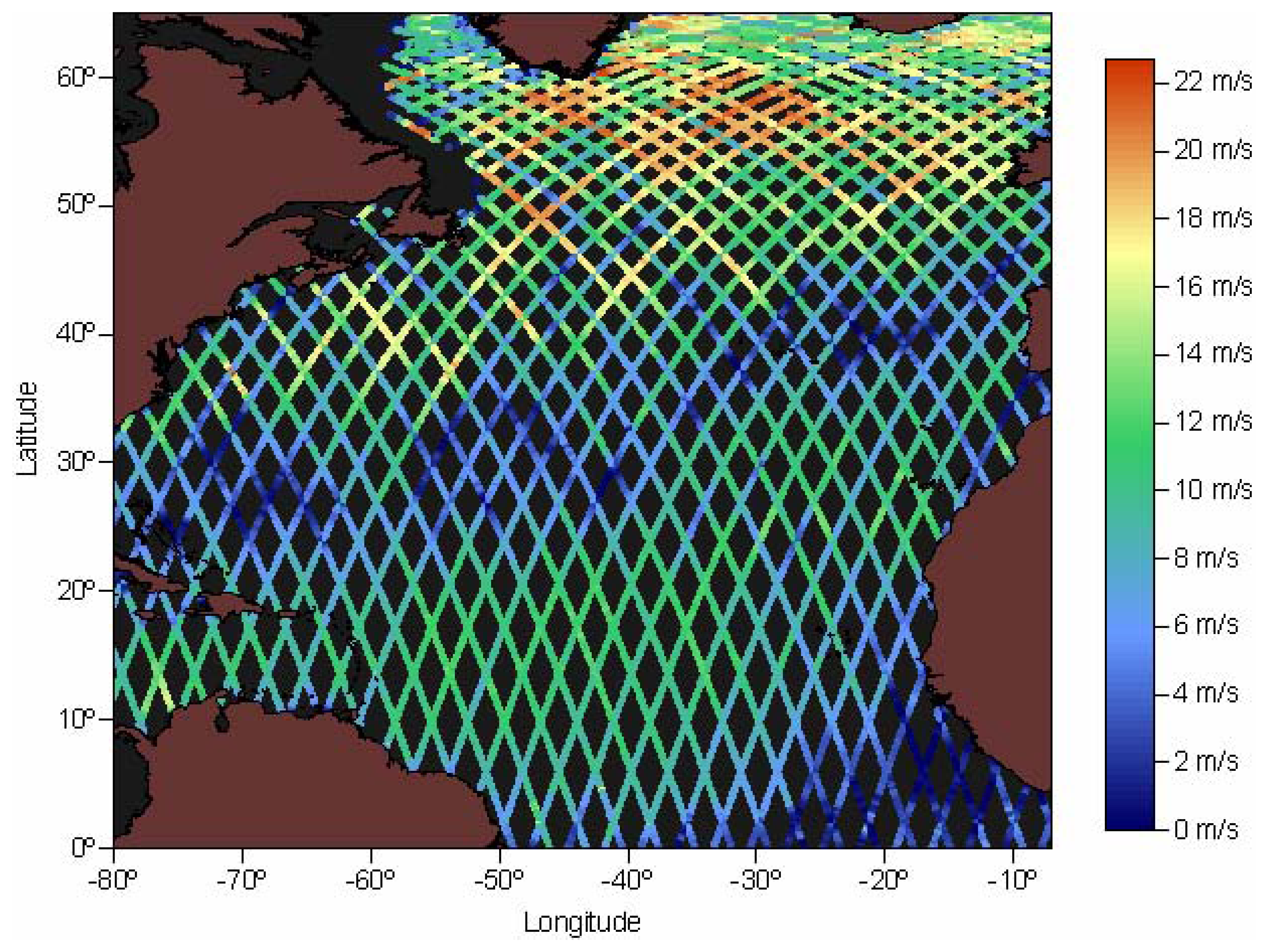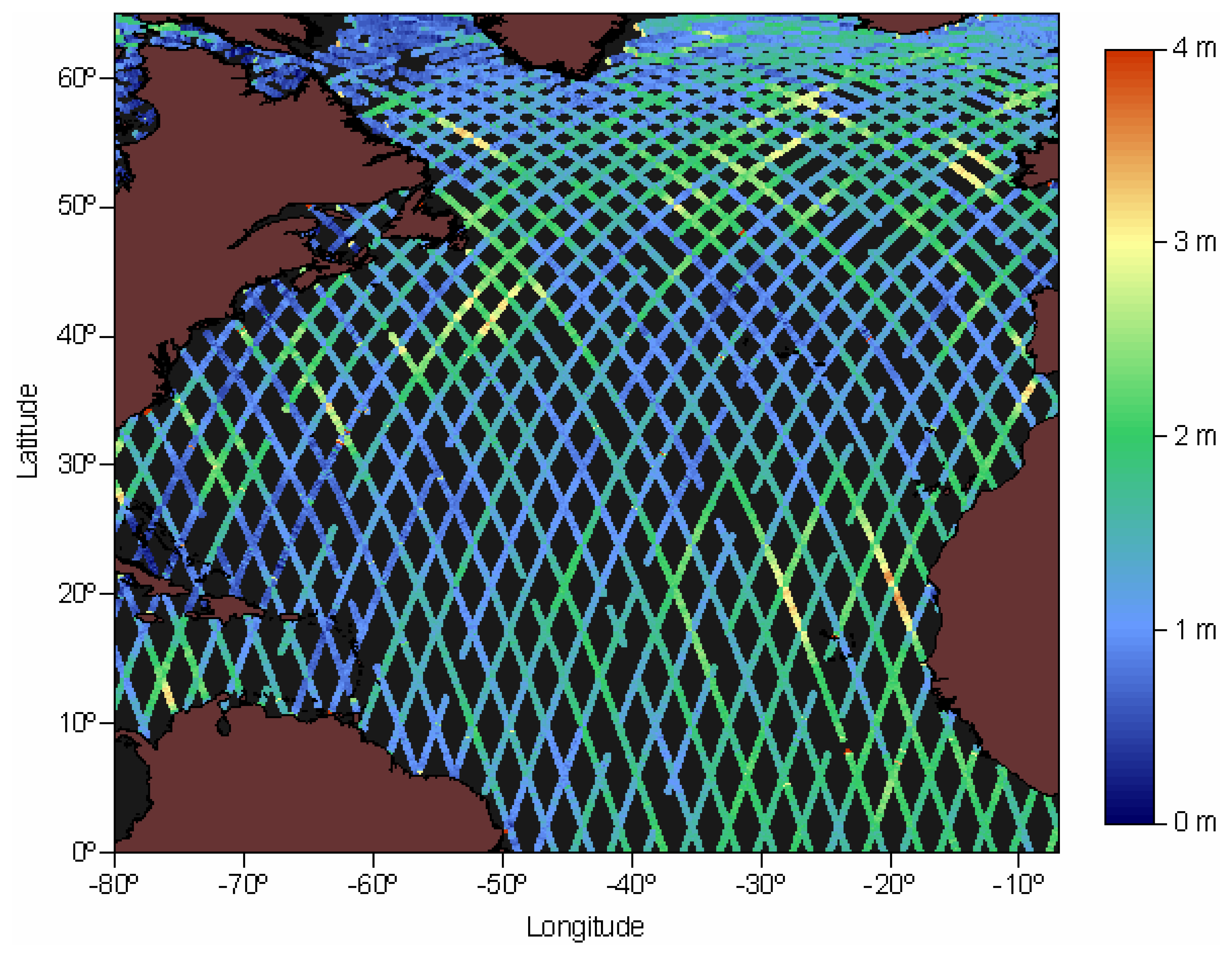Figures 15 and 16 illustrate the spatial patterns of the same fields for representative North Atlantic winter and summer conditions respectively. Figure 15 shows that during a typical winter cycle the amplitude of both SWH and WS fields have a strong latitudinal dependence with maximum values in the Sub-Artic region. On the contrary, Figure 16 shows that during a characteristic summer cycle the intensity of the same fields, although exhibiting some geographical patterns, does not possess a clear latitudinal dependence.

Figures 11c and 12c show that, for a large range of SWH and WS values the mean difference between the models is close to -0.02 m, in agreement with Figure 5. Typical values for winter conditions in the Sub-Arctic region are around 5-6 m for the SWH (Figure 13a) and 13-15 m/s for the WS (Figure 14a). For these mean extreme values in the study region the difference between the models lies in the region where the differences are closer to zero, in agreement with the pattern of the mean cycle differences shown in Figure 5.

The regional dependence of the SSB does not only influence sea level variations. Dong and coworkers [50] refer to the SSB influence in the estimation of the bias between different satellites. It is also known that the ionospheric correction derived from dual-frequency measurements at the Ku and C frequencies is influenced by any errors in the adopted Ku-band and C-band SSB models. However, while a SSB model derived from an “imperfect” ionospheric correction may not represent the “true” SSB, it will attempt to minimise the errors in the SSH (and in the ionospheric correction) related to the sea state [27].

According to Table 5 the difference between the two adopted SSB models induces a small change in sea level trend of 0.0 to 0.2 mm/yr in the considered regions. Apart from this linear trend, the interannual signal derived for both data sets reveals similar patterns within each region (see Figures 10a, 10b and 10c, green and blue curves). Note that the relative bias between TOPEX A and B when using the two SSB models (Figure 5) is of the order 1 mm, within the computation error, indicating that the two data sets seem to be consistent with respect to the TOPEX A/B transition. Further insight into the analysed models with respect to the continuity of TOPEX A and TOPEX B solutions can only be obtained through model comparisons at absolute calibration sites or with tide gauge data.

4.2. Radiometer wet tropospheric correction

The GDR-Ms provide the radiometer wet tropospheric correction (wet_cor) as computed from the measured TBs of the 3 TMR channels (18 GHz, 21 GHz and 37 GHz). Several authors have reported drifts in the TBs of some of these channels and published correction models to account for these effects in the wet tropospheric path delay, [51,35,52,26]. The first two authors report a global effect on sea level change of about 1.0-1.5 mm/yr due to this instrument drift, between October 1992 and December 1996.

Ruf [35] and Callahan [52] have derived drift models for the 18 GHz TBs using a linear function of the TBs up to a certain date (late 1996 and early 1999 respectively) followed by a constant correction. The drift model used in this study for the generation of DataSet3 is a modified version of the Ruf model, as explained previously.

Apart from refining the 18 GHz model by using a piecewise linear function of the TBs, Scharroo et al. also derived drift models for the other two channels (21 GHz and 37 GHz). In addition, their model also takes into account the yaw state corrections to the TBs of all the three TMR channels.

Our results show that the effect on the North Atlantic sea level variation of using the two TMR drift models (Scharroo and Ruf) is of 0.1 mm/yr (Figure 6 and Table 5). Although non negligible this effect is much smaller than the effect of unmodelling the drift itself, which, considering Scharroo's model is of 0.4 mm/yr. Apart from the effect of using different drift functions, Figure 6 shows the effect of the T/P yaw state corrections, which range from 0 to 5 mm. These corrections were not applied to DataSet3 since they were reported after the development of the Ruf's model. In spite of the variability introduced in the derived SLAs, the yaw state corrections do not affect long-term sea level trend.

The effect of the TMR drift on sea level studies is highly dependent on the length of the analysed altimeter time series. Most TMR drift models, including the two analysed here, consider that the TMR drift after 1999-2000 is approximately constant. Therefore, the longer the time series the smaller the effect will be. In Figure 10 the effect on sea level interannual variation for the three different North Atlantic regions is shown by comparing the green (DataSet1) and red (DataSet3) curves. Although some latitudinal dependence could be expected related with the spatial variability of the various TBs, these figures and the results presented in Tables 3 and 5, show that the latitudinal dependency is not significant.

In spite of instrumental problems in the onboard microwave radiometers, affecting the wet tropospheric delay derived from the TBs measured by these instruments, provided these are properly modelled and accounted for, the radiometer derived wet_cor is still more accurate than the corresponding ECMWF model correction. For TOPEX, the TMR model provides a path delay correction with the accuracy better than 1.1 cm, even under the worst conditions of variable clouds and wind, [53]. Although the ECMWF model correction has been improving, several modifications introduced discontinuities in the model, making it unsuitable for use in sea level studies, [25,26].

4.3 Inverse barometer correction

Results show that the inverse barometer is the correction with the largest impact in the shape of the SLA time series for a given region (Figures 4, 7, 8 and 10). There is no consensus between the research community whether or not the IB correction should be applied to the altimeter data for sea level studies, [9,36,6], although this discussion was mainly related to the observation that an inverse barometer correction using a constant reference pressure creates unrealistic signals, since the mean correction is no longer zero, which is not consistent with ocean mass conservation [36].

In this study three different IB models have been compared, one that makes use of a constant reference atmospheric pressure (CRP) of 1013.3 mbar (DataSet4), one that uses a variable reference surface atmospheric pressure (VRP), interpolated from global average values obtained from the CNES/CLS (DataSet5) and the so-called combined-MOG2D model (DataSet6). In the computation of the VRP model, the values of P̅ have been smoothed using a (2-day)^-1 cut-off frequency. However it was found that the smoothing does not affect the mean sea level determination since the maximum difference in the values of P̅ is 0.7 mbar, which causes a maximum SLA change of 7 mm.

Figure 8a shows that the amplitude of the differences between the VRP and the CRP models can be as large as 2.5 cm and exhibits a strong seasonal signal. As expected, these differences are not region dependent, since the actual difference between the two models resides in the use of the constant value of 1013.3 in Equation (3) instead of the value of P̅ given by Equation (5) and the value of P̅ is global by definition, [36]. Both models have a similar impact on sea level trend with the VRP model giving slightly smaller trends by about 0.13 mm/yr (Tables 3, 4 and 5). Using only four years of T/P data [36] had found that globally the second model would give sea level variations 0.4 mm/yr smaller than the first one.

The pattern of the differences between the combined-MOG2D and the VRP models presented in Figure 8b is quite different from the previous two models. Now the seasonal signal has disappeared, as it could be expected since both models use the same modelling for the long wavelength atmospheric effects given by the inverse barometer response. This figure is now dominated by the high frequency effects modelled by the MOG2D barotropic model. Carrère et al. [37] found that the use of this model reduces the T/P crossovers variance by more than 15% with respect to the classical inverse barometer correction. The corresponding curves for the interannual signals shown in Figure 10 (dashed pink and dashed black curves) are almost coincident.

Figures 7a and 7b reveal the impact of the application of the IB correction from two of the mentioned models (CRP and VRP) on the shape of the corresponding SLA time series, showing the expected latitudinal dependence, related with the spatial variability of the pressure fields. Similar results were obtained for the combined-MOG2D model.

Figure 10 reveals that the shape of the interannual signal of an SLA time series without any IB correction (DataSet1) and the corresponding signals of the IB corrected ones (DataSet4, DataSet5 and DataSet6) are significantly different, particularly for high latitudes.

In global studies IB corrected SLA time series tend to give smaller sea level trends than the corresponding non IB-corrected, [25,36]. However, this work shows that in regional studies this is not always true. For the Tropical and Sub-Tropical regions the difference in sea level trend determined by a non IB-corrected series (DataSet1) and any of the IB-corrected ones (DataSet4, DataSet5, DataSet6) is in the range of 0.1 mm/yr to 0.3 mm/yr (Table 5). However, for the Sub-Arctic region it is significantly different, of the order of -0.8 mm/yr.

Atmospheric pressure variability exhibits a strong latitudinal dependence with the lowest values at tropical latitudes (∼2 mbar) and the highest values (∼15 mb) at polar latitudes, [54]. Thus the differences in the sea level interannual components related to whether the IB correction is applied or not to the altimetry measurements are most noticeable for the northern region.

The interannual components for the Subarctic region show a significantly different behaviour for IB-corrected and not corrected datasets. The sea level series for which the IB correction has not been applied departs significantly from the IB-corrected series for three distinct periods: near 1995, near 2000 and after mid-2003. These periods are associated with significant anomalies in the atmospheric patterns over the North Atlantic which influence the inverse barometer response of sea level.

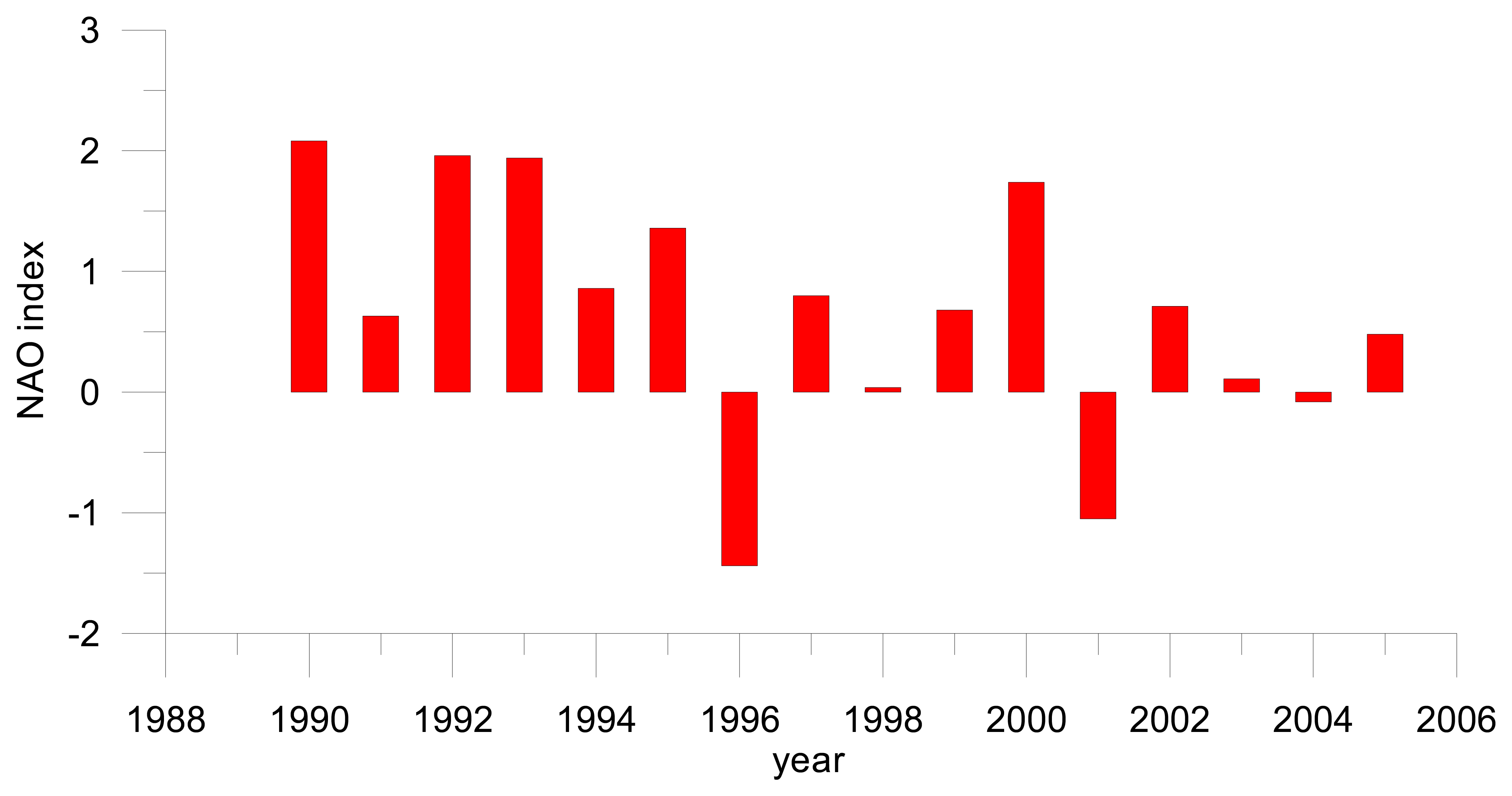
The North Atlantic Oscillation (NAO) affects the sea surface height through a direct hydrostatic response to changes in the pressure field and indirectly through wind, ocean circulation and heat flux forcings [55-58]. The NAO index (Figure 17) switched from one of its highest positive values in 1995 to one of its most negative value for this century in 1996; a similar switch, but not as prominent, occurred in 2000-2001. We believe that the different shape of the IB-corrected and non IB-corrected curves shown in Figure 10 (particularly for the SA region, Figure 10c) are related to these NAO anomalies.

The period after mid-2003 shows a striking decrease in sea level in the non IB-corrected data sets and a significant departure from the IB-corrected values, but seems not to be directly related to the NAO. However, the northern mid latitudes experienced abnormal weather in the summer of 2003 which was not diagnosed by the NAO indices but was captured by the Northen Annular Mode (NAM) index, [59]. The abnormal summer of 2003 was associated with a horizontal anomaly in the structure of the 500 mbar geopotential height field. The pattern of positive anomalies over the high latitudes of the North Atlantic in association with the disappearance of the mean Icelandic Low persisted until 2005 affecting significantly the atmospheric circulation patterns. Ascertaining direct causes of sea level variability is very difficult due to the large number of interacting factors that affect sea level, but the coincidence of these climate anomalies with periods for which a departure from the IB response is observed is physically plausible.

4.4 Satellite orbit field

Figure 9 shows the SLA differences between DataSet1 and DataSet7, computed using the NASA and the CNES orbits respectively. Most sea level studies using T/P altimeter data adopt the NASA solution. The CNES orbit globally increases the variance of T/P crossover differences by about 2.1 cm² relative to the NASA orbit [25], with a degradation of the CNES orbit particularly high from cycle 100 to cycle 246.

It has been reported [25] that large differences were found at hemispheric scale between the two orbits related mainly to changes in the ITRF reference frames. NASA and CNES have adopted different strategies in the way they handled the terrestrial reference frame adopted to refer the tracking stations. In the NASA processing, station horizontal velocities have been accounted for, allowing their position to evolve with time; in the CNES computation it was chosen to work on a fixed reference frame during a given period, based on the observation at the beginning of 1996 that the stations horizontal velocities were not known with sufficient accuracy. During this period, approximately from cycle 100 until cycle 246, the two orbits differ considerably. The jumps observed in cycle 247 and 320 are related with the CNES adoption of ITRF97 for this period and ITRF2000 from cycle 320 onwards, following the recommendation of the T/P and Jason-1 Science Working Team (SWT) in Miami, 2000. Cycle 320 also coincided with the introduction of the albedo model in the CNES orbit computation, accounting for the effect of surface radiation pressure. Following the SWT recommendation, the NASA orbit also adopted the ITRF2000 frame after cycle 360. Apart from a jump found at cycle 365, coincident with the T/P orbit transition, after cycle 360 the pattern of the differences between the two orbits decreases again to below the cm level as it was at the beginning of the mission.

ITRF effects on mean sea level have been discussed by [60,61]. The non-homogeneity of the adopted ITRF by the NASA and CNES groups seems to explain the trend detected in the difference between the two solutions, which can be approximately expressed by a z-axis coordinate drift between the two orbits. Due to the North–South asymmetric distribution of the oceans sampled by the altimeters, an error in the realization of the z-axis induces a systematic error in global mean sea level estimate. Morel and Willis [61] show that ITRF97 has an internal precision that would map to 3.0 mm uncertainty in the global mean sea level and 0.37 mm/yr in mean sea level rise.

Our results confirm that the pattern of the differences between the two GDR-M orbits for the North Atlantic has a regional dependence, with the amplitude of the differences increasing with latitude (Figure 9). These results concur with the known behaviour of the orbital error, which has a main period close to one orbital revolution and a geographically correlated pattern.

The orbit differences affect the shape of the interannual signal (Figures 10a, 10b and 10c, green and yellow curves) only at the middle of the series, in particular for the ST and SA regions. Due to the fact that the major differences occur in the middle of the sampled period and both solutions seem to be consistent at the beginning and end of the series, the difference in the linear sea level trend determined by both solutions is negligible, considering the errors of the estimated trends (Tables 3, 4 and 5).

Works mainly done within the scope of Jason-1 calibration/validation studies have pointed out differences between the two satellites, which seem to be related with some unidentified problems in TOPEX data. At the SWT meetings in November 2003 and November 2004 geographically correlated SSH differences between T/P and Jason-1 were reported, which seem correlated with the radial velocity. Clear hemispherical patterns were also found in TOPEX B SWH between ascending and descending passes. Further work needs to be performed in order to identify if the cause of these discrepancies is either on TOPEX or Jason-1 data and if it is related with orbital or tracker errors.

Recent orbit solutions based on GRACE derived gravity fields seem to substantially reduce the T/P orbital error as compared to the JGM3 orbits provided on the GDR-Ms. The availability of these improved orbits to users will certainly contribute to a further reduction of the overall error budget in altimeter data and will be an important contribution to long-term sea level variation studies.

5. Conclusions

In this paper the influence on sea level change of various geophysical corrections and the orbit solution used in the altimeter processing has been analysed for three regions in the North Atlantic using TOPEX data for a twelve years period.

Although the most common approach to model sea level variation is fitting a linear model to the SLA time series, we believe that the information present in the interannual variability curves is crucial to understand the variety of factors that affect sea level. A description of sea level interannual variability has been obtained from a robust non-parametric method, enhancing the underlying structure in the altimetry time series. Although the methodology is known to be unstable at the edges of the time series, comparisons of the linear trends obtained directly from the deseasoned SLA time series and from the corresponding interannual components are very similar, indicating that the impact of potential edge effects on the results is negligible.

Results show that all analysed geophysical corrections affect sea level trend determined by satellite altimetry.

All instrumental effects that will induce long-term effects in the measurements, such as the drift in the TMR radiometer, will seriously affect sea level trend results. Even a small difference in the modelling of this drift, such as the difference between the Scharroo and Ruf TMR models has an impact on sea level trend, in particular for short time series. Although this effect might have a small regional variation related with the spatial distribution of the three TBs measured by TMR and used in the wet_cor algorithm, the mean effect in the North Atlantic is 0.1 mm/yr.

Due to the dependence of the parametric and non-parametric SSB models on geophysical parameters such as SWH and WS the difference between the Chambers and the Labroue TOPEX SSB models shows regional variations in the sea level. However, these regional variations are dominated by an annual cycle which disappears in the interannual signal of the corresponding series. Results show that the difference between the two models, after an appropriate modelling of the TOPEX A/B bias, has a small impact on sea level trend of about 0.0 to 0.2 mm/yr for the North Atlantic region. It should be noted that two of the major groups who provide corrected altimeter sea level anomalies, PO.DAAC and AVISO, have been using different SSB models; PO.DAAC is using the Chambers model for the generation of the TPSSHA Product 189 (with a -3 mm bias added to TOPEX B SLA), while AVISO is using a previous version of the Labroue model in the generation of the CORSSH products (TOPEX A/B bias not specified). Therefore users who make use of these two data sets will derive different sea level trends even if they employ the same methodology in their analyses.

Considering the present models available for the inverse barometer effect the type of model does not have any impact on long-term sea level variation, particularly for the most recent VRP and combined-MOG2D models. However, results from non IB-corrected and IB-corrected SLA time series are very different, particularly in the highest latitude regions. In this case the difference in sea level change can reach 0.9 mm/yr.

Although it is recognized that the NASA orbit is more accurate and stable than the CNES solution, the impact of the orbit choice for the North Atlantic sea level variation is a small departure in the middle of the times series, which has a negligible impact on the linear sea level trend. The change of TOPEX orbit in 2002 did not have any impact either in any of the analysed geophysical corrections and orbit fields or on the derived sea level change.

Altimetry-derived sea level trends are particularly sensitive to the length of the time series. Different sea level trends are obtained depending on the overall period considered to produce the estimate. The length of the available records is still short and therefore sea level trend estimates are significantly affected by decadal variability and phenomena such as the North Atlantic Oscillation (NAO) or ENSO, [62]. It will be interesting to see how the extension of the observation period will affect the results in terms of the difference between IB-corrected and non IB-corrected SLA time series.

This work focused on the impact of three major geophysical corrections and the orbit field. Other geophysical corrections could also have been analysed which have also an impact on sea level change, such as the ionospheric correction. For the present dual-frequency altimeters this correction is determined with an accuracy of 1.1 cm, [30] and it is further improved by the low pass filtering. However, when multimission or multisensor data are considered this correction has to be modelled in a consistent way. For example [25] report significant differences between the TOPEX dual-frequency correction applied in this study and the DORIS ionospheric correction that is usually applied to Poseidon.

It is not the purpose of this paper to validate any of the adopted geophysical models or satellite ephemeris, but rather to study their influence on sea level studies. The results strike the importance of calibration/validation studies to access both instrument stability and models accuracy. Although there is no ideal method to perform such a task, techniques such as single and multi-mission crossover analysis, collinear track analysis and comparisons with tide gauges provide useful and complementary information on data quality.