Article

Influence of Damping on the Dynamical Behavior of the Electrostatic Parallel-plate and Torsional Actuators with Intermolecular Forces

1
College of Science, China Agricultural University, Beijing 100083, China
2
State Key Laboratory of Nonlinear Mechanics (LNM), Institute of Mechanics, Chinese Academy of Sciences, Beijing 100080, China
*
Author to whom correspondence should be addressed.
Sensors 2007, 7(12), 3012-3026; https://doi.org/10.3390/s7123012
Submission received: 5 November 2007 / Accepted: 27 November 2007 / Published: 29 November 2007
(This article belongs to the Special Issue Modeling, Testing and Reliability Issues in MEMS Engineering)

Abstract

:
The influence of damping on the dynamical behavior of the electrostatic parallel-plate and torsional actuators with the van der Waals (vdW) or Casimir force (torque) is presented. The values of the pull-in parameters and the number of the equilibrium points do not change whether there is damping or not. The ability of equilibrium points is varied with the appearance of damping. One equilibrium point is an unstable saddle with a different damping coefficient, the other equilibrium point is a stable node when the damping coefficient is greater than some critical value, and otherwise it is a stable focus. Then there are two heteroclinic orbits passing from the unstable saddle point to the stable node or focus.

1. Introduction

Inherent instability such as in pull-in phenomenon and stiction exists in both microelectromechanical (MEM) and nanoelectromechanical (NEM) actuators. Such instability is due to some kind of surface force, i.e. electrostatic, van der Waals (vdW), Casimir and capillary forces. Although vdW and Casimir forces can be neglected when designing a MEM actuator, they play important roles at nanoscales [8-13].
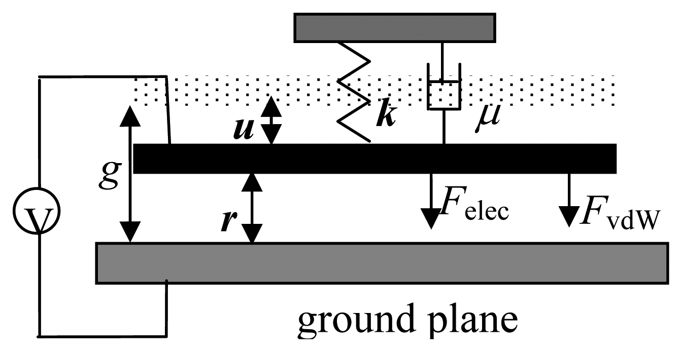
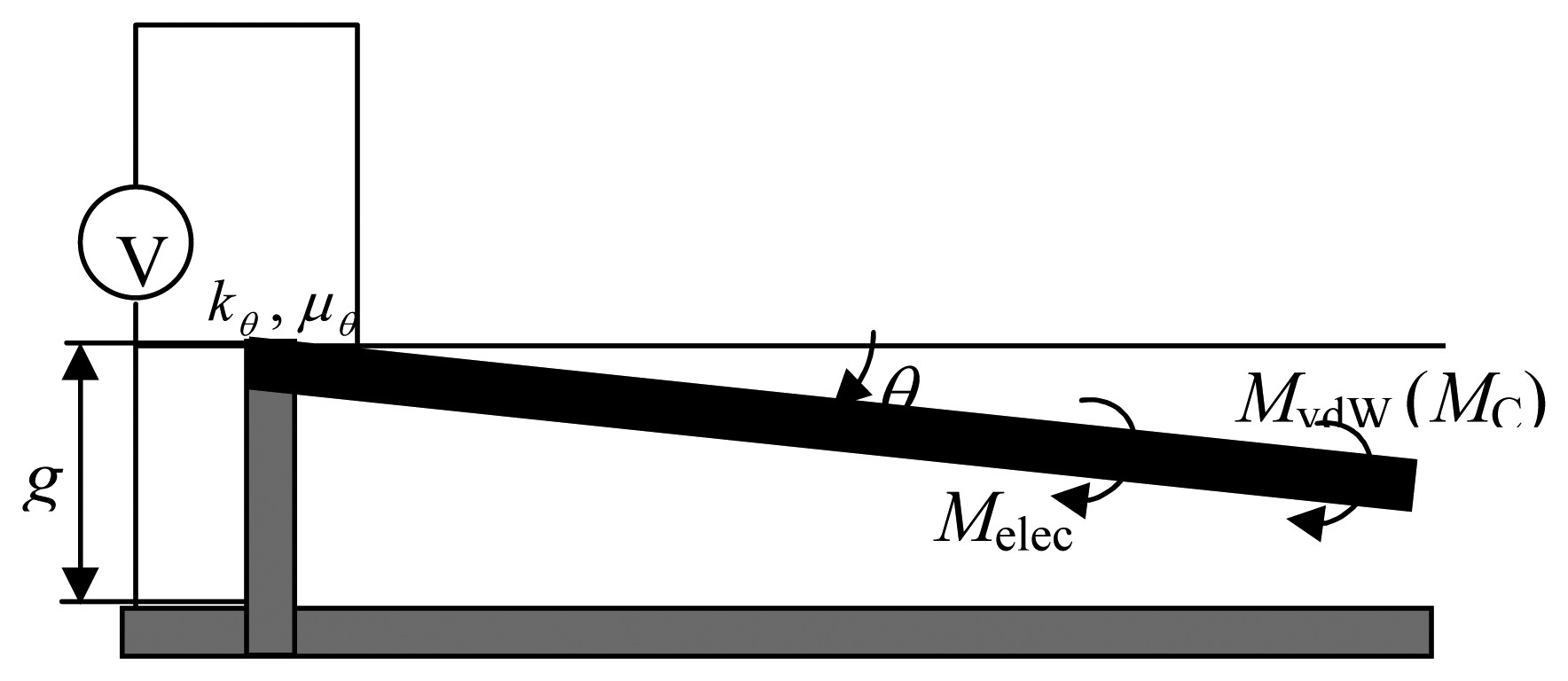
A typical MEM (NEM) parallel-plate (or torsional) actuator is made up of two conducting electrodes, one is typically fixed and the other, which is controlled by an equivalent mechanical spring, is movable (or rotary) [1-4]. The corresponding system can be simplified to one degree of freedom (1DOF). The 1DOF is the displacement,u, of the upper movable beam for the parallel-plate model, and is the torsional angle, θ, for the torsional model. At a certain voltage, the movable electrode becomes unstable and collapses (or pulls-in) to the ground plane. The voltage and displacement (or torsional angle) of the actuators under this state are said to be the pull-in voltage and pull-in displacement (or the pull-in angle) for the parallel-plate (or torsional) actuators, respectively. They are briefly described as the pull-in parameters.
Using a one-dimensional (1D) model, the pull-in parameters have been analytically obtained by many researchers when electrostatic [5-7], vdW and Casimir forces [8-16] are considered. The bifurcation analysis for an electrostatic micro-(nano-) actuator has been addressed in [9-17] with the consideration of electrostatic, vdW, and Casimir forces for the parallel-plate and torsional actuators. In [9, 11, 12], the influences of vdW or Casimir force (torque) on the electrostatic parallel-plate (torsional) actuators was studied. There are two bifurcation points, of which one is a Hopf bifurcation point, and the other is an unstable saddle point. The phase portraits are also drawn, in which periodic orbits are around the Hopf bifurcation point, but the periodic orbit will break into a homoclinic orbit when meeting the unstable saddle point.
In this paper, the influence of damping on the dynamical behavior of the electrostatic parallel-plate and torsional actuators with the vdW or Casimir force (torque) is presented, and the results are compared with those in Refs. [9, 11, 12]. The damping considered in this paper can be a kind of gas (squeeze film) friction which is assumed, without loss of generality, to be linearly proportional to the velocity.

2. System models and dimensionless equations

In this paper, we will use a 1D lumped model (1DLM) to discuss the influence of damping on the dynamical behavior of the parallel-plate and torsional models with electrostatic, vdW and Casimir forces. Then, as in previously published papers [9, 11, 12], MEM (NEM) actuators can be simplified into a 1DOF for these two models. The 1DOF is the displacement, u, of the upper movable beam for the parallel-plate model, and is the torsional angle, θ, for the torsional model. Here, two intermolecular forces, the non-retarded vdW and retarded Casimir, are considered. For convenience, the dimensionless equations are introduced.

2.1. Parallel-plate model

For the parallel-plate model with damping, the system can be simplified to a 1DOF as shown in Figure 1. The 1DOF is the displacement, u, of the upper movable beam, or the gap distance, r. They satisfy the simple geometrical relation: u=gr where g is the initial gap distance between the upper movable beam and the ground plate.
The system is a typical mass-spring-damping one. For the different intermolecular forces, the applied forces on the same model are the electrostatic, vdW, or Casimir forces. Then the equation of motion is
m d 2 u d t 2 + μ d u d t + k u = F elec + F vdW ,
when the vdW force is considered, or
m d 2 u d t 2 + μ d u d t + k u = F elec + F C ,
when the Casimir force is considered. Here, m is the mass of the upper movable beam, μ is the damping coefficient for the parallel-plate model, and k is the spring constant [9, 11].
The electrostatic force Felec (neglecting the fringing force) acting between the planes with potential difference V, the vdW force FvdW and the retarded Casimir force, respectively, are
F elec = ε 0 w L V 2 2 ( g u ) 2 , F vdW = AwL 6 π 1 ( g u ) 3 , F C = π 2 cwL 240 ( g u ) 4 ,
where ε0 is the permittivity of vacuum within the gap, A= π22 is the Hamaker constant which lies in the range (0.4–4)10−19 J, ρ is the volume density of graphite, C is a constant charactering the interactions between the two atoms, ħ is Planck's constant divided by 2π, and is equal to 1.055×10⁻³⁴ Js, c is the speed of light and is equal to 2.988×10⁸ms-1. L and w are the length and width of the upper movable beam, respectively.
Introducing dimensionless variables: Δ =u/g, τ =t/T, μ̄=μ/kT, a= ε0wLV2/2kg3, bvdW =AwL/6πkg4, bc= π2ħcwL/240kg5, and characteristic time T = m / k. Equations (1) and (2) can be transformed into a dimensionless form:
d 2 Δ d τ 2 + μ ¯ d Δ d τ + Δ = a ( 1 Δ ) 2 + b vdW ( 1 Δ ) 3 ,
when the vdW force is considered, or
d 2 Δ d τ 2 + μ ¯ d Δ d τ + Δ = a ( 1 Δ ) 2 + b C ( 1 Δ ) 4 ,
when the Casimir force is considered.
According to the definition of these parameters, physically meaningful solutions exist in the region 0 < Δ < 1. The dimensionless parameter a denotes the order of magnitude of ratio between the electrostatic and elastic forces, bvdW denotes the order of magnitude of ratio between the vdW and elastic forces, bC denotes the order of magnitude of ratio between the Casimir and elastic forces.

2.2. Torsional model

For the torsional structure, the simplified 1DLM is shown in Figure 2.
The 1DOF is the torsional angle, θ. Similar as the parallel-plate model, the equation of motion is:
J d 2 θ d t 2 + μ θ d θ d t + k θ θ = M elec + M vdW ,
when the vdW torque is considered, or
J d 2 θ d t 2 + μ θ d θ d t + k θ θ = M elec + M C ,
when the Casimir torque is considered. Here, J = mL2 /3 is the rotational inertia of the upper rotational beam when the mass is uniformly distributed, kθ is the spring torque coefficient [3], μθ is the damping torque coefficient. According to Ref. [12], the electrostatic torque is
M elec ( θ ) = ε 0 w V 2 2 θ 2 [ ln ( g L θ g ) + L θ g L θ ] ,
the vdW and the Casimir torques, respectively, are
M vdW ( θ ) = A w L 2 12 π g 1 ( g L θ ) 2 , M C ( θ ) = π 2 c w L 2 1440 g 2 3 g L θ ( g L θ ) 3 .
Introducing dimensionless variables: Θ =θ/θmax, Υ =t/Tθ, μ̄Θ=μθ/kθTθ, aΘ=ε0wL3V2/2kθg3, b Θ vdW = A w L 3 / 12 π k θ g 4, b Θ C = π 2 c w L 3 / 1440 k θ g 5, and the characteristic time T θ = J / k θ, equations (5) and (6) can be transformed into the dimensionless form as follows:
d 2 Θ d υ 2 + μ ¯ Θ d Θ d υ + Θ = a Θ Θ 2 [ ln ( 1 Θ ) + Θ 1 Θ ] + b Θ vdW 1 Θ 2 ,
when the vdW torque is considered, or:
d 2 Δ d τ 2 + μ ¯ d Δ d τ + Δ = a ( 1 Δ ) 2 + b C ( 1 Δ ) 4 ,
when the Casimir torque is considered.
According to the definition of these parameters, physically meaningful solutions exist in the region 0 < Θ < 1. The dimensionless parameter aΘ denotes the order of magnitude of ratio between the electrostatic and elastic torques, b Θ vdW denotes the order of magnitude of ratio between the vdW and elastic torques b Θ C denotes the order of magnitude of ratio between the Casimir and elastic torque.
In the following sections, the four dimensionless equations (3), (4), (7) and (8) will be used to discuss the stability of stationary equilibrium and the dynamical behavior for the two different models as referred before. For each model, we will discuss three different cases, according to the different forces applied on the actuators. First, we just consider the electrostatic force (or torque); secondly, we consider the electrostatic and vdW forces (or torques); and last, we consider the electrostatic and Casimir forces (or torques).

3. Pull-in parameters

In this section, we discuss the stability of the stationary equilibrium of the above equations, then we should set zero the velocity and acceleration for each model.

3.1. Parallel-plate model

Case I: just with electrostatic force

In this part, we just consider the electrostatic force and the corresponding equation from equations (3) or (4) is
d 2 Δ d τ 2 + μ ¯ d Δ d τ + Δ = a ( 1 Δ ) 2 .
Setting, d2Δ/dτ2= 0, dΔ/dτ=0 we get the following equation to obtain the stationary equilibrium solution:
f ( Δ , a ) = ( 1 Δ ) 2 Δ a = 0 .
According to the critical condition δf(Δ)/δΔ=0[18] and equation (10), we get
Δ PI = 1 3 , a PI = ε 0 w L V PI 2 2 k g 3 = 4 27 .

Case II: with electrostatic and vdW forces

For this case, using the same procedure as Case I and using equation (3), we get the pull-in parameters as follows:
{ ( 3 Δ PI 1 ) ( 1 Δ PI ) 3 + b vdW = 0 , a PI = ( 4 Δ PI 1 ( 1 Δ PI ) 2 .
The variation of the pull-in parameters ΔPI and aPI with bvdW are plotted in Figures 3 and 4 by equation (12). In these two figures, we notice two special points. The point “°” corresponds to ( b o vdW , Δ o ) = ( 0 , 1 / 3 ) in figure 3, and ( b o vdW , a o ) = ( 0 , 4 / 27 ) in Figure 4. The second point “*” corresponds to ( b * vdW , Δ * ) = ( 27 , 256 , 1 / 4 ) in Figure 3, and ( b * vdW , a * ) = ( 27 / 256 , 0 ) in Figure 4.

Case III: with electrostatic and Casimir forces

Similarly, by using the equation (4), we get the two pull-in parameters with Casimir force as:
{ ( 3 Δ PI 1 ) ( 1 Δ PI ) 4 + 2 b C = 0 , a PI = 1 2 ( 5 Δ PI 1 ( 1 Δ PI ) 2 .
The variations of the pull-in parameters ΔPI and aPI with bC are plotted in Figures 3 and 4, respectively, by equation (13). Two special points are also noticed. The point “°” is the same as in Case II. The point “*” corresponds to ( b * C , Δ * ) = ( 256 / 3125 , 1 / 5 ) in Figure 3, and ( b * C , a * ) = ( 256 / 31251 , 0 ) in Figure 4.
At the point “°”, it implies that there is no vdW or Casimir force on the structure. The results are consistent with those in equation (11). With increasing of the vdW or Casimir force, the pull-in parameters decrease. Until b > b * vdW ( o r b * C ), a is negative. It implies the structure will lose its stability even though there is no voltage applied at the parallel-plate structure.

3.2. Torsional model

Case I: just with electrostatic torque

The governing equation for the system just subjected to the electrostatic force is:
d 2 Θ d υ 2 + μ ¯ θ d Θ d υ + Θ = a Θ Θ 2 [ ln ( 1 Θ ) + Θ 1 Θ ] ,
by setting zero the b Θ vdW or b Θ C in equations (7) or (8).
To get the pull-in parameters, we also set d2Θ/dΥ2=0, dΘ/dΥ=0. As Ref. [12], we obtain the pull-in parameters as:
Θ PI = 0.4404 , a Θ PI = 0.4137 .

Case II: with electrostatic and vdW torques

Using equation (7), we obtain the two critical equations:
{ ( 1 Θ PI ) [ 3 Θ PI ( 1 Θ PI ) 3 2 b Θ vdW ] [ ln ( 1 Θ PI ) + Θ PI 1 Θ PI ] = Θ PI 2 [ Θ PI ( 1 Θ PI ) 2 b Θ vdW ] , a Θ PI = Θ PI 2 Θ PI b Θ vdW ( 1 Θ PI ) 2 ln ( 1 Θ PI ) + Θ PI 1 Θ PI .
The variations of the pull-in parameters θPI and aθPI with b Θ vdW are plotted by equation (15) in Figures 5 and 6, respectively. The point “°” corresponds to ( b Θ o vdW , Θ o ) = ( 0 , 0.4404 ) in Figure 5, and ( b Θ o vdW , a Θ o ) = ( 0 , 0.4137 ) in Figure 6. The point “*” corresponds to ( b Θ * vdW , Θ * ) = ( 4 / 27 , 1 / 3 ) in Figure 5, and ( b Θ * vdW , a Θ * ) = ( 4 / 27 , 0 ) in Figure 6.

Case III: with electrostatic and Casimir torques

Similarly by equation (8), we obtain the pull-in parameters as:
{ 3 ( 1 Θ PI ) [ Θ PI ( 1 Θ PI ) 4 2 b Θ C ] [ ln ( 1 Θ PI ) + Θ PI 1 Θ PI ] = Θ PI 2 [ Θ PI ( 1 Θ PI ) 3 b Θ C ( 3 Θ PI ] , a Θ PI = Θ PI 2 Θ PI b Θ C 3 Θ PI ( 1 Θ PI ) 3 ln ( 1 Θ PI ) + Θ PI 1 Θ PI .
The variations of the pull-in parameters ΘPI and aΘPI with b Θ C are plotted by equation (16) in Figures 5 and 6, respectively. The point “°” is same as in Case II. The point “*” corresponds to ( b Θ * C , Θ * ) = ( 0.0385 , 0.2679 ) in Figure 5, and ( b Θ * C , a Θ * ) = ( 0.0385 , 0 ) in Figure 6.
At the point “°”, it implies that there is no vdW or Casimir torque on the structure. These results are consistent with those in equation (14). The pull-in parameters decrease with increasing vdW or Casimir torque. Until b > b Θ * vdW ( o r b Θ * C ), a is negative. It implies the structure will lose its stability even though there is no voltage applied at the parallel-plate structure.

4. Dynamical behavior

In this section, we just discuss the dynamical behavior of the parallel-plate model with the electrostatic and vdW forces.
To discuss the dynamical behavior of equation (3), first we transform the second-order ordinary differential equation (ODE) (3) into the first-order ODE. Then we set x = Δ, y = dΔ/dτ and obtain:
{ d x d τ = y , d y d τ = μ ¯ y x + a ( 1 x ) 2 + b vdW ( 1 x ) 3 μ ¯ y + f ( x , a , b vdW ) .
The stationary solutions of this system can be obtained by setting zero of the right-hand side of equation (17). From the first equation of (17), we easily get y = 0 Substituting y = 0 into the second equation of (17), we obtain an equivalent function:
x ( 1 x ) 3 + a ( 1 x ) + b vdW = 0 ,
to solve 
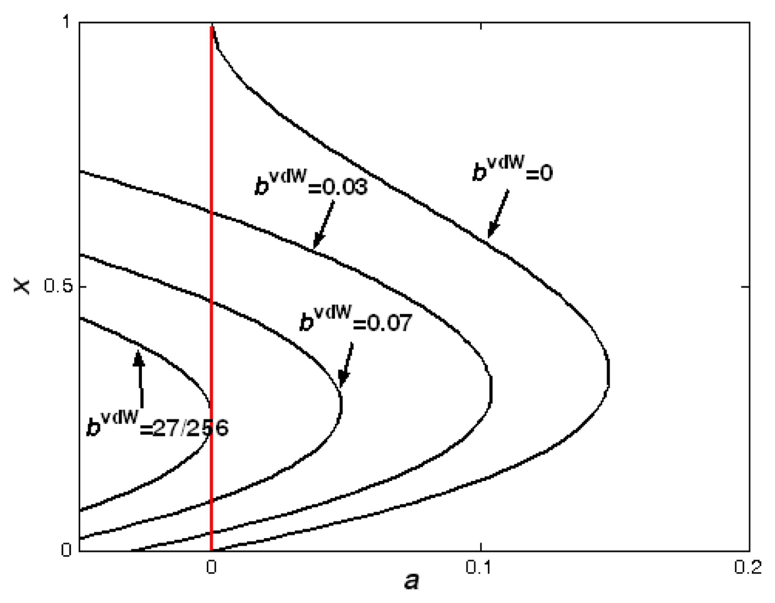
x. The critical condition of this equation has solved in Section 2.1. Now, in order to see clearly the variation of the equilibrium point x with the continuous change of parameters a and bvdW, we solve equation (18) numerically for x as a function of a and bvdW. We plot the variation of x with parameter a for different parameter bvdW, the solution is shown in Figure 7. Because a = ε0wLV2/2kg3 is positive, then the solution is physical meaningful when the solution curves are on the right of a = 0. So from this figure, we notice that equation (18) has one or two equilibrium points for a ≥ 0 just when 0 < b vdW < b * vdW, otherwise there is no equilibrium point.
In order to check the stability of the equilibrium points, we need the Jacobian matrix of equation (17):
J = [ 0 1 f ( x , a , b vdW x μ ¯ ] .
We first discuss the stability of the equilibrium points with the given parameters a = 0 and 0 < b vdW < b * vdW. According to Figure 7, there are two equilibrium points (x1,0)and (x2,0) satisfying the inequality x1< x*<x2.
Firstly, we consider the equilibrium point stability of the special state that there is no electrostatic force on the upper movable beam. Then substituting a = 0 , b vdW < b * vdW and x = x1 < x* into equation (19), we get:
J | x = x 1 = [ 0 1 3 b vdW ( 1 x 1 ) 4 1 μ ¯ ] .
Its corresponding eigenvalues are
λ 1 , 2 = μ ¯ ± μ ¯ 2 + 12 b vbW ( 1 x 1 ) 4 4 2 .
Here, we discuss the property of the eigenvalues when the damping coefficient is positive. Because x1< x*, then 12 b vdW ( 1 x 1 ) 4 4 is absolutely negative. When μ ¯ 2 + 12 b vdW ( 1 x 1 ) 4 4 > 0, the two eigenvalues λ1,2 are all real, and they all are absolutely negative. This means the equilibrium point (x1,0) is a stable node. According to the property of node, this point is an equilibrium point at first. At this position, the elastic force is equal to the vdW force, and the parallel-plate actuator keeps balance state. When we add a small perturbation on the upper movable beam, the perturbation will die out at the stable node. When μ ¯ 2 + 12 b vdW ( 1 x 1 ) 4 4 < 0, the two eigenvalues λ1,2 are a pair of complex conjugates, and the real parts of them are absolutely negative. This means the equilibrium point (x1,0) is a stable focus. According to the property of focus, this point is also an equilibrium point at first. When we add a small perturbation on the upper movable beam, then the trajectory close to the equilibrium position resembles a spiral. Above all, at the point of (x1,0), the real parts of the eigenvalues are negative, this equilibrium point (x1,0) is always stable. Subsequently, we take a = 0 , b vdW < b * vdW and x = x2 > x* into equation (19), solve its eigenvalue equation, we know that it has two real roots, of which one is positive, the other is negative. This means that the equilibrium point (x2,0) is a saddle point. At equilibrium position, if we add a small perturbation on it, the trajectory of the upper movable beam will leave the equilibrium position because one of the eigenvalues is positive. We then call this equilibrium state unstable.
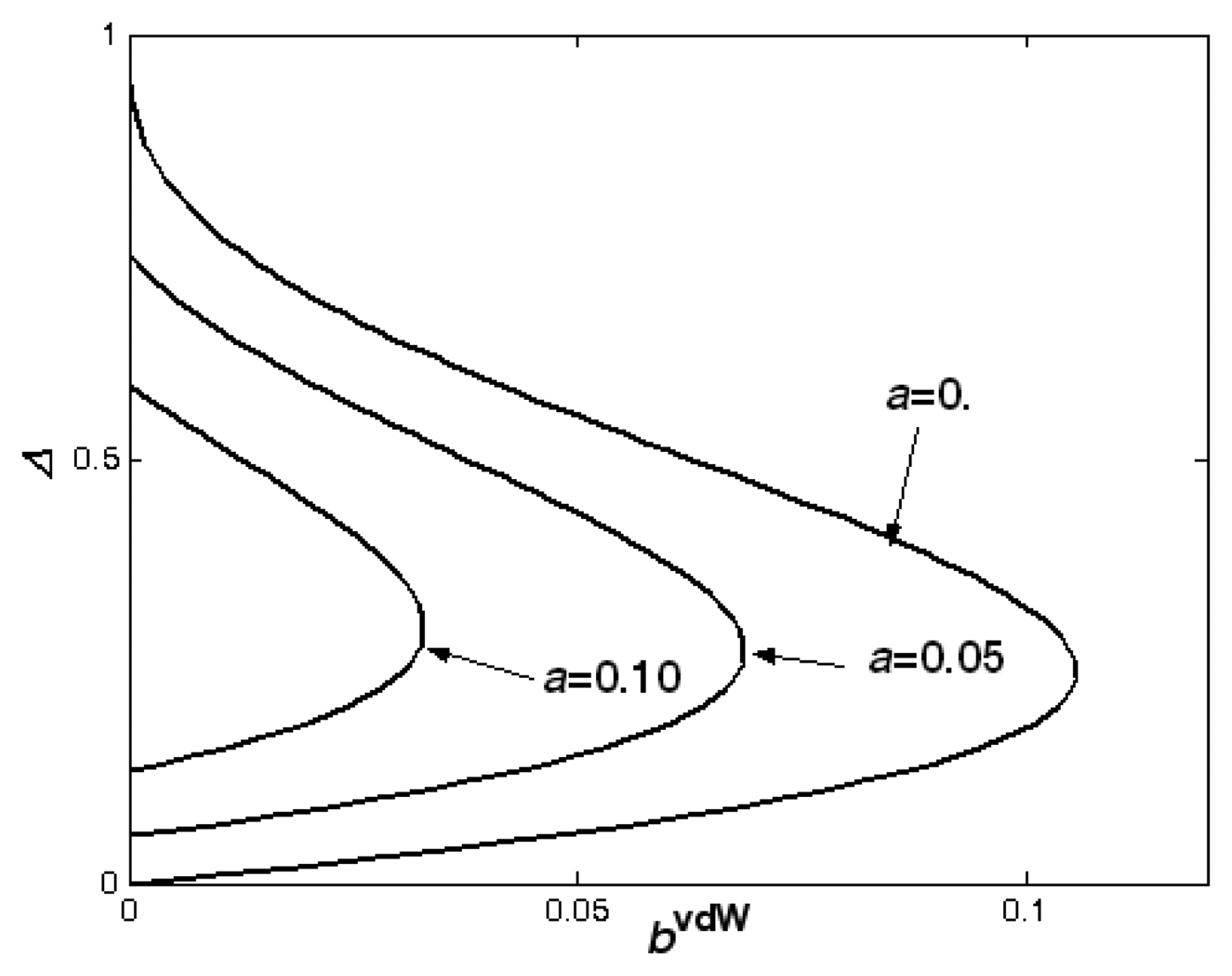
Secondly, applying the same method to discuss the stability of the two solutions with any different given a and bvdW, we plot the bifurcation diagram as Figure 8. In Figure 8, all the points of the lower branch represent the stable points, and all the points of the upper branch are the unstable saddle points, the upper beam is unstable.
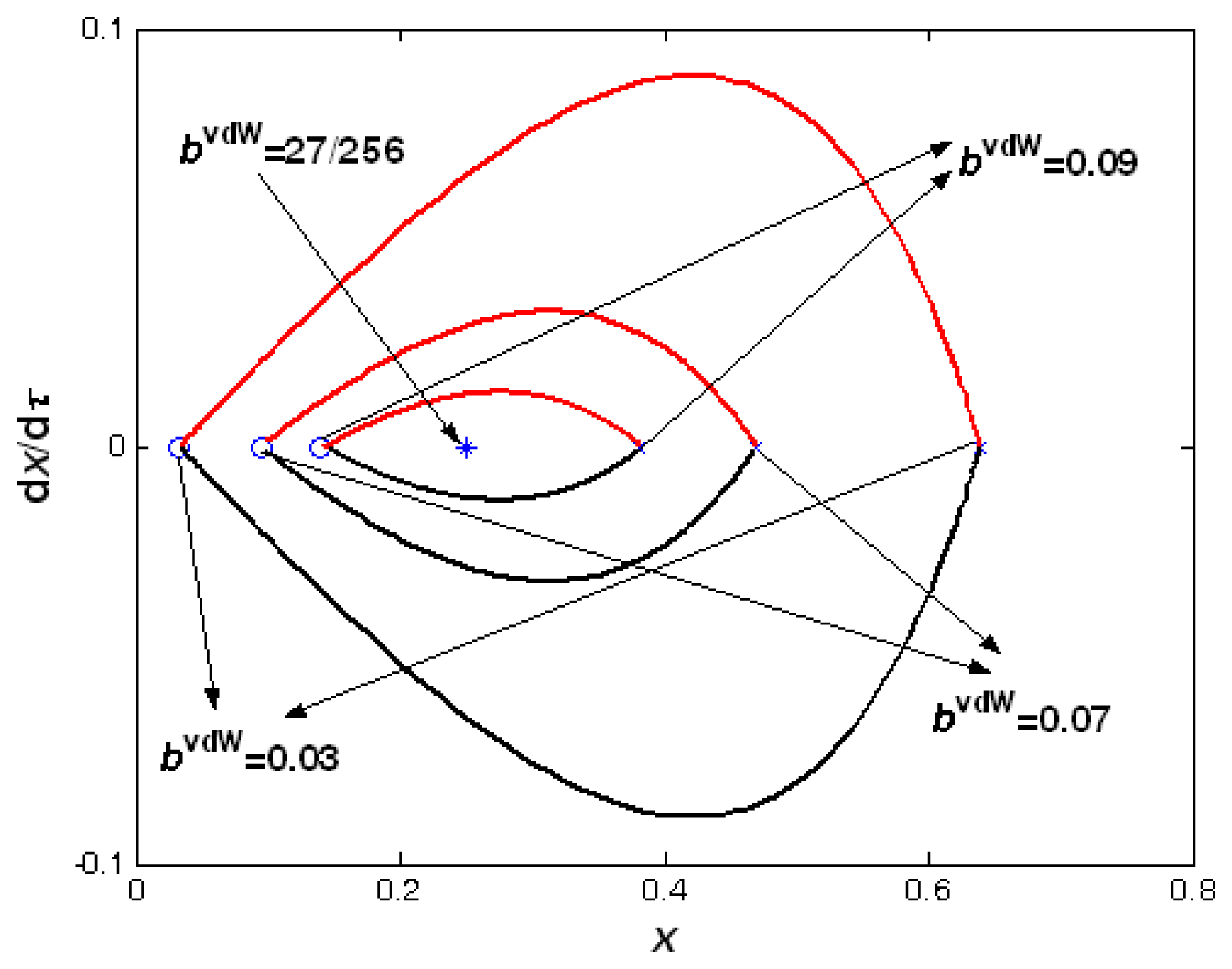
According to the properties of the stable node, stable focus, and saddle point, there exist two heteroclinic orbits which depart from the unstable saddle point and be end at the stable point. In order to see the movement process of the equilibrium points, we draw the phase portraits with a = 0 by setting parameter bvdW equal to 0.03, 0.07 and 0.09, respectively. These phase portraits are shown in Figures 9, 10, 11 and 12. From the discussion in the paragraph above, one knows that the ability of the stable point is different with the variation of damping coefficient μ̄
In Figure 9, we set μ̄ = 3. This value of μ̄ makes sure that μ ¯ 2 + 12 b vdW ( 1 x 1 ) 4 4 > 0 for three different bvdW. By observing Figure 9, there are two equilibrium points for three different 
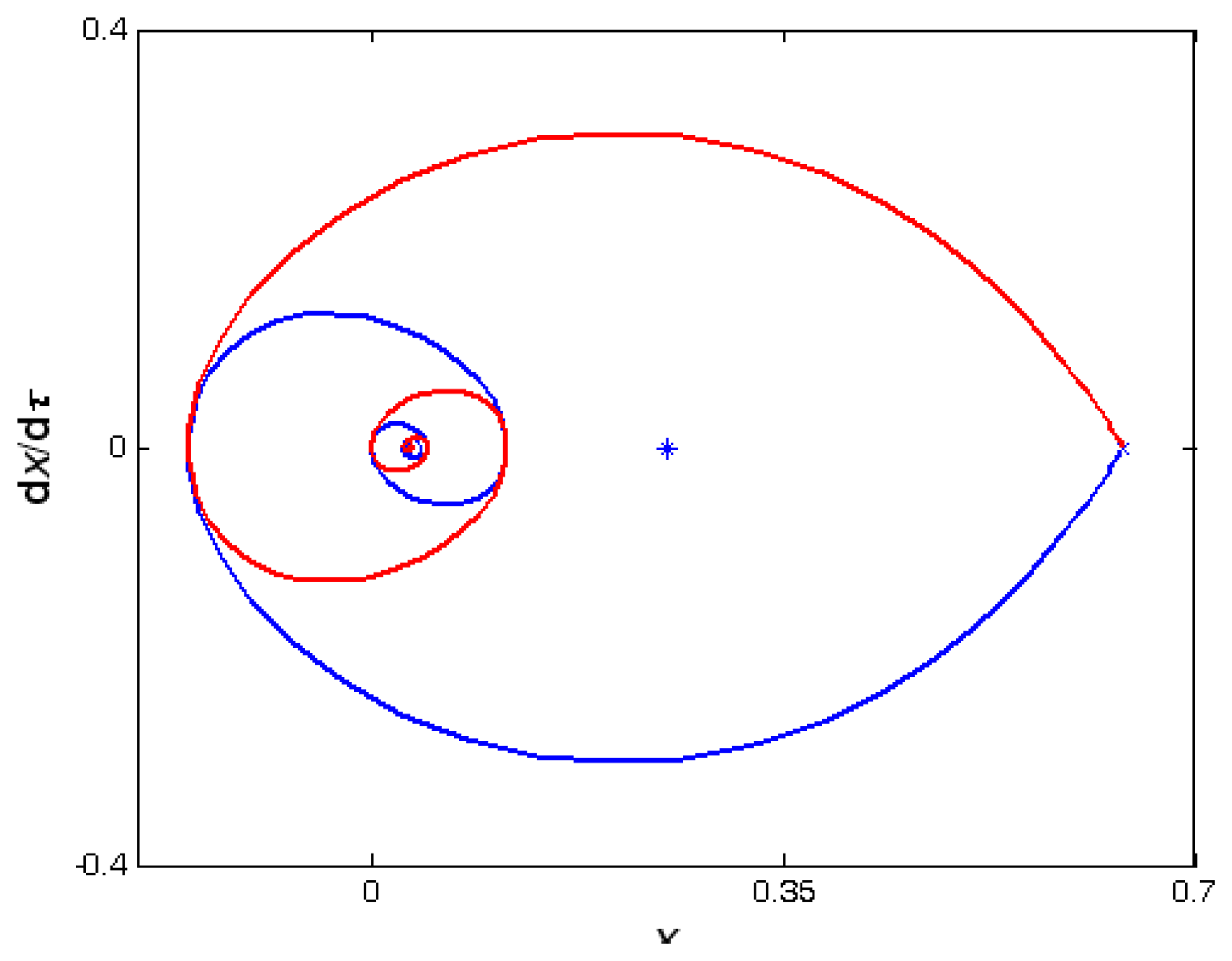
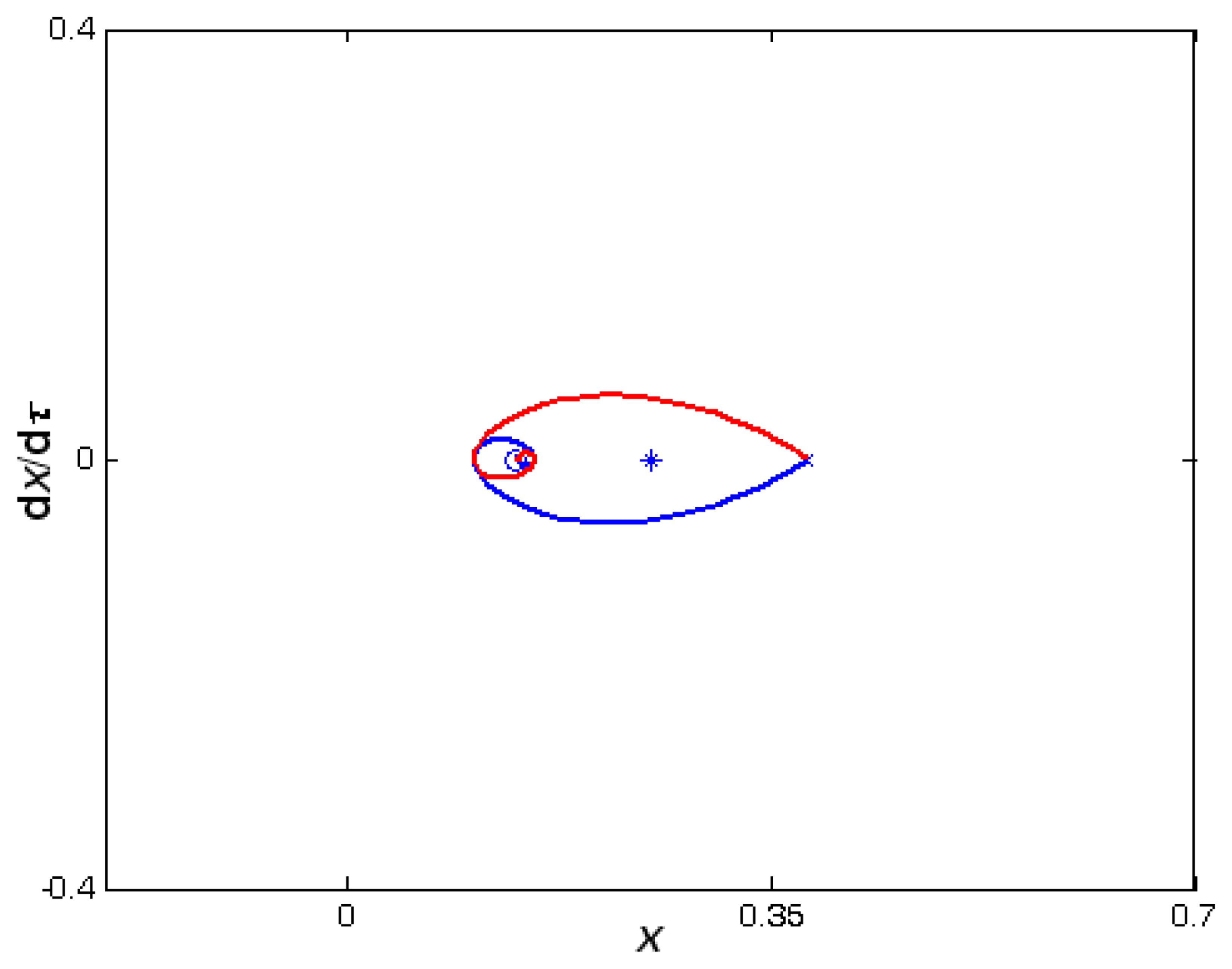
bvdW, one is the stable node (marked by “°”), and the other is the unstable saddle point (marked by “×”). There are two heteroclinic orbits between the unstable saddle point and the stable node. We note that the heteroclinic orbit is convergent to the stable node from the unstable saddle point with exponent. In Figures 10-12, we set μ̄ = 0.5. This value of μ̄ makes sure that μ ¯ 2 + 12 b vdW ( 1 x 1 ) 4 4 < 0 for three different bvdW. By observing Figures 10-12, there are also two equilibrium points for three different bvdW, one is the stable focus (marked by “°”), and the other is the unstable saddle point (marked by “×”). There are two heteroclinic orbits between the unstable saddle point and the stable node. We note that the heteroclinic orbit is convergent to the stable focus from the unstable saddle point spirally, which is different from the stable node because of the difference of their eigenvalues.
From these four figures, we also note that the stable point which is node or focus, and unstable saddle point move to the point “*” from opposite direction with bvdW is increasing. These two points turn into the pull-in point ( x * , d x * / d τ ) = ( 1 / 4 , 0 ) with b * vdW = 27 / 256. At this critical condition, the pull-in phenomenon occurs, the reason of structure invalidation is that the original two equilibrium points merge as one with the changing of parameter bvdW.
According to the eigenvalue equation (20), at least the real part of one of eigenvalues λ1, λ2 is positive when the damping coefficient is negative. At this time, the system is unstable, which should be avoided in engineering applications.
Until now, the dynamical behavior of equation (3) is thoroughly discussed, that is, the dynamical behavior of the parallel-plate model with the electrostatic and vdW forces. For equations (4), (7), and (8), their dynamic behavior can be discussed similarly to equation (3).

5. Discussion and Conclusions

The influence of damping on the dynamical behavior of the electrostatic parallel-plate and torsional actuators with the vdW or Casimir force (torque) is presented. First, we studied the variation of two pull-in parameters with another parameter with different surface forces (torques), we get two special points for each case shown in Figures 3-6. The first special point plotted by “°” shows that the vdW or Casimir force (torque) is zero on the actuator. The second point plotted by “*” illustrates the actuator will lose its stability even though there is no applied voltage. With the appearance the vdW or Casimir force (torque), the pull-in parameters are all decreasing. From Figures 3-6, we also know that the influence of Casimir force (torque) is stronger than that of vdW force (torque) for the same parallel-plate (torsional) actuators with the same geometrical parameters. This result is the same as [9, 11, 12]. Then we can conclude that the damping does not affect the number of equilibrium points.
Secondly, we studied the stability of equilibrium points. One equilibrium point is an unstable saddle with different damping coefficient, the other is a stable node when damping coefficient is greater than some critical value, and otherwise it is a stable focus. Then there are two heteroclinic orbits passing from the unstable saddle point to the stable node or focus. Compared with the results in [9, 11, 12], we find that the Hopf bifurcation point is changed into the stable node or focus with different damping coefficient with the appearance of damping, the unstable saddle point is still the same.
As a matter of fact, there are numerous possible sources of dissipation and damping in NEM actuators, which may broadly be classified as either intrinsic or extrinsic. Extrinsic dissipation or damping, such as gas (squeeze film) friction, clamping loss and surface loss, results from interaction of the actuator microstructure with the environment; whereas intrinsic dissipation or damping, such as thermoelastic relaxation, phonon-phonon and phonon-electron interaction, results from properties of the resonating material. The dissipation and damping mechanisms in NEM actuators are quite complicated [19]. This paper only considered the simplest case of damping in the NEM actuators. To gain a better understanding of the dynamic behavior of nano-resonators, more studies are needed on the dissipation or damping mechanisms and their roles in attenuation of the vibration.

Acknowledgments

WHL was supported by the National Natural Science Foundation of China (Grant No. 10602062) and YPZ was supported by the National Basic Research Program of China (973 Program, Grant No. 2007CB310500) and National High-tech R&D Program of China (863 Program, Grant No. 2007AA04Z348).

References

  1. Batra, R.C.; Porfiri, M.; Spinello, D. Review of modeling electrostatically actuated microelectromechanical systems. Smart Mater. Struct. 2007, 16, R23–R31. [Google Scholar]
  2. Osterberg, P.M. Electrostatically actuated micromechanical test structures for material property measurement. PhD Dissertation, MIT, Cambridge, MA, 1995. [Google Scholar]
  3. Degani, O. Pull-in study of an electrostatic torsion microactuator. J. Microelectromech. Syst. 1998, 7, 373–379. [Google Scholar]
  4. Venkatesh, C.; Pati, S.; Bhat, N.; et al. A torsional MEMS varactor with wide dynamic range and low actuation voltage. Sensor. Actuat. A 2005, 121, 480–487. [Google Scholar]
  5. Bochobza-Degani, O.; Socher, E.; Nemirovsky, Y. On the effect of residual charges on the pull-in parameters of electrostatic actuators. Sensor. Actuat. A 2002, 97-98, 563–568. [Google Scholar]
  6. Pelesko, J.A. Multiple solutions in electrostatic MEMS. Proc. Model. Simul. Microsyst. 2001, 290–293. [Google Scholar]
  7. Bernstein, D.; Guidotti, P.; Pelesko, J.A. Mathematical analysis of an electrostatically actuated MEMS device. Proc. Model. Simul. Microsyst. 2000, 489–492. [Google Scholar]
  8. Dequesnes, M.; Rotkin, S.V.; Aluru, N.R. Calculation of pull-in voltages for carbon-nanotube-based nanoelectromechanical switches. Nanotechnology 2002, 13, 120–131. [Google Scholar]
  9. Lin, W.H.; Zhao, Y.P. Dynamics behavior of nanoscale electrostatic actuators. Chin. Phys. Lett. 2003, 20, 2070–2073. [Google Scholar]
  10. Esquivel-Sirvent, R.; Reyes, L.; Barcenas, J. Stability and the proximity theorem in Casimir actuated nano devices. New J. Phys. 2006, 8, 241–249. [Google Scholar]
  11. Lin, W.H.; Zhao, Y.P. Nonlinear behavior for nanoscales electrostatic actuators with Casimir force. Chaos, Solit. Fract. 2005, 23, 1777–1785. [Google Scholar]
  12. Lin, W.H.; Zhao, Y.P. Stability and bifurcation behavior of electrostatic torsional NEMS varactor influenced by dispersion forces. J. Phys. D: Appl. Phys. 2007, 40, 1649–1654. [Google Scholar]
  13. Guo, J.G.; Zhao, Y.P. Influence of van der Waals and Casimir forces on electrostatic torsional actuators. J. Microelectrom. Syst. 2004, 13, 1027–1035. [Google Scholar]
  14. Palasantzas, G.; DeHosson, J.Th. M. Phase maps of microelectromechanical switches in the presence of electrostatic and Casimir force. Phys. Rev. B 2005, 72, 121409. [Google Scholar]
  15. Palasantzas, G.; DeHosson, J.Th. M. Phase maps of microelectromechanical switches in the presence of Casimir force and finite plasmon frequency corrections. J. Appl. Phys. 2006, 99, 084906. [Google Scholar]
  16. Palasantzas, G.; DeHosson, J.Th. M. Pull-in characteristics of electrostatical switches in the presence of Casimir forces: Influence of self-affine surface roughness. Phys. Rev. B 2005, 72, 115426. [Google Scholar]
  17. Palasantzas, G. Adhesion stability of rough elastic films in presence of quantum vacuum fluctuations. J. Adhes. Sci. Technol. 2006, 20, 1321–1331. [Google Scholar]
  18. Seydel, R. In Practical Bifurcation and Stability Analysis: From Equilibrium to Chaos.; Interdisciplinary Applied Mathematics. Springer-Verlag: Berlin, 1994. [Google Scholar]
  19. Cleland, A.N. Foundations of Nanomechanics; Springer: New York, 2003. [Google Scholar]
Figure 1. 1DLM for the parallel-plate actuator.
Sensors 07 03012f1
Figure 2. 1DLM for the torsional actuator.
Sensors 07 03012f2
Figure 3. Comparison between vdW and Casimir forces with variation of the pull-in displacement ΔPI with parameter b.
Sensors 07 03012f3
Figure 4. Comparison between vdW and Casimir forces with variation of the pull-in parameter aPI with parameter b.
Sensors 07 03012f4
Figure 5. Comparison between vdW and Casimir torques with variation of the pull-in angle ΘPI with parameter bΘ.
Sensors 07 03012f5
Figure 6. Comparison between vdW and Casimir torques with variation of the pull-in parameter aΘPI with parameter bΘ.
Sensors 07 03012f6
Figure 7. Variation of equilibrium points with parameter a for different parameter bvdW with vdW force.
Sensors 07 03012f7
Figure 8. Bifurcation diagram: variation of equilibrium points with parameter bvdW for different a.
Sensors 07 03012f8
Figure 9. Heteroclinic orbits with a = 0 and bvdW 0.03,0.07,0.09, respectively when μ̄ = 3.
Sensors 07 03012f9
Figure 10. Heteroclinic orbits with a = 0 and bvdW = 0.03 when μ̄ = 0.5.
Sensors 07 03012f10
Figure 11. Heteroclinic orbits with a = 0 and bvdW = 0.07 when μ̄ = 0.5.
Sensors 07 03012f11
Figure 12. Heteroclinic orbits with a = 0 and bvdW = 0.09 when μ̄ = 0.5.
Sensors 07 03012f12

