Remote Sensing Sensors and Applications in Environmental Resources Mapping and Modelling


1
Department of Environmental Studies, Florida International University, Miami, Florida, USA
2
Center for Urban and Environmental Change, Department of Geography, Indiana State University
3
International Water Management Institute, Sri Lanka
4
EROS-United States Geological Survey
*
Author to whom correspondence should be addressed.
Sensors 2007, 7(12), 3209-3241; https://doi.org/10.3390/s7123209
Submission received: 8 November 2007
/
Accepted: 26 November 2007
/
Published: 11 November 2007
(This article belongs to the Special Issue Remote Sensing of Natural Resources and the Environment)
Abstract
:The history of remote sensing and development of different sensors for environmental and natural resources mapping and data acquisition is reviewed and reported. Application examples in urban studies, hydrological modeling such as land-cover and floodplain mapping, fractional vegetation cover and impervious surface area mapping, surface energy flux and micro-topography correlation studies is discussed. The review also discusses the use of remotely sensed-based rainfall and potential evapotranspiration for estimating crop water requirement satisfaction index and hence provides early warning information for growers. The review is not an exhaustive application of the remote sensing techniques rather a summary of some important applications in environmental studies and modeling.
1. Overview of remote sensing in environmental studies/modeling
The use of remotely-sensed data in natural resources mapping and as source of input data for environmental processes modeling has been popular in recent years. With the availability of remotely-sensed data from different sensors of various platforms with a wide range of spatiotemporal, radiometric and spectral resolutions has made remote sensing as, perhaps, the best source of data for large scale applications and study. In this review, we summarize some of the most commonly used applications of the technique in environmental resources mapping and modeling. Applications of remote sensing in hydrological modeling, watershed mapping, energy and water flux estimation, fractional vegetation cover, impervious surface area mapping, urban modeling and drought predictions based on soil water index derived from remotely-sensed data is reported. The review also summarizes the different eras of sensors development and remote sensing and future directions of the remote sensing applications.
1.1 Evolution and advances in remote sensing satellites and sensors for the study of environments
There are eight distinct eras of remote sensing; some running parallel in time periods, but are distinctly unique in terms of technology, concept of utilization of data, applications in science, and data characteristics (e.g., Table 1). These are discussed below:
- Airborne remote sensing era: The airborne remote sensing era evolved during the first and the Second World War (Avery and Berlin, 1992, Colwell, 1983). During this time remote sensing was mainly used for the purposes of surveying, reconnaissance, mapping, and military surveillance.
- Rudimentary spaceborne satellite remote sensing era: The spaceborne remote sensing era began with launch of “test of concept” rudimentary satellites such as Sputnik 1 from Russia and Explorer 1 by the United States at the end of 1950s (Devine, 1993, House et al., 1986). This was soon followed by the first meteorological satellite called Television and Infrared Observational Satellite-1 (TIROS-1) by the United States also in the late 1950s (House et al., 1986).
- Spy satellite remote sensing era: During the peak of the cold war, spy satellites such as Corona (Dwayne et al., 1988) were widely used. Data was collected, almost exclusively, for military purposes. The data was not digital, but was produced as hard copies. However, the spin-off of the remote sensing developed for military purposes during the above 3 eras spilled over to mapping and slowly into environmental and natural resources applications.
- Meteorological satellite sensor remote sensing era: The early meteorological satellite sensors consisted of geo-synchronous Geostationary Operational Environmental Satellite (GOES) and polar-orbiting National Oceanic and Atmospheric Administration (NOAA) Advanced Very High Resolution Radiometer (AVHRR) (Kramer, 2002). This was an era when data started being available in digital format and were analyzed using exclusive computer hardware and software. This was also an era when global coverage became realistic and environmental applications practical.
- Landsat era: The Landsat era begins with the launch of Landsat-1 (then called Earth Resources Technology Satellite) in 1972 carrying multi spectral scanner (MSS) sensor. This was followed by other path-finding Landsat satellites 2 through 3 which carried MSS and 4 and 5 which carried Thematic Mapper (TM). The Landsat 7 carries Enhanced Thematic mapper (ETM+) sensor. The Landsat-6 failed during launch. The Landsat-8 carrying Operational Land Imager (OLI) is planned for launch in 2011. The Landsat era also has equally good sun-synchronous Land satellites such as Systeme Pour l'Observation de Ia Terre (SPOT) of France and, Indian Remote Sensing Satellite (IRS) of India (Jensen, 2000). These satellites have high resolution (nominal 2.5-80 meter) and have global coverage potential. At this resolution, only Landsat is currently gathering data with global wall to wall coverage. This is, by far, the most significant era that kick started truly wide environmental application of remote sensing data locally and globally.
- Earth Observing System era: The Earth Observing System (EOS) era (Stoney, 2005, Bailey et al., 2001, Jensen, 2000, Colwell, 1983) began with launch of Terra satellite in 1999 and has brought in the global coverage, frequent repeat coverage, high level of processing (e.g., georectified, at-satellite reflectance), easy and mostly free access to data. The Terra\Aqua satellites carrying sensors such as Moderate Resolution Imaging Spectroradiometer (MODIS) and Measurements of Pollution in the Troposphere (MOPITT) have daily re-visit and various processed data. Applications of sensor data have become wide spread and applications have multiplied. Institutions and individuals who never used remote sensing have begun to take an interest in remote sensing. Also, the availability of the processed data in terms of products such as leaf area index (LAI) and land use\land cover (LULC) have become routine. Currently, MODIS itself has 40+ products. The active spaceborne remote sensing sensors using radar technology also became prominent around this time (and during the Landsat era) launch of European Radar Satellite (ERS), Japanese Earth Resources satellite (JERS), Radarsat,and Advanced Land Observation Satellite (ALOS). The Shuttle Radar Technology Mission (SRTM) was used to gather data for digital elevation.
- New Millennium era: The new millennium era (Bailey et al., 2001) refers to highly advanced “test-of concept” satellites sent into orbit around the same time as EOS era, but the concepts and ideas are different. These are basically satellites and sensors for the next generation. These include Earth Observing-1 carrying the first spaceborne hyperspectral data. The idea of Advanced Land Imager (ALI) as a cheaper, technologically better replacement for Landsat is also very attractive.
- Private industry era: The private industry era began at the end of the last millennium and beginning of this millennium (see Stoney, 2005). This era consists of a number of innovations. First, collection of data in very high resolution (<10 meter). This is typified by IKONOS and Quickbird satellites. Second, a revolutionary means of data collection. This is typified by Rapideye satellite constellation of 5 satellites, having almost daily coverage of any spot on earth at 6.5 meter resolution in 5 spectral bands including a red-edge band. Third, is the introduction of micro satellites, some under disaster monitoring constellation (DMC), which are designed and launched by surrey satellite technology Ltd. for Turkey, Nigeria, China, USGS, UK, and others. Fourth, is the innovation by Google Earth ( http://earth.google.com) in making rapid data access of VHRI for any part of the World through streaming technology that makes it easy for even a non-specialist to zoom and pan remote sensing data.
1.2 Summary of sensors in environmental modeling
A state-of-art of satellite sensors widely used in environmental applications and natural resources management are given in Table 1. These sensors provide data in a wide range of scales (or pixel resolutions), radiometry, band numbers, and band widths and provides distinct advantage of consistency of data, synoptic coverage, global reach, cost per unit area, repeatability, precision, and accuracy. Added to this is the long-time series of archives and pathfinder datasets (e.g., Tucker, 2005, Agbu and James, 1994) that have global coverage. Much of this data is also free and accessible online.
Many applications (e.g., Thenkabail et al., 2006) in environmental monitoring require frequent coverage of the same area. This can be maximized by using data from multiple sensors (Table 1). However, since data from these sensors are acquired in multiple resolution (spatial, spectral, radiometric), multiple bandwidth, and in varying conditions, they need to be harmonized and synthesized before being used (Thenkabail et al., 2004). This will help normalize for sensor characteristics such as pixel sizes, radiometry, spectral domain, and time of acquisitions, as well as for scales. Also, inter-sensor relationships (Thenkabail, 2004) will help establish seamless monitoring of phenomenon across landscape.
2. Urban Mapping Applications
The majority of remote sensing work has been focused on natural environments over the past decades. Applying remote sensing technology to urban areas is relatively new. With the advent of high resolution imagery and more capable techniques, urban remote sensing is rapidly gaining interest in the remote sensing community. Driven by technology advances and societal needs, remote sensing of urban areas has increasing become a new arena of geospatial technology and has applications in all socioeconomic sectors (Weng and Quattrochi, 2006).
Urban landscapes are typically a complex combination of buildings, roads, parking lots, sidewalks, garden, cemetery, soil, water, and so on. Each of the urban component surfaces exhibits a unique radiative, thermal, moisture, and aerodynamic properties, and relates to their surrounding site environment to create the spatial complexity of ecological systems (Oke 1982). To understand the dynamics of patterns and processes and their interactions in heterogeneous landscapes such as urban areas, one must be able to quantify accurately the spatial pattern of the landscape and its temporal changes (Wu et al. 2000). In order to do so, it is necessary: (1) to have a standardized method to define theses component surfaces, and (2) to detect and map them in repetitive and consistent ways, so that a global model of urban morphology may be developed, and monitoring and modeling their changes over time be possible (Ridd 1995).
Remote sensing technology has been widely applied in urban land use, land cover classification, and change detection. However, it is rare that the classification accuracy of greater than 80% can be achieved by using per-pixel classification (so called “hard classification”) algorithms (Mather 1999). The low accuracy of land use/cover (LU/LC) classification in urban areas is largely attributed to the mixed pixel problem, where several types of LU/LC are contained in one pixel. The mixed pixel problem is resulted from the fact that the scale of observation (i.e., pixel resolution) fails to correspond to the spatial characteristics of the target (Mather 1999). Therefore, the “soft”/fuzzy approach of LU/LC classifications has been applied, in which each pixel is assigned a class membership of each LU/LC type rather than a single label (Wang 1990). Nevertheless, as Mather (1999) suggested, either “hard” or “soft” classifications was not an appropriate tool for the analysis of heterogeneous landscapes. Both Ridd (1995) and Mather (1999) maintained that identification/description/quantification, rather than classification, should be applied in order to provide a better understanding of the compositions and processes of heterogeneous landscapes such as urban areas.
Ridd (1995) proposed a major conceptual model for remote sensing analysis of urban landscapes, i.e., the vegetation - impervious surface - soil (V-I-S) model. It assumes that land cover in urban environments is a linear combination of three components, namely, vegetation, impervious surface, and soil. Ridd believed that this model can be applied to spatial-temporal analyses of urban morphology, biophysical, and human systems. While urban land use information may be more useful in socioeconomic and planning applications, biophysical information that can be directly derived from satellite data is more suitable for describing and quantifying urban structures and processes (Ridd 1995). The V-I-S model was developed for Salt Lake City, Utah, but has been tested in other cities (Ward et al. 2000, Madhavan et al. 2001, Setiawan et al. 2006). All of these studies employed the V-I-S model as the conceptual framework to relate urban morphology to medium-resolution satellite imagery, but “hard classification” algorithms were applied. Therefore, the problem of mixed pixels cannot be solved, and the analysis of urban landscapes was still based on “pixels” or “pixel groups”.
Linear spectral mixture analysis (LSMA) is another approach that can be used to handle the mixed pixel problem, besides the fuzzy classification. Instead of using statistical methods, LSMA is based on physically deterministic modeling to unmix the signal measured at a given pixel into its component parts called endmembers (Adams et al. 1986; Boardman 1993; Boardman et al. 1995). Endmembers are recognizable surface materials that have homogenous spectral properties all over the image. LSMA assumes that the spectrum measured by a sensor is a linear combination of the spectra of all components within the pixel (Boardman 1993). Because of its effectiveness in handling spectral mixture problem and ability to provide continuum-based biophysical variables, LSMA has been widely used in: (1) estimation of vegetation cover (Asner and Lobell 2000; McGwire et al. 2000; Small 2001; Weng et al. 2004; Lee and Lathrop 2005), (2) impervious surface estimation and/or urban morphology analysis (Phinn et al. 2002; Wu and Muarry 2003; Rashed et al. 2003; Lu and Weng 2006a, 2006b; Wu et al. 2005), (3) vegetation or land cover classification (Adams et al. 1995; Cochrane and Souza 1998; Aguiar et al. 1999; Lu and Weng 2004), and (4) change detection (Rashed et al. 2005; Powell et al. 2007). However, with a few exceptions, these studies have focused on technical specifics and on the examination of the effectiveness of LSMA. Only a few studies have explicitly adopted the V-I-S model as the conceptual model to explain urban land cover patterns (Phinn et al. 2002; Wu and Murray 2003; Wu et al. 2005; Lu and Weng 2006a, 2006b; Powell et al. 2007), while others implicitly (Rashed et al. 2003, 2005).
Figure 1 shows LULC map of Indianapolis, United States, derived from a Landsat ETM+ image of June 22, 2000. LULC classes were formed by using LSMA derived fractions with a hybrid procedure that combined maximum-likelihood and decision-tree algorithms (Weng et al. 2004).
Impervious surfaces are anthropogenic features through which water cannot infiltrate into the soil, such as roads, driveways, sidewalks, parking lots, rooftops, and so on. In recent years, impervious surface has emerged not only as an indicator of the degree of urbanization, but also a major indicator of urban environmental quality (Arnold and Gibbons, 1996). Various digital remote sensing approaches have been developed to estimate and map impervious surfaces, including mainly: image classification, multiple regression, sub-pixel classification, artificial neural network, classification and regression tree algorithm, and so on. To study further on this topic, please refer to a book by Weng (2007), entitled “Remote Sensing of Impervious Surfaces”. Through review of basic concepts and methodologies, analysis of case studies, and examination of methods for applying up-to-date techniques to impervious surface estimation and mapping, this book may serve undergraduate and graduate students as a textbook, or be used as a reference book for professionals, researchers, and alike in the academics, government, industries, and beyond.
Figure 2 shows impervious surface images of Indianapolis derived from a Terra's ASTER image of June 16, 2001. LSMA and an ANN model (Multi-Layer Perceptron feed forward network with the back-propagation learning algorithm) were employed to estimate the impervious surfaces. The root-mean-square-error of the impervious surface map with the ANN model was 12.3%, and that resulted from LSMA was 13.2%.
3. Hydrological Applications
Since 1972 (launch of the first Earth Resources Technology Satellite, ERTS-1), scientist have used remotely-sensed data from different sensors to characterize, map, analyze and model the state of the land surface and surface processes. With the help of new algorithms, new hydrological information were extracted from remotely-sensed data and used in hydrological and environmental modeling. These new information and hydrological parameters have increased our understanding of the different hydrological processes by helping in quantifying the rate and amount of water and energy fluxes in the environment. The ability of these sensors in providing various spatiotemporal scales data has also increased our capability in looking into one of the challenges of environmental modeling, mismatch between scales of environmental process and available data.
The role of remote sensing in understanding hydrological processes and fluxes across different spatial and temporal scales can be tremendous, if appropriate spatial and temporal resolution remotely-sensed data are available under ranges of bands. With the availability of large volumes of remotely-sensed data, geographical information system (GIS) tools to manipulate, process, store and retrieve such data and efficient computing system, the application of remote sensing to water resources has been increasing in recent years.
The application of remote sensing in water resources research and management mainly lies in one of the three categories: mapping of watersheds and features, indirect hydrological parameter estimation and direct estimation of hydrological variables.
3.1. Mapping of watersheds and hydrologic features
Different sensors aboard airplane or satellites have been used extensively in providing imaging, photographing and mapping information for different purposes. Mapping of wetlands, floodplains, disaster areas, coastal shores, river banks, snow pack, fire damage, drainage basins and others that show the areal extent of a given land feature distinct from others due to the difference in the spectral signature fall under this category. Different studies have used aerial photos, satellite images, lidar and radar data to map and visualize land surfaces for planning, resource mapping, hazard assessment and emergency operations.
Landsat images were used to capture the expansion of a hydrologically-closed lake, Devils Lake, North Dakota. Results of the study are presented below.
3.1.1 Flood Mapping of Devils Lake
Landsat Thematic Mapper (TM) and Enhanced Thematic Mapper Plus (ETM+) images aboard the Landsat-5 and 7 satellites, respectively, for the years 1991- 2003 were used to delineate flooding map and also compute lake surface area. A mosaic of three Landsat scenes (Path/Row: 31/27, 32/26, 32/27) was used to cover the entire study area.
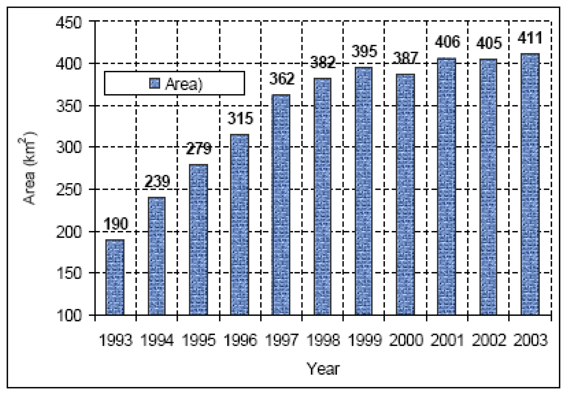
The lake surface area of the chain of Devils Lakes excluding Stump Lake mapped from Landsat for 1993 and 2003 is indicated in Figure 3. Between 1993 and 2003, the surface area of the lake was lowest in 1993 and highest in 2003 (Figures 3).The lake surface area from Landsat images was classified and only lake areas were computed for each respective year. As depicted from the images, the areal increase of the lake is greater in recent years. The white line in Figure 3 marks the lake boundary line in 1992. The corresponding surface areas for 1993 and 2003 are also shown in the figure indicating an increase in the flooded area by 117% between 1993 and 2003.
Figure 4, lake surface area by and year (without Stump Lake) derived from Landsat images, shows that each meter rise of lake inundates a progressively greater area resulting in increased flood volume. It is shown that a 1.3 m increase between 1994 and 1995 at an elevation of 435.8 m adds about 39.5 km2 to the lake's surface area, whereas a 1.3 m increase between 1996 and 1997at an elevation of 438 m adds nearly 49 km2 (Melesse et al. 2006a, 2006b). This indicates the severity of the flooding problem at higher lake levels attributed partly due to the flat topography of the contributing watershed.
3.2. Indirect estimation of Hydrological parameters
The majority of remote sensing contribution in water resources management falls under the indirect hydrological parameter estimation category. The most common area of contribution in this category is the use of classification algorithms to generate land cover classes. Using the unique spectral signature of land surfaces, mainly in the visible, infrared and thermal spectra, land cover classes are estimated from such data.
The use of surface temperature, normalized difference vegetation index (NDVI) and unsupervised classification algorithm is demonstrated in mapping land-cover for the Heart River sub-basin, Missouri River basin in North Dakota.
3.2.1. Land Cover Mapping
Land-cover for the heart River sub-basin of North Dakota was determined from July 2, 2002 Landsat ETM+ image for the study area using ISODATA classification (ERDAS, 1999) (Figure 5a). The unsupervised classifier yielded 30 spectral classes. Scattergram of the scaled Normalized Difference Vegetation Index (NDVIs) versus scaled surface radiant temperature (Ts) were used to find instances of strong correlation between them and the land-cover data of the sub-basin. The spectral signatures of all these classes were used to determine the mean radiance for each band. Using the mean signature values, additional layers and vegetation indices were derived. From the scattergram, five United States Geological Survey Land Use and Land Cover (USGS-LULC) system level 1 land-cover classes (Anderson et al., 1976) were identified (Figure 5b) (Melesse, 2004a).
3.2.2 Fractional Vegetation Cover
To understand the change in the vegetation cover for images of different scenes and dates, the scaled NDVI (NDVIs) has been used by many researchers (Price, 1987; Che and Price, 1992; and Carlson and Arthur, 2000).
Carlson and Ripley (1997) found the relationship between fractional vegetation cover (FVC) and scaled NDVI to be
Where FVC ranges between 0 and 1.
From the 1986 TM and 2000 ETM+ Landsat images, PVC was estimated for Econlockhatchee River sub-basin (Econ sub-basin), Florida and compared to understand the change sin the vegetation cover over the 16 years (Figure 6) (Melesse et al. 2003a, 2003b).
3.3 Impervious surface cover
Surfaces that impede the natural infiltration of water and enhance surface runoff are classified as impervious surfaces. Associated with urbanization and construction of pavements, roads and buildings, impervious surfaces play an important role in surface runoff and the transport of contaminants. Remote sensing has been used as an effective technique to map impervious surfaces using spectral characteristics of surfaces (Melesse 2004b, Melesse and Wang, 2007). Ridd (1995) and Owen et al. (1998) showed that the relation between the fractional vegetation cover (FVC) and fractional impervious surface area (FIS) for developed areas as
In surface runoff estimation, impervious surfaces are classified as hydraulically connected and those that are not. The hydraulically connected surfaces such as parking lots and roads are connected to the drainage system where runoff from such surfaces leads to the drainage network. Those surfaces such as roof-tops are classified as hydraulically not connected. Rain water from roof tops can fall into the pervious surface area such as grass hence termed as disconnected. The resulting storm runoff from such surfaces can be lower than the hydraulically connected impervious surface areas.
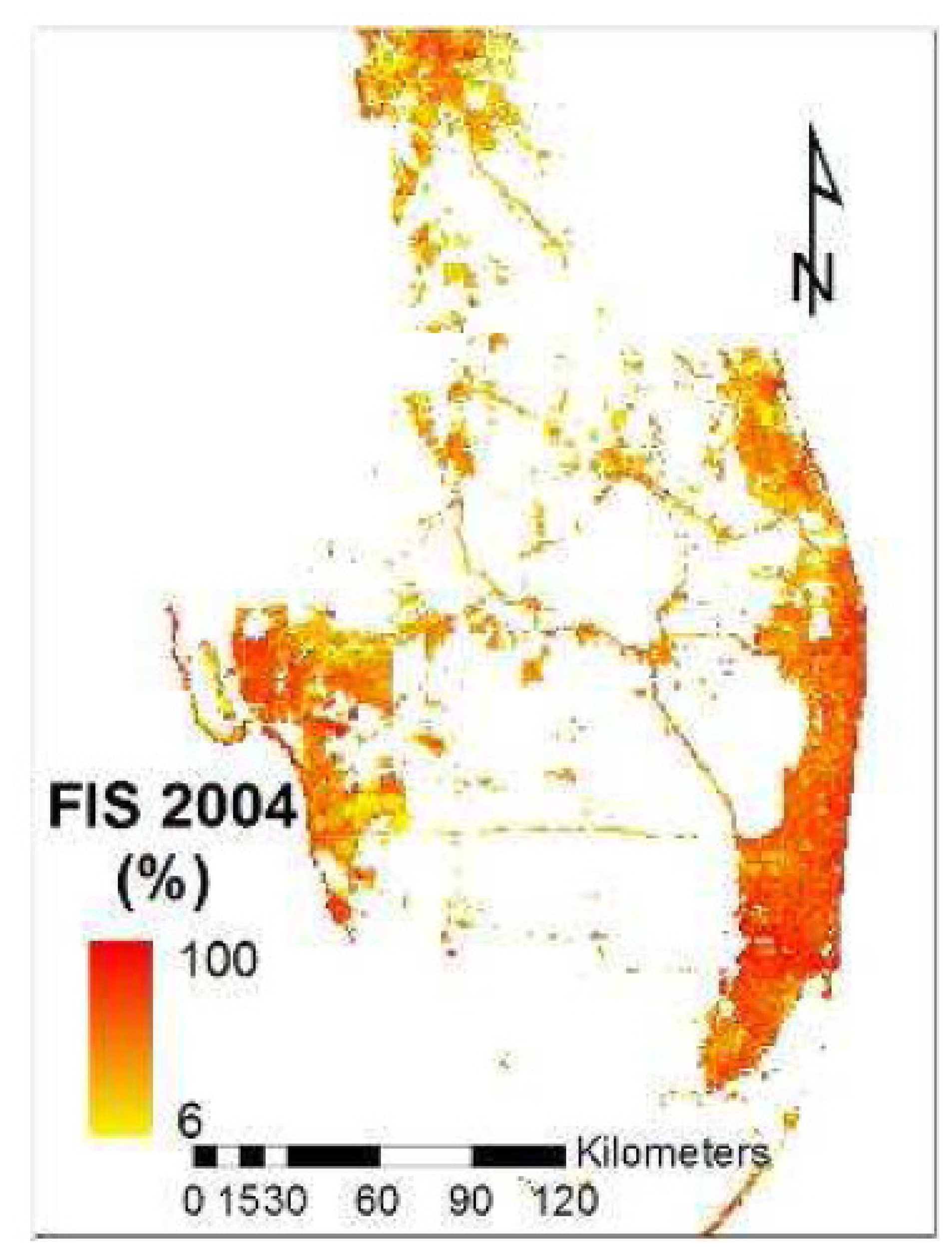
Figure 7 shows the 2004 impervious surface area map of south Florida as estimated from MODIS data using equation (3).
3.4. Micro-topography and latent heat flux
Topography plays an important role in the distribution and flux of water and energy within the natural landscape. Surface runoff, evaporation and infiltration are hydrologic processes that take place at the ground-atmosphere interface. Quantitative assessment of these processes depends on topographic configuration of the landscape, which is one of several controlling boundary conditions.
Wetness index (WI) provides a description of the spatial distribution of the soil moisture using topographic information. WI is computed as,
where A and S are the specific drainage area (flow accumulation) and slope, respectively.
As specific drainage area increases and gradient decreases, WI and soil moisture content increase. Wetness index takes into account both a local slope geometry and site location in the landscape, combining data on gradient and specific drainage area. This can lead to higher correlations of soil moisture with WI, hence evapotranspiration, than with specific drainage area and gradient.
Wetness index controls flow accumulation, soil moisture, distribution of saturation zones, depth of water table, evapotranspiration, thickness of soil horizons, organic matter, pH, silt and sand content, plant cover distribution (Kulagina et al., 1995; Florinsky, 2000).
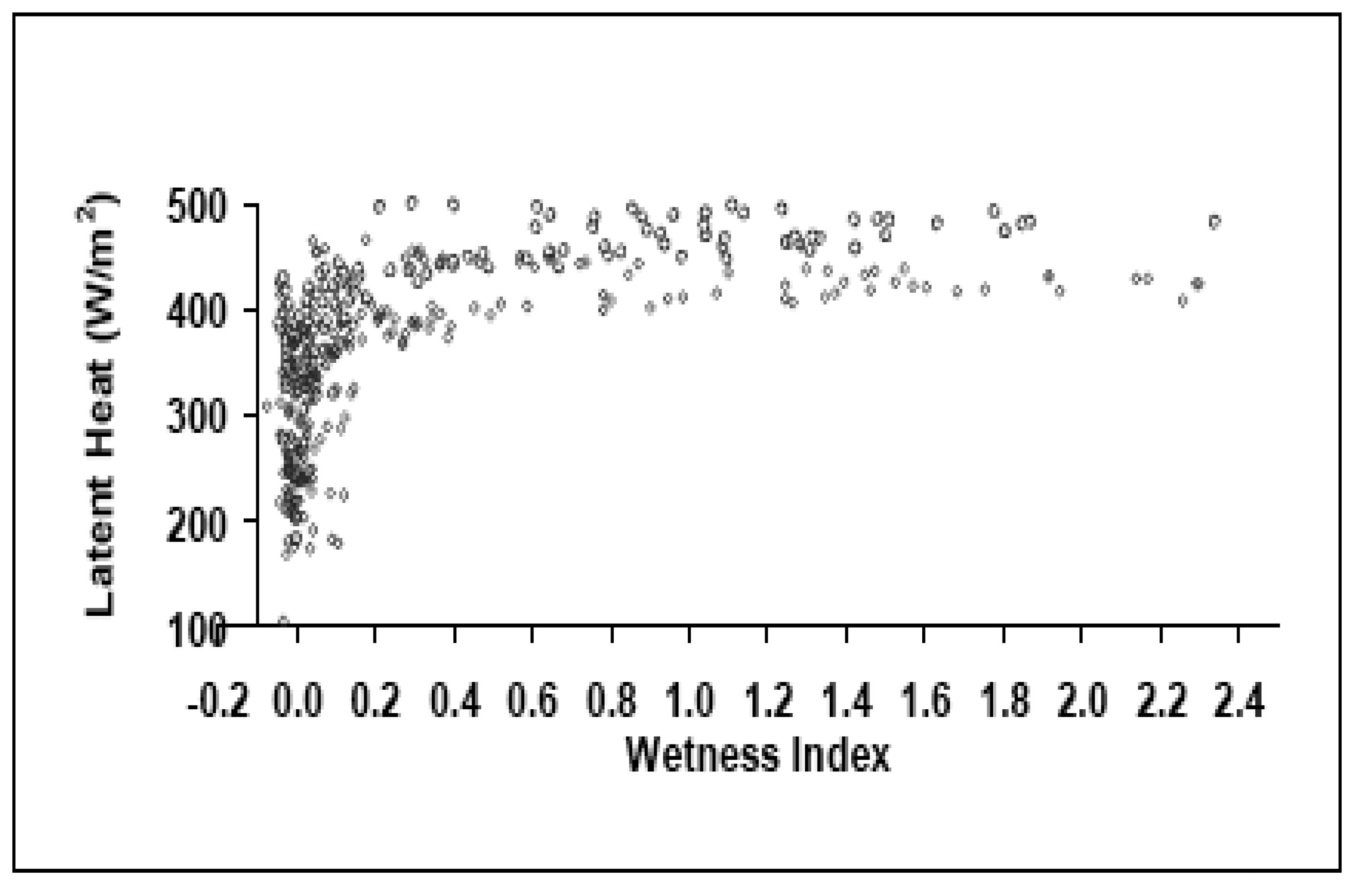
A study to understand the relationship between latent heat flux and microtopography (1m resolution) of a wheat field was studied using remote sensing-based latent heat flux. The latent heat flux estimation technique is based on the surface energy balance approach using remotely-sensed data (Bastiaanssen, 1998). The detailed procedure on estimating grid-based latent heat flux for the study area is shown in Melesse and Nangia (2005) and Oberg and Melesse (2006). The relationship between WI (Figure 8) and latent heat flux for a wheat field is strong, since the topography influences the flux and distribution of water. Grids with higher values of WI are areas receiving most of the flow (higher flow accumulation) and lower gradient. These areas have higher soil moisture, hence higher rate of evaporation, than areas with lower values of WI. It is also indicated that when water is a limiting factor, plants on higher WI areas grow well with good canopy cover than plants in other zones of the field. This increases the transpiration (vegetation latent heat) of the crops. Figure 9 shows the scattergram of WI vs. latent heat. The latent heat seems to increase at higher rate at lower values of WI than at higher values of WI. This is attributed to the limited available water for evaporation proportional to WI.
4. Soil water and drought monitoring for early-warning applications
With the advent of grid-based remotely-sensed rainfall data, the application of crop water balance models for crop monitoring and yield forecasting has gained increased acceptance by various international, national and local organizations around the world. Soil water is a key state variable in hydrological modeling and determines the partitioning of rainfall into runoff and deep percolation, and also controls the rate of evapotranspiration (ET).
Although the estimation of actual evapotranspiration (ETa) is the ultimate goal of many researchers for hydrological and agronomical applications, it is often difficult to quantify and requires expensive instrumentation. However, hydrological modeling techniques are used to estimate ETa. The two basic modeling techniques to estimate ETa are based on either energy balance (e.g., Bastiaanssen et al, 1998; Allen et al, 2005; Senay et al, 2007a) principles or water balance-based algorithms (e.g.,Allen et al, 1998; Senay and Verdin 2003).
For monitoring large areas using remotely sensed data, the water balance approach provides an operational advantage in terms of data availability. While the energy balance models are mainly driven by the thermal data, the water balance models are driven by rainfall. Naturally, cloud cover is an issue to provide daily estimates of ETa on rain-fed agriculture from the energy balance models. On the other hand, availability of satellite-derived rainfall data at various temporal and spatial scales makes operational estimation of ETa using a water balance model a relatively easy task for various decision makers in agriculture and natural resources.
The most widely used water balance technique for operational use is the FAO water balance algorithm that produces the crop water requirement satisfaction index (WRSI), which is also known as the crop specific drought index (CSDI). The WRSI shows the relative relationship (ratio/percent) between the supply (from rainfall and existing soil moisture) and demand (crop demand to meet its physiological needs) using observed data from the beginning of the crop season (planting) until current date. A value of 100 indicates all the crop demand has been met while values less than 50 generally indicates a severe water shortage that could lead to complete failure of the crop (Smith 1992). Values between 50 and 100 will indicate different degrees of crop stress and yield reductions from shortage of adequate supply. FAO studies (Doorenbos and Pruitt 1977) have shown that WRSI can be related to crop production using a linear yield-reduction function specific to a crop. Meyer et al. (1993) enhanced the concept of crop water balance modeling using crop-stage specific drought sensitivity coefficients for corn. The Famine Early Warning System Network (FEWS NET) demonstrated a regional implementation of the FAO WRSI in a grid-cell modeling environment (Verdin and Klaver 2002). Furthermore, Senay and Verdin (2003) enhanced the geospatial model by introducing the concept of maximum allowable depletion (MAD) and soil water stress factor from irrigation engineering for better estimation of ETa as a function of soil water content. The current version of the USGS/FEWS NET GeoSpatial WRSI model is operational with daily and 10-day outputs (available here: http://earlywarning.usgs.gov/adds/)
The seasonal crop water requirement satisfaction index for a crop is based on the water supply and demand that a crop experiences during a growing season. It is calculated as the ratio of seasonal actual evapotranspiration (ETa—or supply [=demand met]) to the seasonal crop water requirement (ETc—or demand):
ETc is calculated from the product of the Penman-Monteith reference evapotranspiration (ETo) using the standardized FAO equation that uses short grass as the reference crop (Allen et al. 1998) and crop coefficient (Kc). Crop coefficients (Kc), piecewise linear weighting functions, have traditionally been used to adjust for type and growth stage of the crop:
USGS/EROS has generated an operational daily global ETo since 2001 using meteorological forcings from the Global Data Assimilation System (GDAS) (Senay et al. 2007b).
ETa represents the actual (as opposed to the potential) amount of water withdrawn from the soil water reservoir (“bucket”). The key difference between ETc and ETa is that ETa depends on soil moisture that is calculated on a daily basis to provide the daily soil stress correction factor, Ks (Senay and Verdin 2003).
Where Kc is crop coefficient, ETo is reference ET, and Ks is soil water stress index.
Whenever the soil water content is above the maximum allowable depletion (MAD) level, which varies by vegetation type, the ETa will balance the ETc resulting in no net water stress. However, when the available soil water falls below the MAD level, the ETa will be lower than ETc, in proportion to the remaining soil water content. Runoff and deep drainage out of the root zone are assumed to occur in excess of field capacity.
The soil water content is obtained through a simple mass balance equation where the level of soil water is monitored in a root-zone soil layer defined by the water holding capacity (WHC) of the soil and the crop root depth, i.e.,
Where SW is soil water content, PPT is precipitation, RF is runoff, DD is deep drainage below the root zone, and i is the temporal index.
4.1. Model Inputs
The key input data to the water balance model are precipitation, potential evapotranspiration (PET), and soil water holding capacity, and crop coefficient. While the key crop coefficient values are obtained from the FAO publication (Allen, 1998), the other three main datasets are spatially distributed are described in brief below.
4.1.1 Precipitation
Precipitation is the single most important input of the model. Satellite-derived rainfall estimate (RFE) generated by the National Oceanic and Atmospheric Administration (NOAA) and the National Aeronautic and Space Administration (NASA) are used to drive the water balance model. NOAA produces daily rainfall data at 10 km spatial resolution using a blend of Meteosat's cold cloud duration (CCD) and raingauge data for Africa (xie and Arkin, 1997). NASA generates daily rainfall data at 25 km resolution from the Tropical Rainfall Mapping Mission (TRMM; satellite systems that covers the globe between 60 degrees latitude north and south of the equator.
4.1.2 Potential Evapotranspiration (PET)
USGS/EROS calculates daily PET values for the globe at 1.0-degree (∼100 km) spatial resolution from 6-hourly numerical meteorological model output fields of GDAS (Global Data Assimilation System) using the standardized Penman-Monteith equation (Allen et al., 1998). Recent validation of GDAS-PET using PET derived from station parameters in the US has demonstrated the usefulness and reliability of GDAS-based PET for crop water balance studies (Senay et al. 2007a).
4.1.3 Soils
Another important model parameter for the crop water balance model is the soil water holding capacity. For global applications, the digital soils map of the world from FAO is used (FAO, 1988).
4.2. Operational Model Setup
The USAID Famine Early Warning System Network (FWES NET) project at U.S. Geological Survey center for Earth Resources Observation and Science (EROS) had setup an operational crop water balance model since 2000 to monitor crop performance in several regions of the world: Afghanistan, Africa, Central America, and Haiti. Daily and dekadal (10-day) model outputs from the crop water balance are posted in a website (Africa, Central America, Afghanistan). These products along with other satellite-based monitoring products are used to develop weekly weather hazard maps through a consensus among FEWS NET partners such as USGS, NOAA, NASA, USDA and Chemonics International. The products are posted regularly as graphics and image data at the early warning website of USGS at ( http://earlywarning.usgs.gov/adds/).
4.3. Sample Product Descriptions
Figures 10, 11, 12 and 13 show sample graphics that highlight the main products from the water-balance model outputs using the Southern Africa region as an example. Similar products are available for western and eastern Africa, central America, Haiti and Dominican Republic and Afghanistan.
Figure 10 shows an onset of rains map for southern Africa for the 2006/2007 growing seasons as of the 2nd dekad of March, 2007. Normally, the region's crop growing season spans from September through April. The exact growing season depends on the geographic location. For example, for much of Zimbabwe, the growing season is from November to April. Onset of rains map is a surrogate for the start of season (SOS) of the crop growing period. The SOS is defined with a simple rainfall accounting criteria: a total of 25 mm rainfall received in one dekad followed by a total of 20 mm in the following two consecutive dekads. The SOS map by itself provides critical information on the performance of the season, especially if there is a significant delay in its establishment. In addition, the SOS map is used to initialize the crop water balance model, i.e., the crop water balance model simulates crop water use between the date of the SOS and the end of season for each grid cell at 10 km resolution. The end of the growing season (EOS) is dependent on the location and it varies from a minimum of 9 dekads (3 months) in arid and semi-arid regions to 18 dekads (6 months) in mountainous and wetter regions.
Figure 11 shows the soil water index (SWI) which shows the level of soil water in the root zone as defined by the soil water holding capacity (WHC) of the top 1 m of soil. The SWI is a percentage of the WHC. The SWI image shows 4 broad classes for qualitative interpretations. Areas with less than or equal to 10% are labeled as wilting. This is generally a trigger level for drought early warning. The image is interpreted along with a weekly forecast rainfall. If the 7-day forecast rainfall is not promising, the areas with lowest SWI category are expected to go into the crop wilting phase. This is considered critical and becomes a potential candidate for highlighting it as a drought polygon if the data is corroborated with field information. In this regard, a large area of southern Africa falls in this region by the 2nd dekad of March, 2007 because of a dry spell in February and March.
Figure 12 shows the spatial distribution of maize crop water requirement satisfaction index (WRSI) for southern Africa as of the 2nd dekad of March 2007. The extended WRSI is composed of two data sources: 1) observed demand and supply from the SOS till the 2nd dekad March, and 2) extended demand and supply from the 2nd dekad of March till the end of the growing season. The extended demand and supply is based on climatological rainfall and potential evapotranspiration data. The WRSI values are expressed as index from 0 to 100. Generally, areas receiving less than 50% of the water demand are considered to have failed while area with values greater than 94% are considered to have received adequate rainfall for yield and biomass production. In the 94+ category, crop yield is more likely to be limited by other management factors (such as fertilizer use, seed variety etc) than water.
Regions showing WRSI values between the 50 and 95 are at different stages of yield reduction due to water shortage. The exact yield reduction is determined by the prevailing management practices in the region. Thus, using historical data from an administrative district, it is possible to formulate a mathematical relationship between WRSI and yield, which would allow the possibility of using WRSI to forecast yield beginning the mid crop growing season. Although the product assumes a predominant crop type in the region, the results are also indicative of other cereal crops growing in the same region and season.
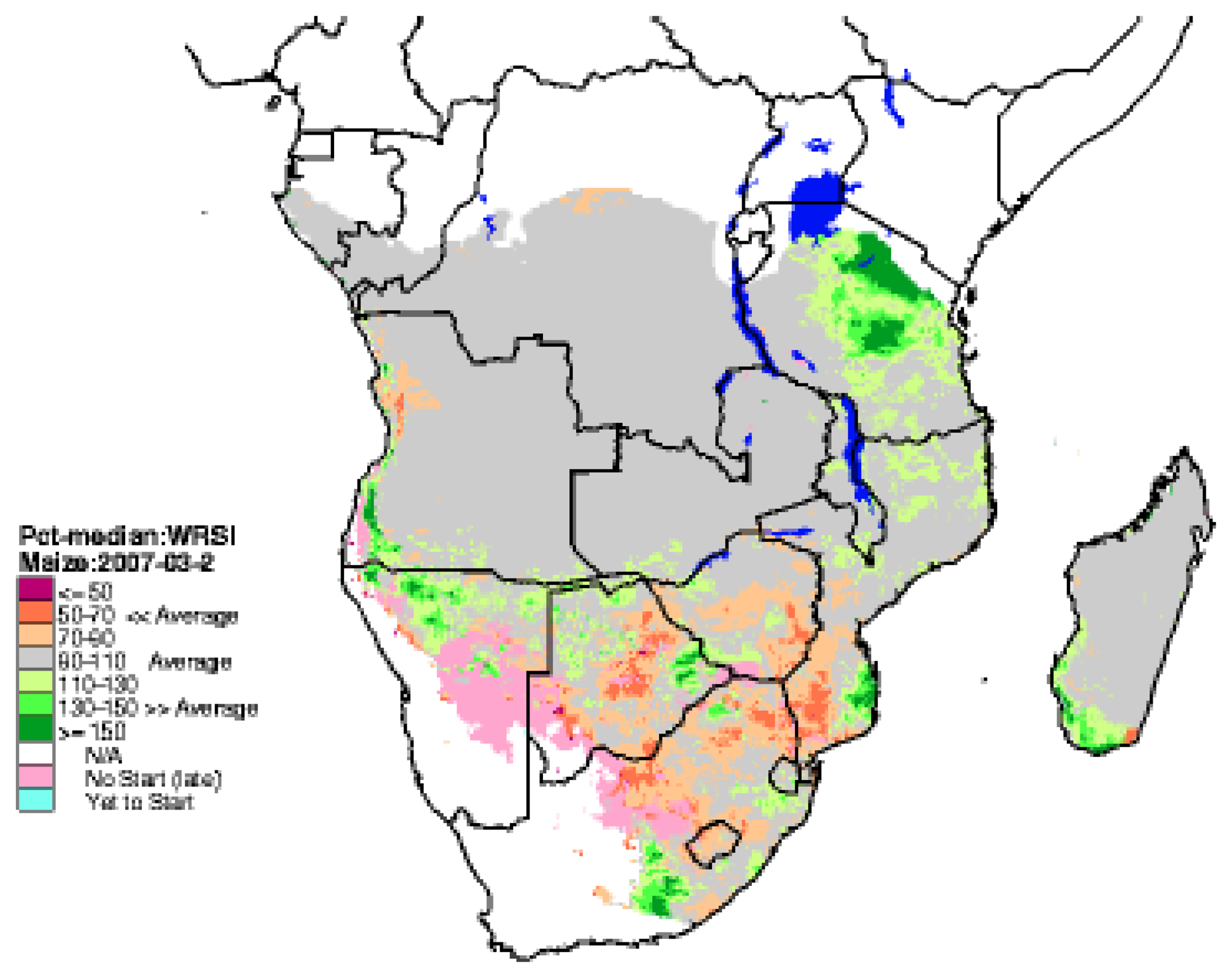
Figure 13 shows the WRSI anomaly as of the 2nd dekad of March, 2007 for the same southern Africa region. This is another way of looking at the model output to cancel out some of the potential wrong model assumptions such as the assumed length of the growing season. The WRSI anomaly is generated by calculating the extended WRSI (Figure 13) as a percentage of the median WRSI generated using median rainfall distribution. Figure 13 shows that much of southern Africa has performed about “average” (90 – 110%) compared to the median WRSI. On the other hand, a large part of southern Africa, southern Mozambique, Botswana and southern Zimbabwe have performed below average (70-90%) or much below average (50-70%). On the other hand isolated regions such are north central Tanzania have performed above average (> 130%). This relative description is corroborated by field reports in that there was a wide-spread yield reduction in much of the southern regions and an improved crop performance in Tanzania.
5. Future directions of remote sensing
The advances made in spaceborne remote sensing in the last 50 years, from sputnik 1 to Worldview-1, has been phenomenal. The present trends point to increasing several innovations. First, availability of data from multiple sensors with wide array of spatial, spectral, and radiometric characteristics. These data will be available from multiple sources. Second, significant advances have been made in harmonizing and synthesizing data from multiple sources that facilitates the use of data from these sensors of widely differing characteristics and sources. We also expect vendors to market data from multiple sources by harmonizing and by adding value. Third, availability of data from a constellation such as from Rapideye at very high resolution of 6.5 meter, in five bands including a red-edge band, and with ability to cover the entire world in 13-day frequency is a likely attractive form of data collection. This will certainly require innovations in data handling, storage, and backup. But for applications, a combination of very high spatial resolution and frequent coverage is very attractive. Fourth, the micro satellites that specialize in gathering data for specific geographic location and\or for particular applications are likely to become more attractive. Fifth, for many environmental and natural resource applications global wall-to-wall coverage is essential and here satellites like Landsat will continue to play most important role. Sixth, data availability in hyperspectral and hyperspatial sensors brings in new challenges in data mining, processing, backup, and retrieval. Seventh, the advances made in data synthesis, presentation, and accessibility through systems such as Google Earth will bring in new users and multiply applications of remote sensing in environmental sciences and natural resources management.
The authors expect that the future needs of the spatial data will be met overwhelmingly by spaceborne remote sensing.
References
- Adams, J.B.; Smith, M.O.; Johnson, P.E. Spectral mixture modeling: A new analysis of roack and soil types at the Viking Lander site. Journal of Geophysical Research 1986, 91, 8098–8112. [Google Scholar]
- Adams, J.B.; Sabol, D.E.; Kapos, V.; Filho, R.A.; Roberts, D.A.; Smith, M.O.; Gillespie, A.R. Classification of multispectral images based on fractions of endmembers: application to land cover change in the Brazilian Amazon. Remote Sensing of Environment 1995, 52, 137–154. [Google Scholar]
- Agbu, P.A.; James, M.E. NOAA/NASA Pathfinder AVHRR Land Data Set User's Manual; Greenbelt; Goddard Distributed Active Archive Center, NASA Goddard Space Flight Center, 1994. [Google Scholar]
- Allen, R.G.; Pereira, L.; Raes, D.; Smith, M. 1998; Crop Evapotranspiration; Food and Agriculture Organization of the United Nations: Rome, Italy, FAO publication 56; p. 290, ISBN 92-5-104219-5. [Google Scholar]
- Allen, R.G.; Tasurmi, M.; Morse, A.T.; Trezza, R. A Landsat-based Energy Balance and Evapotranspiration Model in Western US Water Rights Regulation and Planning. Journal of Irrigation and Drainage Systems 2005, 19(3-4), 251–268, 18. [Google Scholar]
- Aguiar, A.P.D.; Shimabukuro, Y.E.; Mascarenhas, N.D.A. Use of synthetic bands derived from mixing models in the multispectral classification of remote sensing images. International Journal of Remote Sensing 1999, 20, 647–657. [Google Scholar]
- Anderson, J.R.; Hardy, E.E.; Roach, T.J.; Whitmer, R.E. A Land Use and Land Cover Classification System for Use with Remote Sensor Data.; U.S. Geol. Survey Prof. Pap. 964; U.S. Gov. Print. Office: Washington DC, 1976. [Google Scholar]
- Arnold, C.L., Jr.; Gibbons, C.J. Impervious surface coverage: the emergence of a key environmental indicator. Journal of the American Planning Association 1996, 62, 243–258. [Google Scholar]
- Asner, G.P.; Lobell, D.B. A biogeophysical approach for automated SWIR unmixing of soils and vegetation. Remote Sensing of Environment 2000, 74, 99–112. [Google Scholar]
- Avery; Berlin. Fundamentals of Remote Sensing and Airphoto Interpretation, 5th Ed. ed; Macmillan Publishing Company: New York, 1992; p. 472. [Google Scholar]
- Bailey, G.B.; Lauer, D.T.; Carneggie, D.M. International collaboration: the cornerstone of satellite land remote sensing in the 21st century. Space Policy 2001, 17(3), 161–169. [Google Scholar]
- Bastiaanssen, W.G.M.; Menenti, M.; Feddes, R.A.; Holtslag, A.A.M. A remote sensing surface energy balance algorithm for land (SEBAL): 1) Formulation. Journal of Hydrology 1998, 212(213), 213–229. [Google Scholar]
- Boardman, J.W. Automated spectral unmixing of AVIRIS data using convex geometry concepts. In Summaries of the Fourth JPL Airborne Geoscience Workshop; JPL Publication 93-26; NASA Jet Propulsion Laboratory: Pasadena, Calif., 1993; pp. 11–14. [Google Scholar]
- Boardman, J.M.; Kruse, F.A.; Green, R.O. Mapping target signature via partial unmixing of AVIRIS data. In Summaries of the Fifth JPL Airborne Earth Science Workshop; JPL Publication 95–1; NASA Jet Propulsion Laboratory: Pasadena, Calif., 1995; pp. 23–26. [Google Scholar]
- Carlson, T.N.; Arthur, S.T. The impact of land use-land cover Changes due to urbanization on surface microclimate and hydrology: a Satellite Perspective. Global and Planetary Change 2000, 25, 49–65. [Google Scholar]
- Carlson, T.N.; Ripley, A.J. On the relationship between fractional vegetation cover, leaf area index and NDVI. Remote Sensing in Environment 1997, 62, 241–252. [Google Scholar]
- Che, N.; Price, J.C. Survey of radiometric calibration results and methods for visible and near-infrared channels of NOAA-7,-9 and −11 AVHRRs. Remote Sensing in Environment 1992, 41, 19–27. [Google Scholar]
- Cochrane, M.A.; Souza, C.M., Jr. Linear mixture model classification of burned forests in the eastern Amazon. International Journal of Remote Sensing 1998, 19, 3433–3440. [Google Scholar]
- Manual of Remote Sensing, 2nd Ed.; Colwell, R.N. (Ed.) American Society for Photogrammetry and Remote Sensing: Falls Church, Virginia, 1983.
- Devine, R. The Sputnik Challenge; Oxford University Press: New York: NY, 1993. [Google Scholar]
- Eye in the Sky: The Story of the Corona Spy Satellites; Dwayne, A.D.; Logsdon, J.M.; Latell, B. (Eds.) Smithsonian Books: Washington, DC, 1988; ISBN: 1560988304 (ISBN 1-56098-773-1 (paperback) or ISBN 1-56098-830-4 (hardcover)).
- Doorenbos, J.; Pruitt, W.O. Crop water requirements; Food and Agricultural Organization of the United Nations; FAO Irrigation and Drainage Paper 24; Rome, Italy, 1977. [Google Scholar]
- Earth Resources Data Analysis System (ERDAS) (1999) ERDAS Field guide; ERDAS Inc: Atlanta, GA.
- FAO. FAO/UNESCO soil map of the World: revised legend.; Food and Agricultural Organization of the United Nations; FAO World Resources Report 60; Rome, Italy, 1988. [Google Scholar]
- Florinsky, I.V. Relationships between topographically expressed zones of flow accumulation and sites of fault intersection: Analysis by means of digital terrain modeling. Environmental Modeling and Software 2000, 15, 87–100. [Google Scholar]
- House, F.B.; Gruber, A.; Hunt, G.E.; Mecherikunnel, A.T. History of satellites missions and measurements of the Earth Radiation Budget (1957-1984) Reviews of geophysics. 1986, 24, 357–377, ISSN 8755-1209.
- Jensen, J.R. Remote Sensing of the Environment: An Earth Resource Perspective, 2nd Ed. ed; Prentice-Hall, Inc.: Upper Saddle River, NJ, 2000; p. 544. [Google Scholar]
- Kramer, H.J. Observation of the Earth and its Environment: Survey of Missions and Sensors, 4th Ed. ed; Springer Verlag: Berlin, 2002; ISBN 3-540-42388-5.322. [Google Scholar]
- Kulagina, T.B.; Meshalkina, J.L.; Florinsky, I.V. The effect of topography on the distribution of landscape radiation temperature. Earth Observation and Remote Sensing 1995, 12, 448–458. [Google Scholar]
- Lee, S.; Lathrop, R.G., Jr. Sub-pixel estimation of urban land cover components with linear mixture model analysis and Landsat Thematic Mapper imagery. International Journal of Remote Sensing 2005, 26(22), 4885–4905. [Google Scholar]
- Lu, D.; Weng, Q. Spectral mixture analysis of the urban landscapes in Indianapolis with Landsat ETM+ imagery. Photogrammetric Engineering and Remote Sensing 2004, 70, 1053–1062. [Google Scholar]Lu, D.; Weng, Q. Use of impervious surface in urban land use classification. Remote Sensing of Environment 2006, 102(1-2), 146–160. [Google Scholar]Lu, D.; Weng, Q. Spectral mixture analysis of ASTER imagery for examining the relationship between thermal features and biophysical descriptors in Indianapolis, Indiana. Remote Sensing of Environment 2006, 104(2), 157–167. [Google Scholar]
- Madhavan, B.B.; Kubo, S.; Kurisaki, N.T.; Sivakumar, V.L.N. Appraising the anatomy and spatial growth of the Bangkok Metropolitan area using a vegetation-impervious-soil model through remote sensing. International Journal of Remote Sensing 2001, 22, 789–806. [Google Scholar]
- Mather, P.M. Land cover classification revisited. In Advances in Remote Sensing and GIS; Atkinson, P.M., Tate, N.J., Eds.; John Wiley & Sons: New York, 1999; pp. 7–16. [Google Scholar]
- McGwire, K.; Minor, T.; Fenstermaker, L. Hyperspectral mixture modeling for quantifying sparse vegetation cover in arid environments. Remote Sensing of Environment 2000, 72, 360–374. [Google Scholar]
- Melesse, A.M.; Nangia, V.; Wang, X. Hydrology and Water Balance of Devils Lake Basin: Part 1. Hydrometeorological Analysis and Lake Surface Area Mapping. J. of Spatial Hydrology 2006, 6(1), 120–132. [Google Scholar]
- Melesse, A.M.; Nangia, V.; Wang, X. Hydrology and Water Balance of Devils Lake Basin: Part 2. Grid-Based Spatial Surface Water Balance Modeling. J. of Spatial Hydrology 2006, 6(1), 133–144. [Google Scholar]
- Melesse, A.M. DEM-RS-GIS based storm runoff response study of Heart River sub-basin, Missouri River Basin. J. of Environmental Hydrology 2004, 12, 4. [Google Scholar]
- Melesse, A.M.; Jordan, J.D. Spatially Distributed Watershed Mapping and Modeling: Land Cover and Microclimate Mapping using Landsat Imagery Part 1. J. of Spatial Hydrology 2003, 3, 2. [Google Scholar]Melesse, A.M.; Graham, W. Spatially Distributed Watershed Mapping and Modeling: GIS-Based Storm Runoff Response and Hydrograph Analysis Part 2. J. of Spatial Hydrology 2003, 3, 2. [Google Scholar]
- Melesse, A.M. Spatiotemporal Dynamics of land surface parameters in the Red River of the North Basin. Physics and Chemistry of Earth 2004, 29, Special Issue: Anthropogenic impacts on catchment processes. 795–810. [Google Scholar]
- Melesse, A.; Wang, X. Impervious Surface Area Dynamics and Storm Runoff Response. In Remote Sensing of Impervious Surfaces; CRC Press/Taylor & Francis, 2007; Volume 19, pp. 369–384. [Google Scholar]
- Melesse, A.M.; Nangia, V. Spatially distributed surface energy flux estimation using remotely-sensed data from agricultural fields. Hydrological Processes 2005, 19(14), 2653–2670. [Google Scholar]
- Meyer, S.J.; Hubbard, K.G.; Wilhite, D. A crop specific drought index for corn: I. Model Development and Validation. Agronomy Journal 1993, 86, 388–395. [Google Scholar]
- Oberg, J.; Melesse, A. Evapotranspiration Dynamics at an Ecohydrological Restoration Site: An Energy Balance and Remote Sensing Approach. J. of American Water Resources Association 2006, 42(3), 565–582. [Google Scholar]
- Oke, T.R. The energetic basis of the urban heat island. Quarterly Journal of the Royal Meteorological Society 1982, 108, 1–24. [Google Scholar]
- Owen, T.W.; Carlson, T.N.; Gillies, R.R. Remotely-sensed Surface Parameters Governing Urban Climate Change. Int. J. of Remote Sensing 1998, 19, 1663–1681. [Google Scholar]
- Phinn, S.; Stanford, M.; Scarth, P.; Murray, A.T.; Shyy, P.T. Monitoring the composition of urban environments based on the vegetation-impervious surface-soil (VIS) model by subpixel analysis techniques. International Journal of Remote Sensing 2002, 23, 4131–4153. [Google Scholar]
- Powell, R.L.; Roberts, D.A.; Dennison, P. E.; Hess, L.L. Sub-pixel mapping of urban land cover using multiple end-member spectral mixture analysis: Manaus, Brazil. Remote Sensing of Environment 2007, 106(2), 253–267. [Google Scholar]
- Price, J.C. Calibration of satellite radiometers and the comparison of vegetation indices. Remote Sensing of Environment 1987, 21, 15–27. [Google Scholar]
- Rashed, T.; Weeks, J.R.; Roberts, D.A.; Rogan, J.; Powell, R. Measuring the physical composition of urban morphology using multiple end-member spectral mixture models. Photogrammetric Engineering and Remote Sensing 2003, 69, 1011–1020. [Google Scholar]
- Rashed, T.; Weeks, J.R.; Stow, D.; Fugate, D. Measuring temporal compositions of urban morphology through spectral mixture analysis: toward a soft approach to change analysis in crowded cities. International Journal of Remote Sensing 2005, 26(4), 699–718. [Google Scholar]
- Ridd, M.K. Exploring a V-I-S (Vegetation-Impervious Surface-Soil) model for urban ecosystem analysis through remote sensing: comparative anatomy for cities. International Journal of Remote Sensing 1995, 16, 2165–2185. [Google Scholar]
- Senay, G.B.; Verdin, J. Characterization of yield reduction in Ethiopia using a GIS-based crop water balance model. Canadian Journal of Remote Sensing 2003, 29(6), 687–692. [Google Scholar]
- Senay, G.B.; Budde, M.; Verdin, J.P.; Melesse, A.M. A coupled remote sensing and simplified surface energy balance approach to estimate actual evapotranspiration from irrigated fields. Sensors 2007, 7, 979–1000. [Google Scholar]
- Senay, G.B.; Verdin, J.P.; Lietzow, R.; Melesse, A.M. Global daily reference vapotranspiration modeling and validation. Journal of American Water Resources Research 2007. In press. [Google Scholar]
- Setiawan, H.; Mathieu, R.; Thompson-Fawcet, M. Assessing the applicability of the V-I-S model to map urban land use in the developing world: Case study of Yogyakarta, Indonesia. Computers, Environment and Urban Systems 2006, 30(4), 503–522. [Google Scholar]
- Small, C. Estimation of urban vegetation abundance by spectral mixture analysis. International Journal of Remote Sensing 2001, 22, 1305–1334. [Google Scholar]
- Smith, M. Expert consultation on revision of FAO methodologies for crop water requirements; Food and Agricultural Organization of the United Nations; FAO Publication 73; Rome, Italy, 1992. [Google Scholar]
- Stoney, W. A Guide to the Global Explosion of Land-Imaging Satellites; Markets and Opportunities. 2005. http://www.eijournal.com/.http://www.geog.ucsb.edu/∼jeff/115a/remotesensinghistory.html.
- Thenkabail, P.S.; Biradar, C.M.; Turral, H.; Noojipady, P.; Li, Y.J.; Vithanage, J.; Dheeravath, V.; Velpuri, M.; Schull, M.; Cai, X.L.; Dutta, R. An Irrigated Area Map of the World (1999) derived from Remote Sensing. Research Report # 105; International Water Management Institute, 2006; p. 74. Also, see under documents in: http://www.iwmigiam.org.
- Thenkabail, P.S.; Enclona, E.A.; Ashton, M.S.; Legg, C.; Jean De Dieu, M. Hyperion, IKONOS, ALI, and ETM+ sensors in the study of African rainforests. Remote Sensing of Environment 2004, 90, 23–43. [Google Scholar]
- Thenkabail, P.S. Inter-sensor relationships between IKONOS and Landsat-7 ETM+ NDVI data in three ecoregions of Africa. Int. J. Remote Sensing 2004, 25(2), 389–408. [Google Scholar]
- Tucker, C.J.; Grant, D.M.; Dykstra, J.D. NASA's Global Orthorectified Landsat Dataset. Photogrammetric Engineering & Remote Sensing 2005, 70(3), 313. [Google Scholar]
- Verdin, J.; Klaver, R. Grid cell based crop water accounting for the famine early warning system. Hydrological Processes 2002, 16, 1617–1630. [Google Scholar]
- Wang, F. Fuzzy supervised classification of remote sensing images. IEEE Transactions on Geoscience and Remote Sensing 1990, 28(2), 194–201. [Google Scholar]
- Ward, D.; Phinn, S. R.; Murray, A.T. Monitoring growth in rapidly urbanizing areas using remotely sensed data. The Professional Geographer 2000, 53, 371–386. [Google Scholar]
- Weng, Q.; Lu, D.; Schubring, J. Estimation of land surface temperature-vegetation abundance relationship for urban heat island studies. Remote Sensing of Environment 2004, 89, 467–483. [Google Scholar]
- Weng, Q.; Quattrochi, D.A. Urban Remote Sensing; CRC Press/Taylor and Francis, 2006; p. p. 448. [Google Scholar]
- Weng, Q. Remote Sensing of Impervious Surfaces; CRC Press/Taylor and Francis, 2007; p. p. 454. [Google Scholar]
- Wu, C.; Murray, A.T. Estimating impervious surface distribution by spectral mixture analysis. Remote Sensing of Environment 2003, 84, 93–505. [Google Scholar]
- Wu, J.G.; Jelinski, D.E.; Luck, M.; Tueller, P.T. Multiscale analysis of landscape heterogeneity: Scale variance and pattern metrics. Geographic Information Sciences 2000, 6(1), 6–19. [Google Scholar]
- Wu, J.W.; Xu, J.H.; Yue, W.Z. V-I-S model for cities that are experiencing rapid urbanization and development. Geoscience and Remote Sensing Symposium, IGARSS'05. Proceedings; 2005; 3, pp. 1503–1506. [Google Scholar]
- Xie, P.; Arkin, P.A. Global Precipitation: A 17-year monthly analysis based on gauge observations, satellite estimates and numerical model outputs. Bulletin of the American Meteorological Society 1997, 78(11), 2539–2558. [Google Scholar]
Acronyms and Abbreviations
| ASTER | Advanced Space borne Thermal Emission and Reflection Radiometer |
| ALI | Advanced Land Imager |
| AVHRR | Advanced Very High Resolution Radiometer |
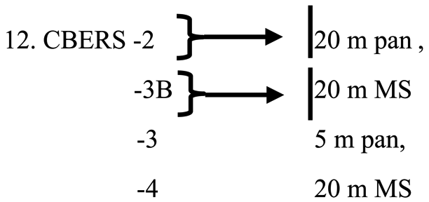
| CBERS -2 | China-Brazil Earth Resources Satellite |
| FORMOSAT | Taiwanis Satellite Operated by Taiwanis National Space Organization NSPO. Data Marketed by SPOT |
| Hyperion | First Spaceborne Hyperspectral Sensor Onboard Earth Observing-1(EO-1) |
| IKONOS | High-Resolution Satellite Operated by GeoEye |
| IRS-1C/D-LISS | Indian Remote Sensing Satellite /Linear Imaging Self Scanner |
| IRS-P6-AWiFS | Indian Remote Sensing Satellite/Advanced Wide Field Sensor |
| KOMFOSAT | Korean Multipurpose Satellite. Data Marketed by SPOT Image |
| Landsat-1, 2, 3 MSS | Multi Spectral Scanner |
| Landsat-4, 5 TM | Thematic Mapper |
| Landsat-7 ETM+ | Enhanced Thematic Mapper Plus |
| MODIS | Moderate Imaging Spectral Radio Meter |
| QUICKBIRD | Satellite from DigitalGlobe, a private company in USA |
| RAPID EYE – A/E | Satellite constellation from Rapideye, a German company |
| RESOURSESAT | Satellite launched by the India |
| SPOT | Satellites Pour l'Observation de la Terre or Earth-observing Satellites |
| SWIR | Short Wave Infrared Sensor |
| VNIR | Visible Near-Infrared Sensor |
| WORLDVIEW |
Figure 1.
Land-use/land-cover map of Indianapolis, United States, derived from a Landsat ETM+ image of June 22, 2000.
Figure 1.
Land-use/land-cover map of Indianapolis, United States, derived from a Landsat ETM+ image of June 22, 2000.
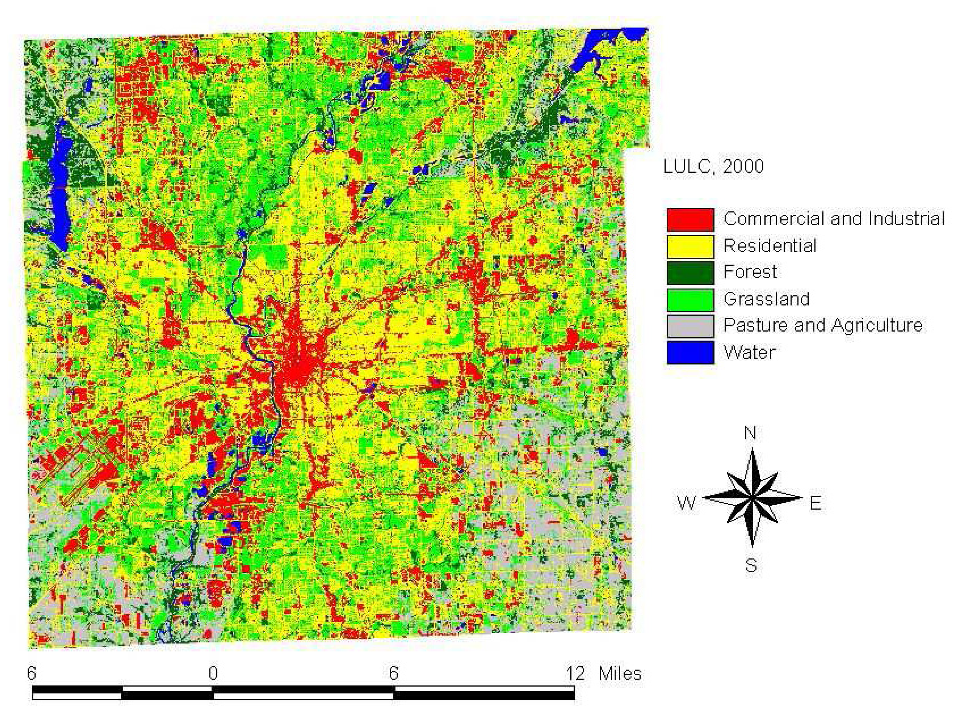
Figure 2.
Impervious surface images of Indianapolis derived from a Terra's ASTER image of June 16, 2001.
Figure 2.
Impervious surface images of Indianapolis derived from a Terra's ASTER image of June 16, 2001.
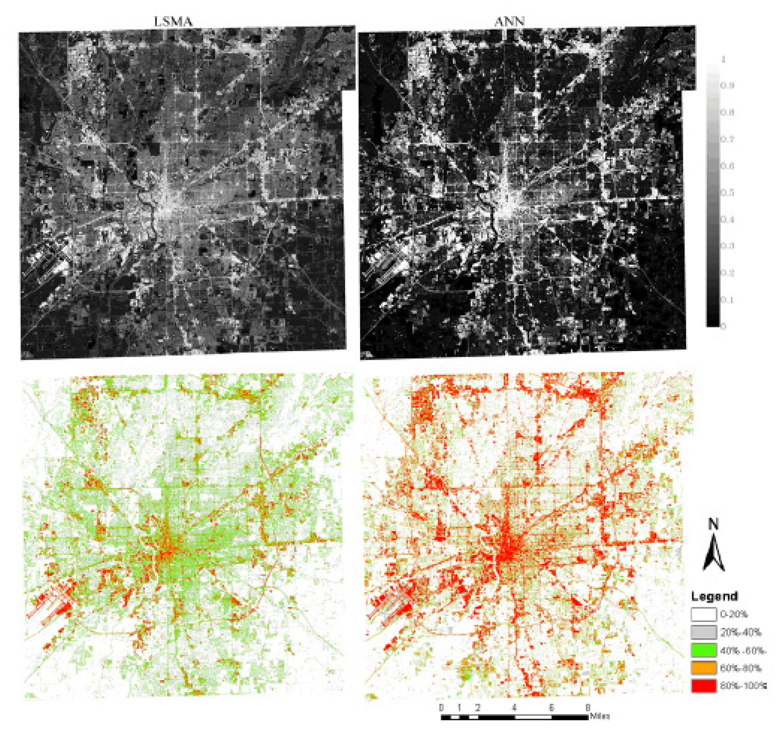
Figure 3.
The spatial expansion of Devils Lake from Landsat images.
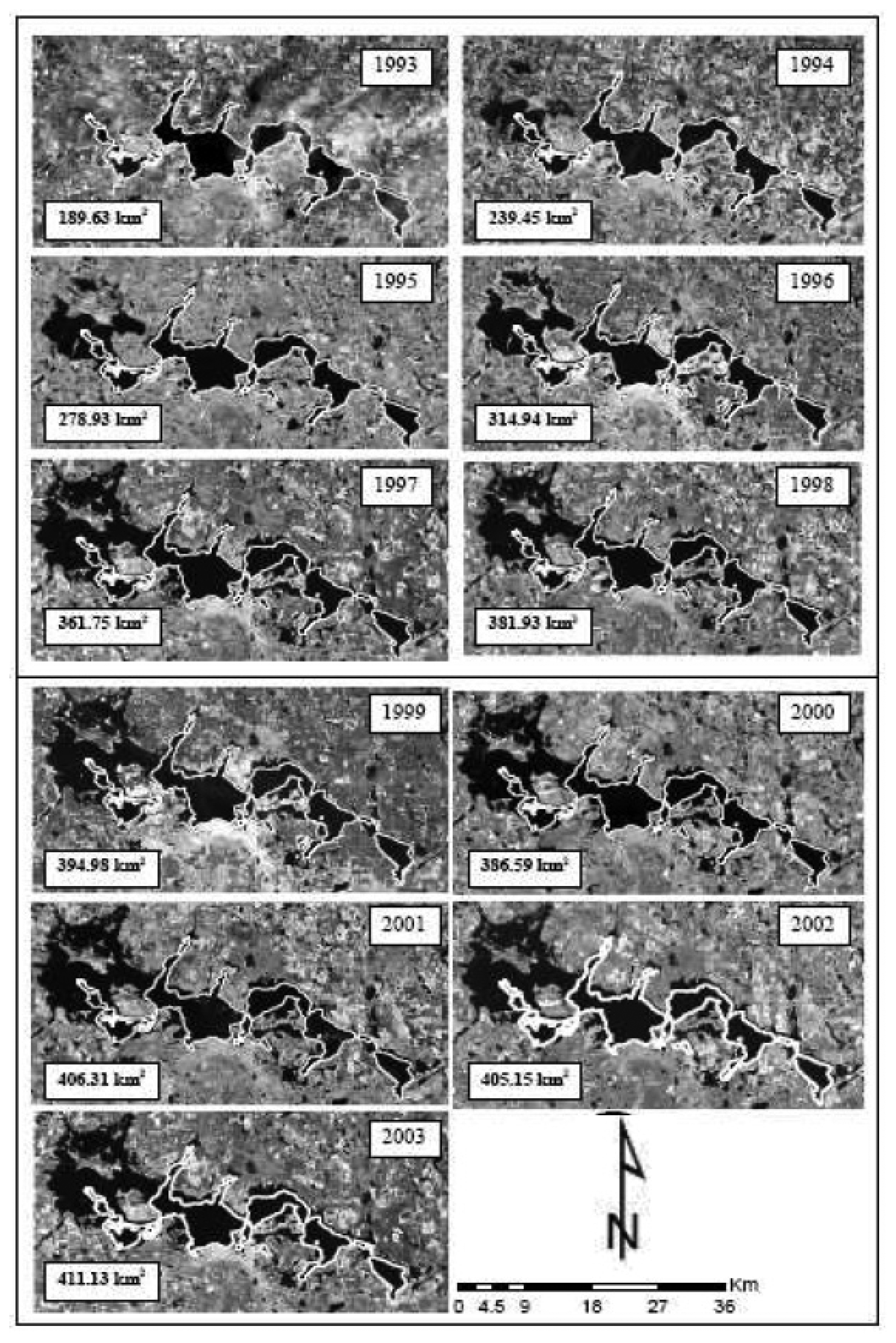
Figure 4.
Devils Lake surface area progressions from Landsat images.

Figure 5.
Land cover mapping: (a) Scattergram of NDVI vs surface temperature (b) Land cover classes of Heart River sub-basin, Missouri River basin.
Figure 5.
Land cover mapping: (a) Scattergram of NDVI vs surface temperature (b) Land cover classes of Heart River sub-basin, Missouri River basin.
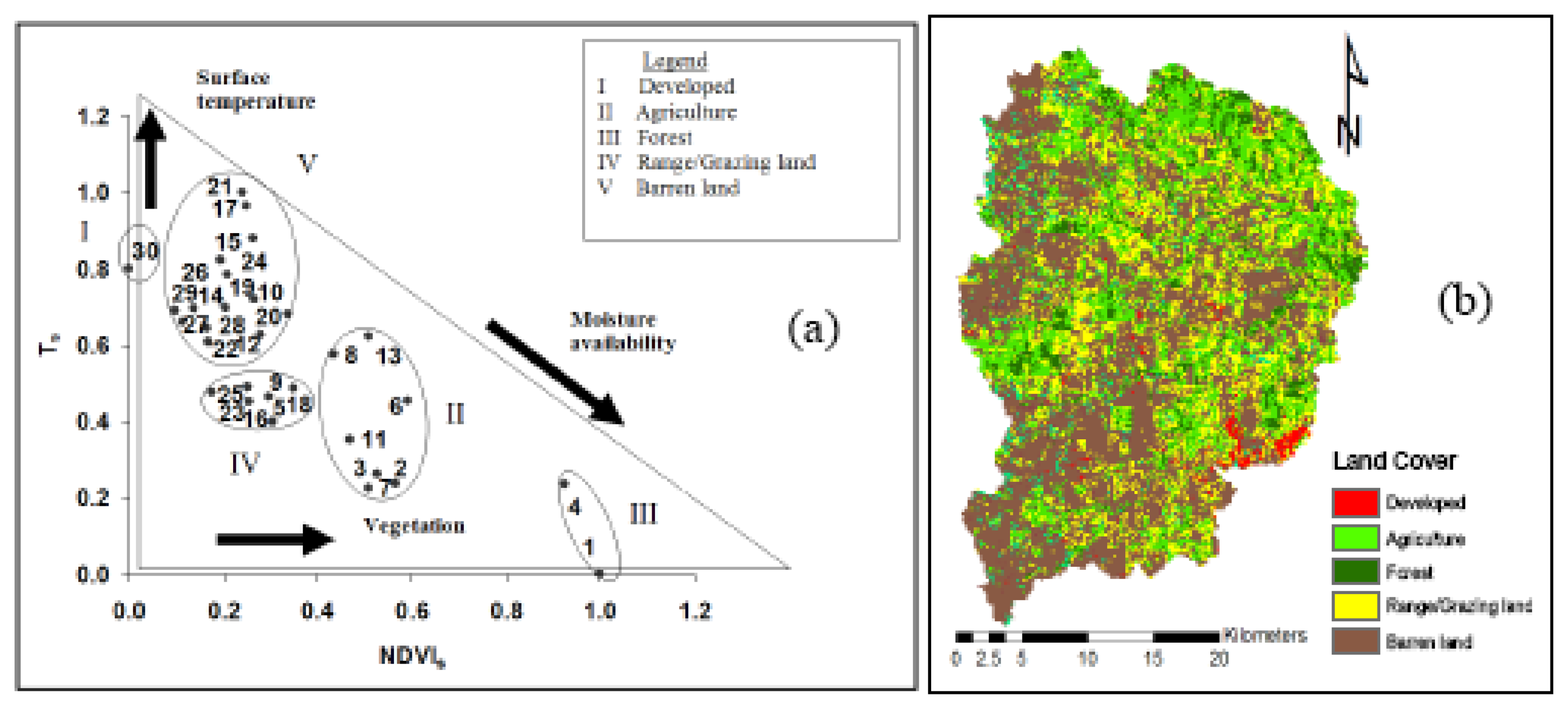
Figure 6.
Percent vegetation cover for Econlockhatchee River sub-basin (Econ sub-basin) in Florida (a) 1984 (b) 2000.
Figure 6.
Percent vegetation cover for Econlockhatchee River sub-basin (Econ sub-basin) in Florida (a) 1984 (b) 2000.
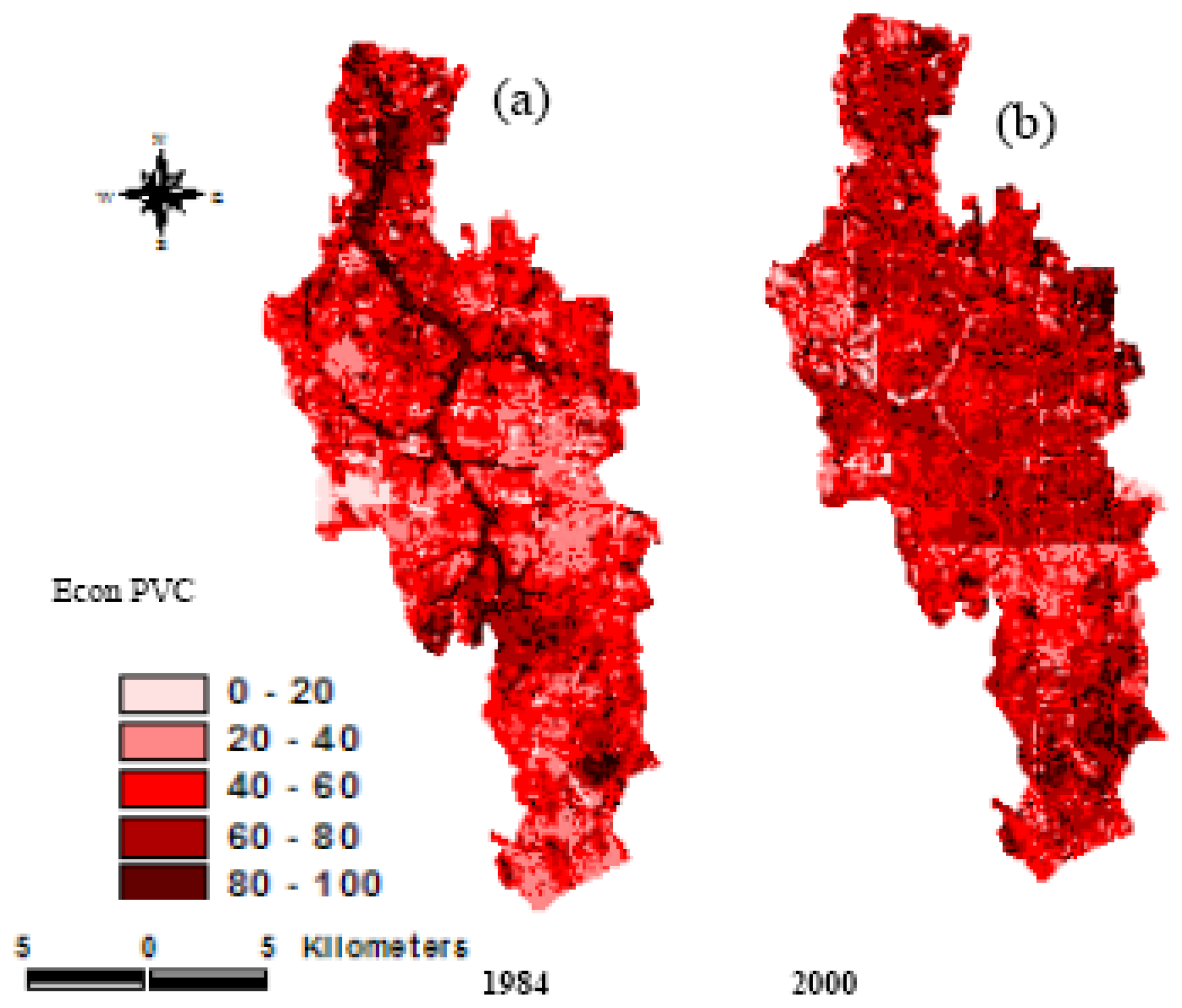
Figure 7.
Percent impervious surface area of South Florida from MODIS data.

Figure 8.
Wetness index of a wheat field in North Dakota as mapped from microtopography data.
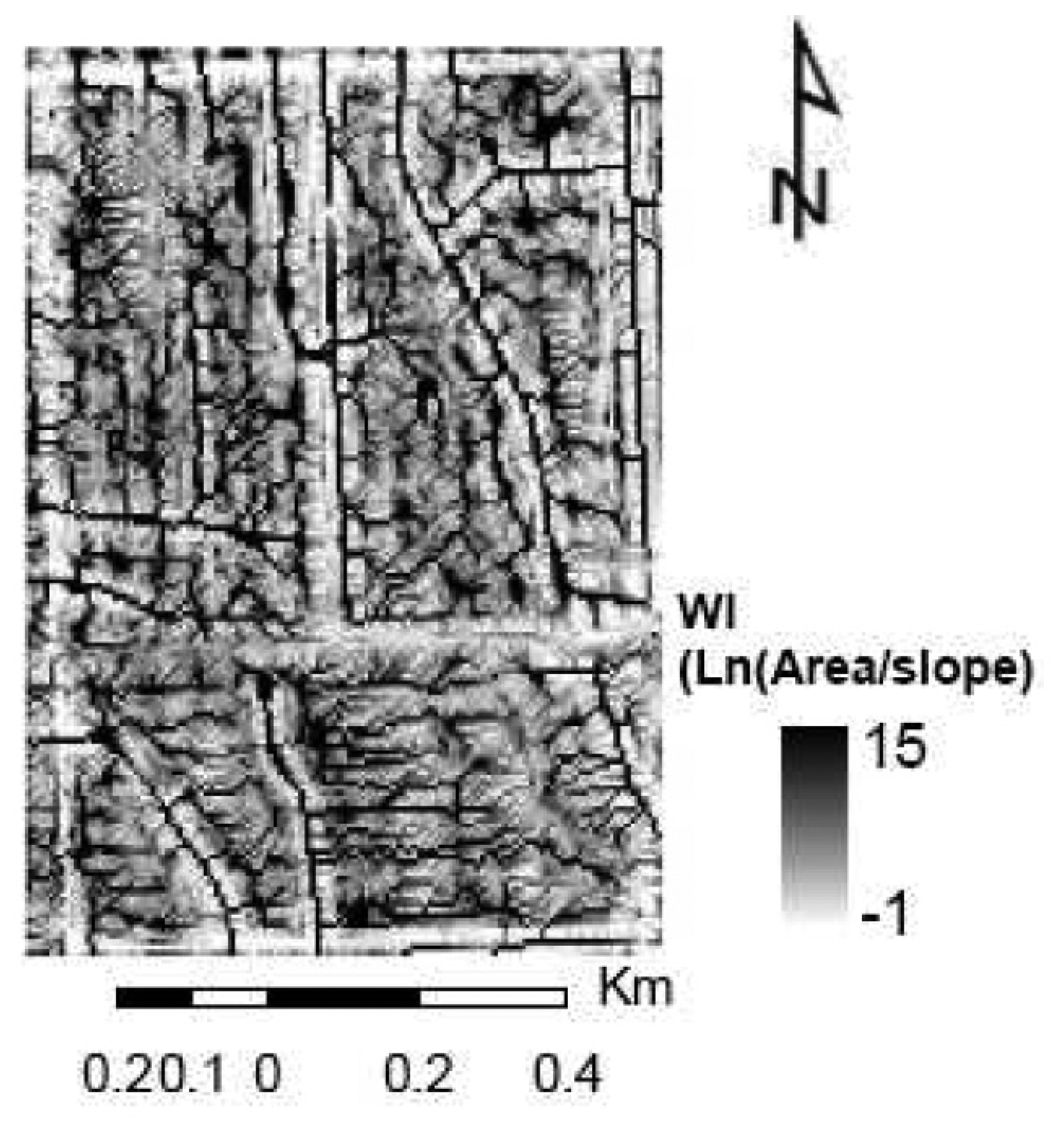
Figure 9.
Wetness index vs. latent heat flux for a wheat field.

Figure 10.
Onset of rains map for southern Africa for the 2006/2007 growing seasons as of the 2nd dekad of March, 2007.
Figure 10.
Onset of rains map for southern Africa for the 2006/2007 growing seasons as of the 2nd dekad of March, 2007.

Figure 11.
map of soil water index (SWI) which shows the level of soil water in the root zone as defined by the soil water holding capacity (WHC) of the top 1 m of soil.
Figure 11.
map of soil water index (SWI) which shows the level of soil water in the root zone as defined by the soil water holding capacity (WHC) of the top 1 m of soil.
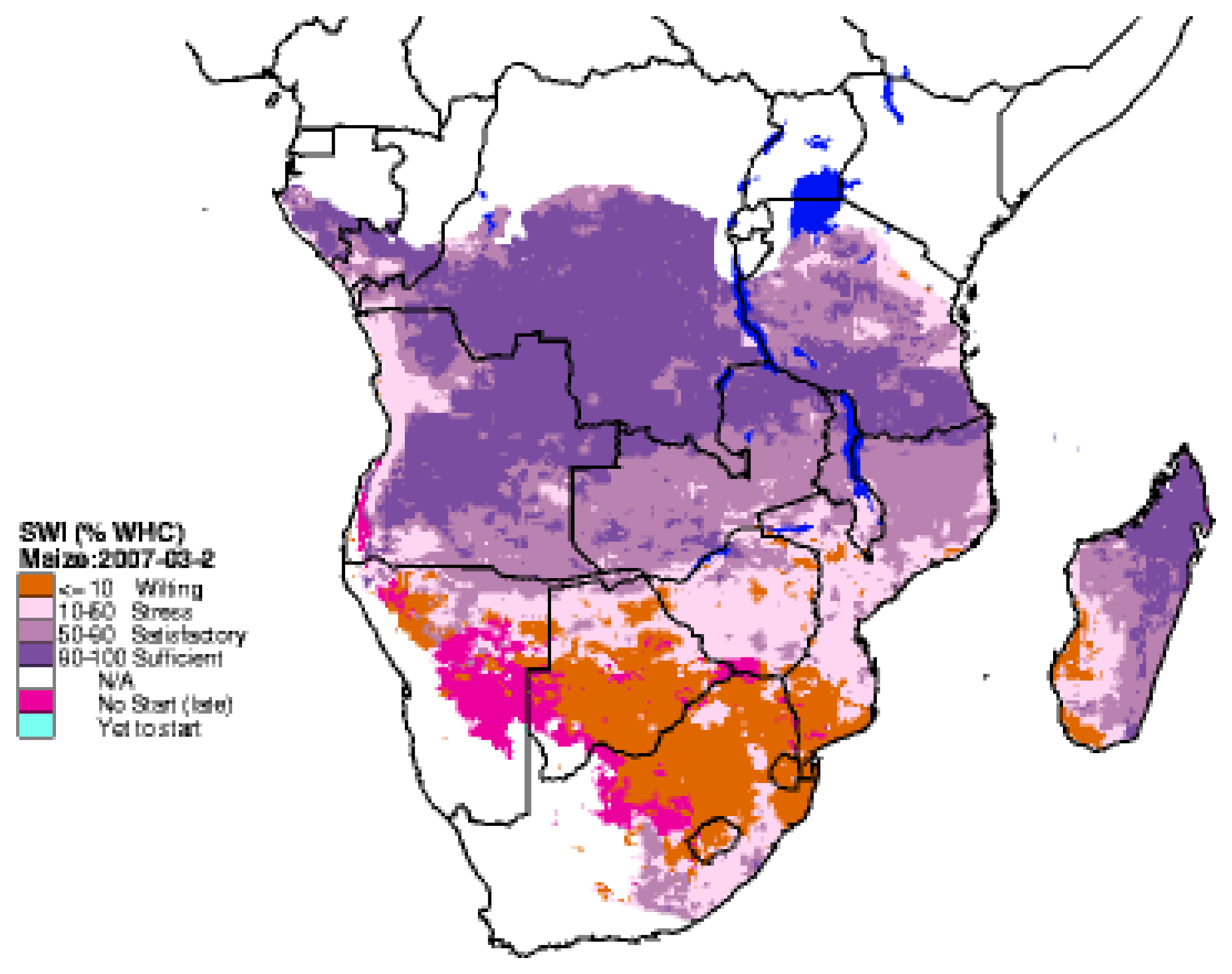
Figure 12.
Spatial distribution of maize crop water requirement satisfaction index (WRSI) for southern Africa as of the 2nd dekad of March 2007.
Figure 12.
Spatial distribution of maize crop water requirement satisfaction index (WRSI) for southern Africa as of the 2nd dekad of March 2007.
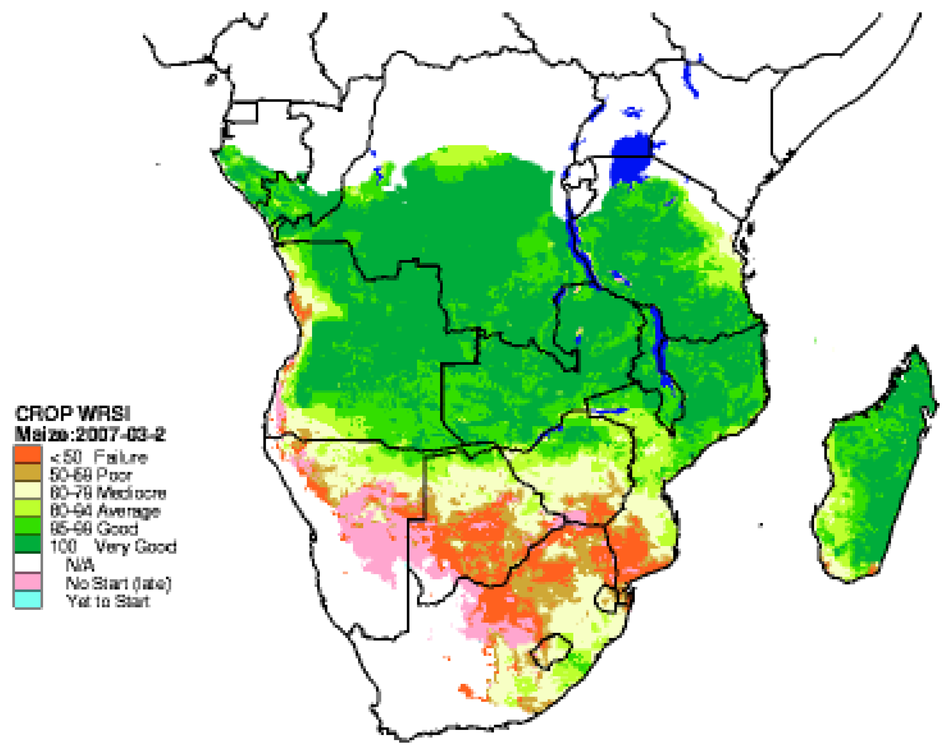
Figure 13.
WRSI anomaly as of the 2nd dekad of March, 2007 for the same southern Africa region.

| Sensor | Spatial (meters) | Spectral (#) | Radiometric (bit) | band range (μm) | band widths (μm) | Irradiance (W m2-sr-1 μm-1) | Data Points (# per hectares) | Frequency of revisit (days) | |||||||||||||||
|---|---|---|---|---|---|---|---|---|---|---|---|---|---|---|---|---|---|---|---|---|---|---|---|
| A.Coarse Resolution Sensors | |||||||||||||||||||||||
| 1. AVHRR | 1000 | 4 | 11 | 0.58-0.68 | 0.10 | 1390 | 0.01 | daily | |||||||||||||||
| 0.725-1.1 | 0.375 | 1410 | |||||||||||||||||||||
| 3.55-3.93 | 0.38 | 1510 | |||||||||||||||||||||
| 10.30-10.95 | 0.65 | 0 | |||||||||||||||||||||
| 10.95-11.65 | 0.7 | 0 | |||||||||||||||||||||
| 2. MODIS | 250, 500,1000 | 36/7 | 12 | 0.62-0.67 | 0.05 | 1528.2 | 0.16, 0.04, 0.01 | daily | |||||||||||||||
| 0.84-0.876 | 0.036 | 974.3 | 0.16, 0.04, 0.01 | ||||||||||||||||||||
| 0.459-0.479 | 0.02 | 2053 | |||||||||||||||||||||
| 0.545-0.565 | 0.02 | 1719.8 | |||||||||||||||||||||
| 1.23-1.25 | 0.02 | 447.4 | |||||||||||||||||||||
| 1.63-1.65 | 0.02 | 227.4 | |||||||||||||||||||||
| 2.11-2.16 | 0.05 | 86.7 | |||||||||||||||||||||
| B.Multi Spectral Sensors | |||||||||||||||||||||||
| 3. Landsat-1, 2, 3 | MSS 56X79 | 4 | 6 | 0.5-0.6 | 0.1 | 1970 | 2.26 | 16 | |||||||||||||||
| 0.6-0.7 | 0.1 | 1843 | |||||||||||||||||||||
| 0.7-0.8 | 0.1 | 1555 | |||||||||||||||||||||
| 0.8-1.1 | 0.3 | 1047 | |||||||||||||||||||||
| 4. Landsat-4, 5 TM | 30 | 7 | 8 | 0.45-0.52 | 0.07 | 1970 | 11.1 | 16 | |||||||||||||||
| 0.52-0.60 | 0.80 | 1843 | |||||||||||||||||||||
| 0.63-0.69 | 0.60 | 1555 | |||||||||||||||||||||
| 0.76-0.90 | 0.14 | 1047 | |||||||||||||||||||||
| 1.55-1.74 | 0.19 | 227.1 | |||||||||||||||||||||
| 10.4-12.5 | 2.10 | 0 | |||||||||||||||||||||
| 2.08-2.35 | 0.25 | 80.53 | |||||||||||||||||||||
| 5. Landsat-7 ETM+ | 30 | 8 | 8 | 0.45-0.52 | 0.65 | 1970 | 44.4, 11.1 | 16 | |||||||||||||||
| 0.52-0.60 | 0.80 | 1843 | |||||||||||||||||||||
| 0.63-0.69 | 0.60 | 1555 | |||||||||||||||||||||
| 0.50-0.75 | 0.150 | 1047 | |||||||||||||||||||||
| 0.75-0.90 | 0.200 | 227.1 | |||||||||||||||||||||
| 10.0 - 12.5 | 2.5 | 0 | |||||||||||||||||||||
| 1.75-1.55 | 0.2 | 1368 | |||||||||||||||||||||
| 0.52-0.90 (p) | 0.38 | 1352.71 | |||||||||||||||||||||
| 6. ASTER | 15, 30, 90 | 15 | 8 | 0.52-0.63 | 0.11 | 1846.9 | 44.4, 11.1, 1.23 | 16 | |||||||||||||||
| 0.63-0.69 | 0.06 | 1546.0 | |||||||||||||||||||||
| 0.76-0.86 | 0.1 | 1117.6 | |||||||||||||||||||||
| 0.76-0.86 | 0.1 | 1117.6 | |||||||||||||||||||||
| 1.60-1.70 | 0.1 | 232.5 | |||||||||||||||||||||
| 2.145-2.185 | 0.04 | 80.32 | |||||||||||||||||||||
| 2.185-2.225 | 0.04 | 74.96 | |||||||||||||||||||||
| 2.235-2.285 | 0.05 | 69.20 | |||||||||||||||||||||
| 2.295-2.365 | 0.07 | 59.82 | |||||||||||||||||||||
| 2.360-2.430 | 0.07 | 57.32 | |||||||||||||||||||||
| 12 | 8.125-8.475 | 0.35 | 0 | ||||||||||||||||||||
| 8.475-8.825 | 0.35 | 0 | |||||||||||||||||||||
| 8.925-9.275 | 0.35 | 0 | |||||||||||||||||||||
| 10.25-10.95 | 0.7 | 0 | |||||||||||||||||||||
| 10.95-11.65 | 0.7 | 0 | |||||||||||||||||||||
| 7. ALI | 30 | 10 | 12 | .048-0.69 (p) | 0.64 | 1747.8600 | |||||||||||||||||
| 0.433-0.453 | 0.20 | 1849.5 | 11.1 | 16 | |||||||||||||||||||
| 0.450-0.515 | 0.65 | 1985.0714 | |||||||||||||||||||||
| 0.425-0.605 | 0.80 | 1732.1765 | |||||||||||||||||||||
| 0.633-0.690 | 0.57 | 1485.2308 | |||||||||||||||||||||
| 0.775-0.805 | 0.30 | 1134.2857 | |||||||||||||||||||||
| 0.845-0.890 | 0.45 | 948.36364 | |||||||||||||||||||||
| 1.200-1.300 | 1.00 | 439.61905 | |||||||||||||||||||||
| 1.550-1.750 | 2.00 | 223.39024 | |||||||||||||||||||||
| 2.080-2.350 | 2.70 | 78.072727 | |||||||||||||||||||||
| 8. SPOT-1 | 2. 5-20 | 15 | 16 | 0.50-0.59 | 0.09 | 1858 | 1600, 25 | 3-5 | |||||||||||||||
| -2 | 0.61-0.68 | 0.07 | 1575 | ||||||||||||||||||||
| -3 | 0.79-0.89 | 0.1 | 1047 | ||||||||||||||||||||
| -4 | 1.5-1.75 | 0.25 | 234 | ||||||||||||||||||||
| 0.51-0.73 (p) | 0.22 | 1773 | |||||||||||||||||||||
| 9. IRS-1C | 23.5 | 15 | 8 | 0.52-0.59 | 0.07 | 1851.1 | 18.1 | 16 | |||||||||||||||
| 0.62-0.68 | 0.06 | 1583.8 | |||||||||||||||||||||
| 0.77-0.86 | 0.09 | 1102.5 | |||||||||||||||||||||
| 1.55-1.70 | 0.15 | 240.4 | |||||||||||||||||||||
| 0.5-0.75 (P) | 0.25 | 1627.1 | |||||||||||||||||||||
| 10. IRS-1 | 23.5 | 15 | 8 | 0.52-0.59 | 0.07 | 1852.1 | 18.1 | 16 | |||||||||||||||
| 0.62-0.68 | 0.06 | 1577.38 | |||||||||||||||||||||
| 0.77-0.86 | 0.09 | 1096.7 | |||||||||||||||||||||
| 1.55-1.70 | 0.15 | 240.4 | |||||||||||||||||||||
| 0.5-0.75 (P) | 0.25 | 1603.9 | |||||||||||||||||||||
| 11. IRS-P6-AWiFS | 56 | 4 | 10 | 0.52-0.59 | 0.07 | 1857.7 | 3.19 | 16 | |||||||||||||||
| 0.62-0.68 | 0.06 | 1556.4 | |||||||||||||||||||||
| 0.77-0.86 | 0.09 | 1082.4 | |||||||||||||||||||||
| 1.55-1.70 | 0.15 | 239.84 | |||||||||||||||||||||
 | 20 m pan, | 11 | 0.51-0.73 | 0.22 | 1934.03 | 25, 25 | |||||||||||||||||
| 20 m MS | 0.45-0.52 | 0.07 | 1787.10 | ||||||||||||||||||||
| 5 m pan, | 0.52-0.59 | 0.07 | 1587.97 | 400, 25 | |||||||||||||||||||
| 20 m MS | 0.63-0.69 | 0.06 | 1069.21 | ||||||||||||||||||||
| 0.77-0.89 | 0.12 | 1664.3 | |||||||||||||||||||||
| C.Hyper-Spectral Sensor | |||||||||||||||||||||||
| 1. Hyperion | 30 | 196a | 16 | 196 effective | 10 nm wide | See data in | 11.1 | 16 | |||||||||||||||
| Calibrated bands | (approx.) for all | Neckel and Labs | |||||||||||||||||||||
| VNIR (band 8 to 57 | 196 bands | (1984). Plot it | |||||||||||||||||||||
| 427.55 to 925.85 nm | and obtain | ||||||||||||||||||||||
| SWIR (band 79 to 224) | values for | ||||||||||||||||||||||
| 932.72 to 2395.53 nm | Hyperion bands | ||||||||||||||||||||||
| D.Hyper-Spatial Sensor | |||||||||||||||||||||||
| 1. IKONOS | 1-4 | 4 | 11 | 0.445-0.516 | 0.71 | 1930.9 | 10000, 625 | 5 | |||||||||||||||
| 0.506-0.595 | 0.89 | 1854.8 | |||||||||||||||||||||
| 0.632-0.698 | 0.66 | 1156.5 | |||||||||||||||||||||
| 0.757-0.853 | 0.96 | 1156.9 | |||||||||||||||||||||
| 2. QUICKBIRD | 0.61-2.44 | 4 | 11 | 0.45-0.52 | 0.07 | 1381.79 | 14872, 625 | 5 | |||||||||||||||
| 0.52-0.60 | 0.08 | 1924.59 | |||||||||||||||||||||
| 0.63-0.69 | 0.06 | 1843.08 | |||||||||||||||||||||
| 0.76-0.89 | 0.13 | 1574.77 | |||||||||||||||||||||
| 3. RESOURSESAT | 5.8 | 3 | 10 | 0.52 - 0.59 | 0.07 | 1853.6 | 33.64 | 24 | |||||||||||||||
| 0.62 - 0.68 | 0.06 | 1581.6 | |||||||||||||||||||||
| 0.77 - 0.86 | 0.09 | 1114.3 | |||||||||||||||||||||
| 4. RAPID EYE - A | 6.5 | 5 | 12 | 0.44-0.51 | 0.07 | 1979.33 | 236.7 | 1-2 | |||||||||||||||
| - E | 0.52-0.59 | 0.07 | 1752.33 | ||||||||||||||||||||
| 0.63-0.68 | 0.05 | 1499.18 | |||||||||||||||||||||
| 0.69-0.73 | 0.04 | 1343.67 | |||||||||||||||||||||
| 0.77-0.89 | 0.12 | 1039.88 | |||||||||||||||||||||
| 5. WORLDVIEW | 0.55 | 1 | 11 | 0.45-0.51 | 0.06 | 1996.77 | 40000 | 1.7-5.9 | |||||||||||||||
| 6. FORMOSAT-2 | 2-8 | 5 | 11 | 0.45-0.52 | 0.07 | 1974.93 | 2500, 156.25 | daily | |||||||||||||||
| 0.52-0.60 | 0.08 | 1743.12 | |||||||||||||||||||||
| 0.63-0.69 | 0.06 | 1485.23 | |||||||||||||||||||||
| 0.76-0.90 | 0.14 | 1041.28 | |||||||||||||||||||||
| 0.45-0.90(p) | 0.45 | 1450 | |||||||||||||||||||||
| 7. KOMPSAT-2 | 1-4 | 5 | 10 | 0.5-0.9 | 0.4 | 1379.46 | 10000, 625 | 3-28 | |||||||||||||||
| 0.45-0.52 | 0.07 | 1974.93 | |||||||||||||||||||||
| 0.52-0.6 | 0.08 | 1743.12 | |||||||||||||||||||||
| 0.63-0.59 | 0.04 | 1485.23 | |||||||||||||||||||||
| 0.76-0.90 | 0.14 | 1041.28 | |||||||||||||||||||||
Note:
a= Of the 242 bands, 196 are unique and calibrated. These are: (A) Band 8 (427.55 nm) to band 57 (925.85 nm) that are acquired by visible and near-infrared (VNIR) sensor; and (B) Band 79 (932.72 nm) to band 224 (2395.53 nm) that are acquired by short wave infrared (SWIR) sensor
b= First band is panchromatic, rest Multi-Spectral
© 2007 by MDPI ( http://www.mdpi.org). Reproduction is permitted for noncommercial purposes.
Share and Cite
MDPI and ACS Style
Melesse, A.M.; Weng, Q.; Thenkabail, P.S.; Senay, G.B. Remote Sensing Sensors and Applications in Environmental Resources Mapping and Modelling. Sensors 2007, 7, 3209-3241. https://doi.org/10.3390/s7123209
AMA Style
Melesse AM, Weng Q, Thenkabail PS, Senay GB. Remote Sensing Sensors and Applications in Environmental Resources Mapping and Modelling. Sensors. 2007; 7(12):3209-3241. https://doi.org/10.3390/s7123209
Chicago/Turabian StyleMelesse, Assefa M., Qihao Weng, Prasad S. Thenkabail, and Gabriel B. Senay. 2007. "Remote Sensing Sensors and Applications in Environmental Resources Mapping and Modelling" Sensors 7, no. 12: 3209-3241. https://doi.org/10.3390/s7123209