Article

Nonlinear Bayesian Algorithms for Gas Plume Detection and Estimation from Hyper-spectral Thermal Image Data

PO Box 999, Pacific Northwest National Laboratory, Richland, WA 99352, USA
*
Author to whom correspondence should be addressed.
Sensors 2007, 7(6), 905-920; https://doi.org/10.3390/s7060905
Submission received: 12 April 2007 / Accepted: 6 June 2007 / Published: 7 June 2007
(This article belongs to the Special Issue Remote Sensing of Natural Resources and the Environment)

Abstract

:
This paper presents a nonlinear Bayesian regression algorithm for detecting and estimating gas plume content from hyper-spectral data. Remote sensing data, by its very nature, is collected under less controlled conditions than laboratory data. As a result, the physics-based model that is used to describe the relationship between the observed remote-sensing spectra, and the terrestrial (or atmospheric) parameters that are estimated is typically littered with many unknown “nuisance” parameters. Bayesian methods are well-suited for this context as they automatically incorporate the uncertainties associated with all nuisance parameters into the error estimates of the parameters of interest. The nonlinear Bayesian regression methodology is illustrated on simulated data from a three-layer model for longwave infrared (LWIR) measurements from a passive instrument. The generated LWIR scenes contain plumes of varying intensities, and this allows estimation uncertainty and probability of detection to be quantified. The results show that this approach should permit more accurate estimation as well as a more reasonable description of estimate uncertainty. Specifically, the methodology produces a standard error that is more realistic than that produced by matched filter estimation.

1. Introduction

Estimating the constituent concentrations of industrial gas plumes from hyper-spectral data has received much attention in the recent years. See, e.g., [16] and their detailed overview. A typical issue when dealing with hyper-spectral data is that confounding factors such as Earth's surface emission, atmospheric absorbance, temperatures, and sensor noise must be accounted for. This results in physics-based models that are over-parameterized, with most of the parameters being nuisance parameters.
Often the nuisance parameters are not completely unknown. Some information exists, usually from previous measurements or from a generic mathematical model. Many remote sensing estimation techniques leverage this external information by (1) estimating the nuisance parameters, (2) then plugging the estimates into the physics-based formulas and (3) mathematically solving for the desired parameters. An estimation technique for the nuisance parameters that has become popular consists in first identifying a “best” scene from large look-up tables that may contain thousands or more real scenes, and then deriving from this scene the necessary parameters [79]. Though promising, the plug-in approach does not account for the uncertainties in the estimates of the nuisance parameters, and therefore has two deficiencies; (1) the uncertainties calculated for the parameters of interest are too optimistic, and (2) the estimator is not optimal [10].
Bayesian methods, on the other hand, are better suited for dealing with over-parameterized models. They explicitly make use of the nuisance parameter uncertainties when constructing the estimates of the parameters of interest. Moreover, under general conditions, Bayesian methods still provide consistent estimates of parameters of interest even when the number of nuisance parameters grows with the sample size [11], as is the case with the temperature-emissivity separation problem [12]. This advantage has been recently recognized in hyper-spectral data problems [13, 14].
The typical radiance models used in hyper-spectral data analyses are nonlinear in nature. State-of-the-art methods linearize these models using physics-based considerations such as focusing on optically thin plumes, assuming a known ground emissivity, ignoring the down-welling sky radiance, ignoring the nonlinear variation of ground emissivity, or/and linearizing the plume/background temperature difference.
This paper introduces efficient estimation methods that do not require such simplifications. First, a computationally fast algorithm (comparable in speed to matched filter estimators) for point estimates is described. This iterative procedure, called the Nonlinear Maximum Posterior Density (NLMPD) estimator produces the traditional Bayesian point estimate, which is the maximum posterior density value. This estimator, however, does not provide the full posterior, and, consequently, cannot always accurately quantify uncertainty. In order to produce these uncertainties, Markov Chain Monte Carlo (MCMC) algorithms are introduced [15, 16]. In order to handle (1) the typical high correlations observed between parameters of the physics-based model and (2) the fact that solutions are often at or close to the boundary of the parameter space, the standard MCMC methodology should be improved. A common solution to the first problem is to thin the output of the MCMC simulations. However, the amount of thinning required to sufficiently de-correlate the MCMC output is very significant. This paper investigates an alternative solution which uses Hamiltonian paths in the MCMC algorithms to directly produce uncorrelated outputs [17, 18]. To resolve the boundary problem, legitimate physics-based bouncing algorithms are added to the MCMC sequence. By “legitimate” we mean that the bounces conserve the equilibrium property which is central to the MCMC methodology.
The rest of this paper is organized as follows. Section 2 describes the radiance model used to illustrate the Bayesian methodology presented in Section 3. Section 4 addresses the parameter estimation of the nonlinear Bayesian regression model. Applications on realistic simulated data are shown in Section 5.

2. Radiance Model

A complete derivation of the radiative transfer model in the thermal hyper-spectral regime is complicated, e.g., [19]. A model based on the simplified three-layer transmission model [20, 21] is sufficient to illustrate the significant aspects of our nonlinear Bayesian regression methodology. The three-layer transmission model provides a very good approximation when the temperature variation within the plume is small with respect to the temperature difference between the plume and the background. The three layers referred to are the ground, the plume and the atmosphere. The plume is the layer of atmosphere closest to the ground that may contain the chemical effluents of interest. In the model, the IR radiation originates from the ground, and while traveling through the other two layers, it is modified according to the formulas presented below. The model we use also incorporates the down-welling radiance factor. This allows one to separately estimate background emissivity from background temperature.
Let v represent the wavenumber (cm−1) of the electro-magnetic radiation, and let Lg(v), Lp(v), and La(v) represent the spectrum leaving the ground, plume, and atmosphere. Then, the following formulas relate the three to each other:
L g ( v ) = ϵ g ( v ) B ( v , T g ) + ( 1 ϵ g ( v ) ) L d ( v ) ,
L p ( v ) = τ p ( v ) L g ( v ) + ( 1 τ p ( v ) ) B ( v , T p )
and
L a ( v ) = τ a ( v ) L p ( v ) + L u ( v )
where ϵg represents the ground emissivity, Tg the ground temperature, and Tp the plume temperature. The atmosphere is described by the transmissivity, τa, the up-welling radiance, Lu, and the down-welling radiance, Ld. Meteorological data can supply values for these atmospheric quantities, therefore, they are assumed known. The expression, Sensors 07 00905i1(v, T) represents the Planck spectral radiance of a blackbody at temperature. Finally, the plume transmissivity, τp is related to the chemical effluent's concentrations Sensors 07 00905i2j (ppm-M) by Beer's law:
τ p ( v ) = exp ( j = 1 J A j ( v ) C j )
where Sensors 07 00905i3j(v) is the known absorbance spectra for effluent j, j = 1,…, J.
Finally instrument error adds noise, so that the observed spectra is given by
L obs ( v ) = L a ( v ) + E ( v )
where E(v) is the instrument noise associated with the wavenumber v. It is assumed that the errors are independent, unbiased (zero mean), and their variance is known.
As mentioned earlier, the three-layer model makes some simplifications:
  • No term for solar radiation: For this model to be appropriate, one must assume that either (1) the observations are taken at night, or (2) the contribution of solar radiation is insignificant for the IR band being used.
  • The atmospheric terms are known: The terms τa, Lu, and Ld are assumed to be known. This simplification is invoked to allow us to study the dominant source of variability in this problem, which is background clutter (i.e. variability in Tg and ϵg). The strategy is to include uncertainty in these atmospheric terms at a later date.
  • There are no correlations or biases in the instrument errors: A well-calibrated instrument may approximate this assumption. However, periodic instrument calibrations can introduce correlations into these errors.
The Bayesian algorithm introduced in the next section can be extended so that these restrictions can be relaxed.

3. Nonlinear Bayesian Regression Model

3.1. Bayesian Methodology

Given the observed radiation, Lobs(v), the general Bayesian formulation of the remote sensing problem is the nonlinear regression model
L obs ( v ) = F ( v ; β , η ) + E ( v )
where F(v; β, η) describes a physics-based relationship between the observed radiation and the state parameters that describe the observed system, and the noise, or error, E(v) is assumed to come from a Gaussian distribution with known variance υ(v). The errors are assumed independent, therefore, their covariance matrix ∑E is diagonal, i.e., ∑E = Diag(υ(v1),…, υ(vn)), where n denotes the number of discrete wavenumbers that the instrument records. The Gaussian assumption is fairly reasonable; The error in most IR instruments is dominated by Poisson shot noise, which is well approximated by a normal distribution.
The above model is nonlinear in the sense that F is a nonlinear function of the state parameters. These parameters are divided into two vectors, β and η, to distinguish between those that we want to estimate, β, and the nuisance parameters, η, i.e., parameters of no direct interest, except for the way they complicate the task of estimating the desired parameters.
Which parameters are nuisance parameters or parameters of interest depend on the particular application. For the temperature/emissivity separation problem, β represents the background temperature and emissivity. In the plume gas concentration estimation problem β denotes the chemical effluent burdens.
No matter what the application is, a typical problem of physics-based models for hyper-spectral data is that the unknown parameters outnumber the spectral channels recorded, so if the model is used to formulate a classic (non-Bayesian) regression model, it will represent an under-determined set of equations. One could say that the spectrum is “under-sampled,” but it is important to note that the problem cannot be solved by increasing the sampling. The number of nuisance parameters increases as the sampling rate increases [12].
“Under sampling” is usually solved by including additional information about the nuisance parameters into the problem formulation. The non-Bayesian way to do this is to plug in estimates for the parameters, while the Bayesian formulation considers parameters as random variables and uses a prior distribution to supply this information. The chief advantage a prior distribution has over the plug-in approach is that estimate variabilities or uncertainties can be automatically included.
A secondary advantage is that a prior distribution provides a richer framework for describing what is known about the parameters. In the plume gas concentration estimation problem, the component of the prior that describes the temperatures and the ground emissivity, (representing the nuisance parameters) may include all information known about these parameters; For example, background emissivity must be constrained to the interval [0,1] and also be smooth across energy channels; This information can easily be built into the model prior. Also, the background typically has a strong spatial structure, and it might be very useful to include this information into the prior.
The parameters of interest must also be given a prior. If nothing is known about them, one would apply a non-informative or weakly informative prior to these parameters. However, if some information concerning them is available, their priors can be modified to include such information. For example, it is obvious that the effluent burdens reside within an interval with lower bound 0 and some maximum plausible burden.

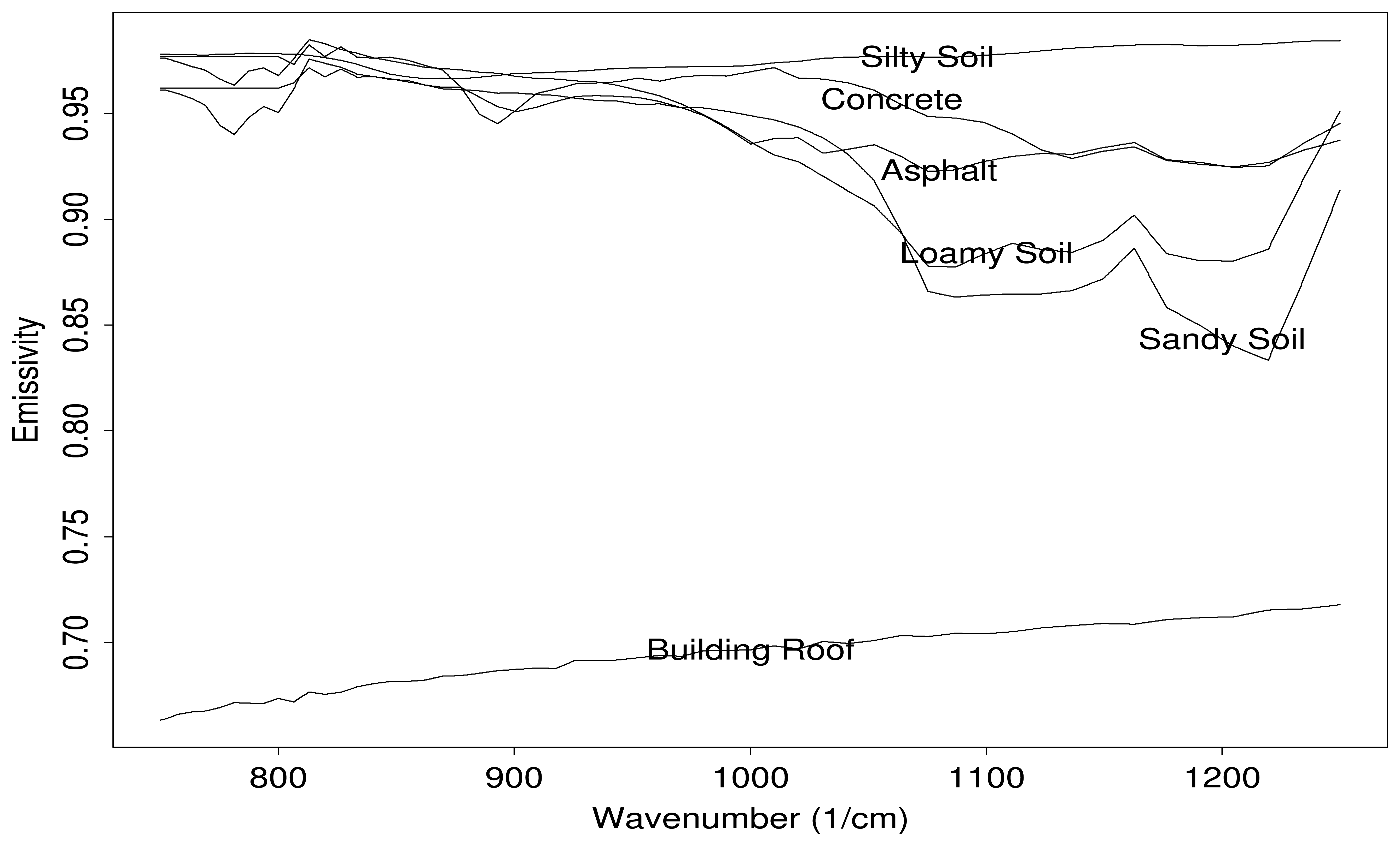
3.2. Derivation of the Prior Information

Let p(β, η) denote the prior distribution of the model parameters. Without loss of generality, the nuisance parameters can be assumed to be independent from the parameters of interest:
p ( β , η ) = p β ( β ) p η ( η )
where η = (Tg, Tp, ϵg) and β = Sensors 07 00905i2 = ( Sensors 07 00905i21,…, Sensors 07 00905i2J).
The generalized Beta distribution and the truncated Gaussian distribution with large variance are commonly used to defined weakly informative priors on large intervals [15, 16]. Using the second approach, a weak or diffuse prior for the concentrations can be formulated as follows:
p β ( β ) = C 0 [ Π j = 1 J I ( C j [ 0 , M j ] ) ] ϕ J ( C , μ c , c )
where C0 is a normalization constant so that pβ is a true distribution, I (Cj 0, Mj]) is 1 if 0 ≤ C|Mj, and 0 otherwise, and ϕJ (·,μ, ∑) denotes the J-dimensional Gaussian distribution with mean and covariance ∑. Note that the normalization constant C0 does not need to be known for the Bayesian estimation of the state parameters. By choosing Mj and ∑c large, and μc = 0, pβ slightly favors small concentration values, because most gases are likely to have zero or near zero concentration.
External information regarding the nuisance parameters is often available. For example, Tp is typically within 2 to 3K degrees of the the atmosphere, which is known from meteorological data. A prior for the background temperature Tg can be developed from scene brightness temperature, i.e., the conversion to brightness temperature from radiance using the inverse of Planck's function, and with use of the Nonconventional Exploitation Factors Data System (NEFDS), a government database of surface reflection parameters, e.g., [22] and the National Geospatial-Intelligence Agency (NGA).
Defining priors for the background emissivity is more challenging. The ground emissivity has two important properties that need to be considered in the model and the prior: smoothness and constraint to be in the interval [0, 1]. On the other hand, there is a lot of available information on ground emissivity. For example, the NEFDS database contains pre-measured surface reflection parameters for over 400 materials corresponding to a wide variety of objects ranging from camouflage to white paint. This context motivates the following approach for building a prior distribution for the ground emissivity: (1) Model the emissivity as a smooth function of the wavenumber using for example a spline function [23], (2) choose a Gaussian prior for the spline coefficients, with mean and covariance determined from the mean and covariance from the NEFDS library, and (3) map the spline function to the [0, 1] interval via a nonlinear transformation such as the logistic function: logistic(x) = (1 + exp(−x))−1.
A simpler use of the NEFDS library for defining a prior on ϵg is as follows. First, consider a sample of m emissivities corresponding to a subset of m materials in the NEFDS library. Compute the mean of this sample. Compute the singular value decomposition of the sample of centered emissivities. Let dEk denote the k-th eigenvector. Then, one can model ϵg as follows:
ϵ g = E ¯ + λ k = 1 m 1 d E k α k
where α = (α1,…,αm−1) has a Gaussian distribution with mean 0 and covariance equal to the square of the diagonal matrix of eigenvalues resulting from the singular value decomposition, and λ is a constant we set to 4 in order to generate a diffuse prior. For our experiments we used m = 6 emissivities. These emissivities were chosen to be extreme representatives of the NEFDS library, and are displayed in Figure 1.

4. Parameter Inference

Bayesian inference about the model parameters relies on their posterior distribution. Given the data model (6) and the parameter prior distribution (7), the posterior distribution π(β, η|Lobs) of these parameters is given by
π ( β , η L obs ) = C 1 exp ( 1 2 i = 1 n ( L obs ( v i ) F ( v i ; β , η ) ) 2 υ ( v i ) ) p ( β , η )
where C1 is a normalization constant. Two approaches are commonly used to construct parameter estimates and their associated uncertainties. One can either use the posterior mean and posterior covariance, or the posterior mode and highest posterior density interval.

4.1. NLMPD Algorithm

In order to produce the mode of the posterior (10), we chose a constrained version of a Levenburg-Marquardt iterative algorithm [24] we coined NLMPD for Nonlinear Maximum Posterior Density. Since the priors we used are bounded, the maximization algorithm must deal with these constraints. NLMPD is very efficient for nonlinear least-squares problems and usually converged in a few steps (3 to 10) for our problems. Thus this algorithm requires roughly 3 to 10 times the computation that a matched filter estimator would, and we can consider that they are comparable in speed. NLMPD also requires the first derivatives of the minimizing function to be known. Consequently, one can approximate, at no cost, the uncertainties associated with the mode estimate with an approximation of the posterior covariance matrix given by
post ( prior 1 + d F T E 1 dF ) 1
where ∑prior is the covariance matrix of the prior distribution, and dF is the multivariate derivative of F(v; β, η) with respect to the parameters (β, η). This approximation will produce good results when the posterior distribution is close to normal and the gas burden estimates are not highly correlated. However, when the gas burdens are highly correlated (in the posterior, not prior), the covariance approximation can be too large.

4.2. Markov Chain Monte Carlo Algorithm

Let X the candidate point is accepteddenote the model parameters. MCMC generates sequences of random variables X0, X1, X2,… that form, after a sufficiently long burn-in of say T iterations, dependent random samples of the posterior distribution π(X). Thus, any feature of the posterior distribution, including the distribution itself, can be approximated from the dependent sample [16].
The simplest MCMC is the Metropolis-Hastings algorithm [25], which, at each time t, chose the next state Xt+1 by first sampling a candidate point Y from a proposal distribution q(·|Xt). The candidate point Y is then accepted with probability
R = min ( 1 , π ( Y ) q ( X t Y ) π ( X t ) q ( Y X t ) ) .
If the candidate point is accepted, the next state become Xt+1 = Y, otherwise the chain does not move, i.e., Xt+1 = Xt. In particular, note that this algorithm does not require computation of the normalization constant C1 in (10). In most applications, C1 cannot be reliably computed as it requires a high-dimensional integration.
Remarkably, the proposal distribution q can have any form. It may also depend on the current point Xt. However, the rate of convergence of the chain to the posterior distribution, as quantified by the effective sample size of the generated sequence and its mixing will depend on how close q is to π. The effective sample size is given by the length of the sequence minus the number of rejections in (12) while the quality of the mixing is measured by the auto-correlations found in the sequence. Low autocorrelations (i.e., large mixing) produce faster convergence for the posterior estimates. We have found that an efficient proposal q for our problem is a multivariate Gaussian, centered at the current point in the sequence and with covariance equal to the covariance estimate provided by NLMPD divided by 4.
Due to the typical high-correlations observed between the effluent concentrations within the plume, the mixing remains in many cases very low. This forces us to generate very long MCMC sequences and thin them. Thinning consists of subsampling from the sequences by selecting every N-th observation. In other words, in order to produce a reliable sample of size say 5000, one need to generate first an MCMC sequence of length 5000 × N and then extract every N-th observation. As typical values of in our context is in the order of 100, generating such MCMC becomes costly.
Recently, Hamiltonian paths have been proposed to both increase the mixing in the MCMC sequence and reduce the number of rejections [17]. The Hamiltonian MCMC is built upon the basic principle of Hamiltonian mechanics. Let the function U be such that π(X) ∝ exp(−U(X)). The model parameters X can be regarded as a position vector and U(X) the potential energy function. Introducing a fictitious momentum vector P = (p1,…,pd) and mass vector M = (m1,…, md), where d denotes the number of model parameters, one can define the kinetic energy function K ( P ) = 1 2 i = 1 d p i 2 / m i. The total energy is then
H ( X , P ) = U ( X ) + K ( P ) .
Consequently, if one can sample (X, P) from the distribution π (X, P) ∝ exp(−H(X, P)), then the marginal distribution of X is exactly the target distribution π(X).
Hamiltonian dynamics allows one to move along trajectories of constant H, taking large jumps in the parameter space. The Hamiltonian algorithm alternates between picking a new momentum vector and following such trajectories. Each iteration starts with a generation of a new momentum according to a multivariate uncorrelated Gaussian distribution with (diagonal) covariance D. Then a trajectory that maintains a constant H is approximated by a discretized version, called leapfrog technique, which consists of iterating the following steps h times:
P ( t + δ / 2 ) = P ( t ) δ 2 U X X ( t )
X ( t + δ ) = X ( t ) + δ M P ( t + δ / 2 )
P ( t + δ ) = P ( t + δ / 2 ) δ 2 U X X ( t + δ )
where t denotes the t-th iteration of Hamiltonian MCMC, X (t) = Xt, P(t) denotes the momentum at the beginning of the leapfrog step, and represents a small increment.
Because the leapfrog technique is only an approximation, H may vary along these paths. A Metropolis step is then use to re-establish the equilibrium. The state at the end of the Hamiltonian path Xt+1 = X(t + ) is accepted with probability R = min(1, exp(−H(Xt+1,Pt+1) + H(Xt, Pt)) where Pt = P(t) and Pt+1 =P(t + ).
The efficiency of the Hamiltonian algorithm depends on the choices for the δ, h, M, and D. δ must be small enough to ensure that H does not change much on the approximated paths (to minimize the rejections in the Metropolis step), but it must be large enough to not slow down too much the computational time. Δ = must be large enough to ensure good mixing. M and D must be chosen to ensure that the Hamiltonian MCMC samples adequately cover the target distribution π. For our problems, we found that Δ = 0.05, h = 50, M equal to the inverse of the diagonal elements of the covariance matrix estimate given by NLMPD, and D = Diag(M0.5) produce the desired sequences.
Finally, in our context one can often expect to find parameter estimates on the distribution boundaries. For example, some gases that are part of the model are not present in the plume or are in very small concentrations. MCMC techniques, Metropolis and Hamiltonian, have difficulties generating legitimate candidates that are within the boundaries of the parameter space, leading to many rejections before a suitable candidate can be proposed. To solve this problem, we present a bouncing algorithm that conserves the equilibrium property central to the MCMC algorithm.
Let V and W denote the current and next states in the MCMC sequence. For the standard MCMC algorithm, V = Xt and W = Y, while for the Hamiltonian MCMC, V = X(t + ) and W = X(t + (g + 1)δ)) with g < h. Note that one can write W = V + ΔV, The idea is that if W lies outside the distribution boundaries, we replace it with a legitimate candidate W* in the same direction as W, i.e., W* = V + ρΔV. The algorithm mimics the physics of a ball leaving the position given by V in the direction of W, bouncing back on its path whenever it hits the boundary wall and stopping when it has traveled the distance ΔV. Note that given the boundary locations, the ending point may be between the points V and W or somewhere in the opposite direction of W, i.e., ρ may be negative.
The bouncing algorithm determines ρ as follows. Let = |ΔV| be the norm of ΔV, and A = ΔV/. Let U and L denote the upper and lower bounds of the parameter space. Compute the following quantities:
  • au ← (UV))/A and al ← (LV)/A.
  • b ← max{p min{al, au}}
  • b2 ← min{p max{al, au}}
  • bb2b1
  • ρ ← (b1) modulo 2b
  • if ρ > b then ρ ← 2bρ
  • ρ ← (ρ + b1)/
where p max{a, b} denotes the maximum taken on the vector components (p max{a, b}i = max{ai, bi}), while p min{a, b} denotes the minimum.

5. Applications

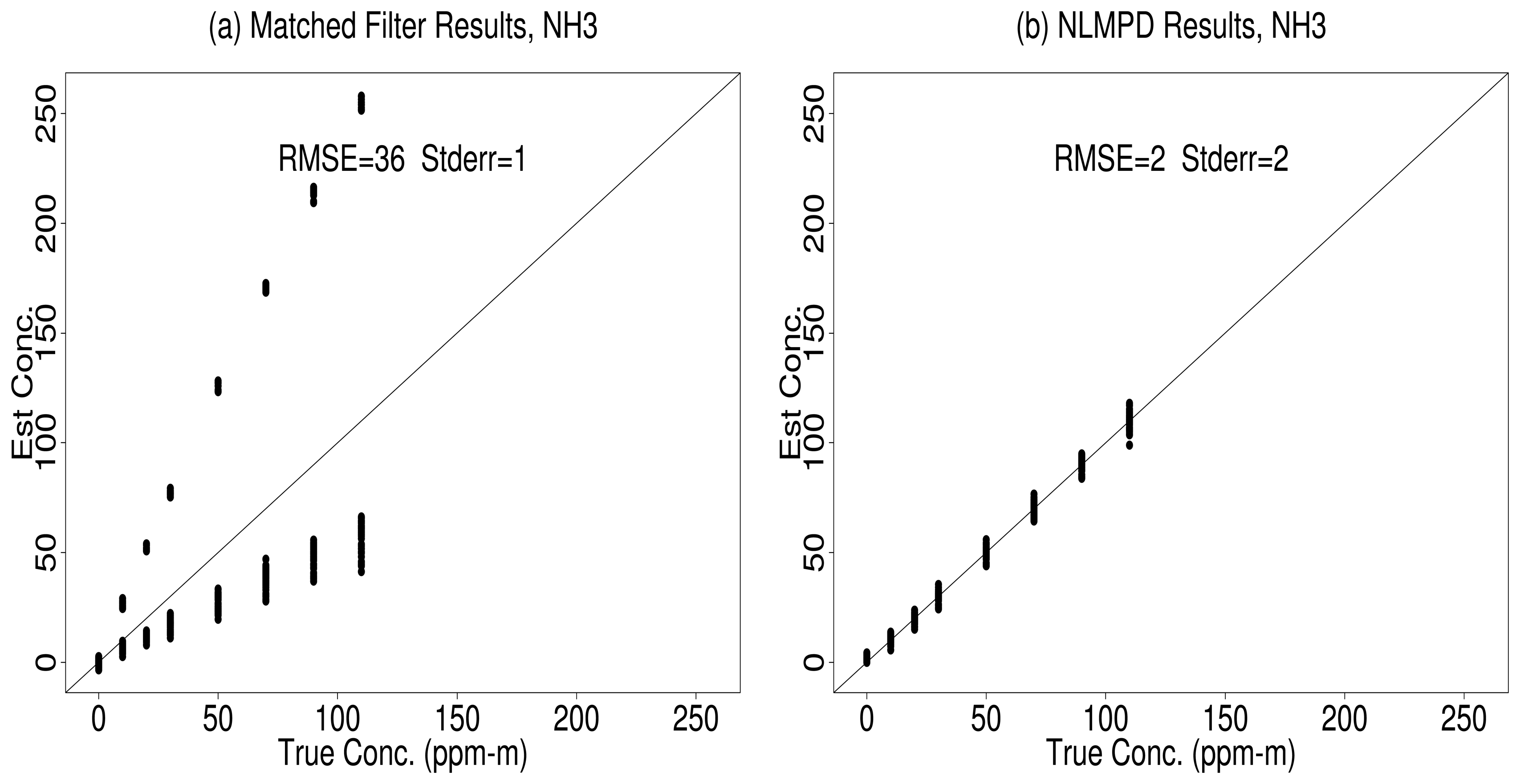
5.1. NLBR vs. Matched Filter
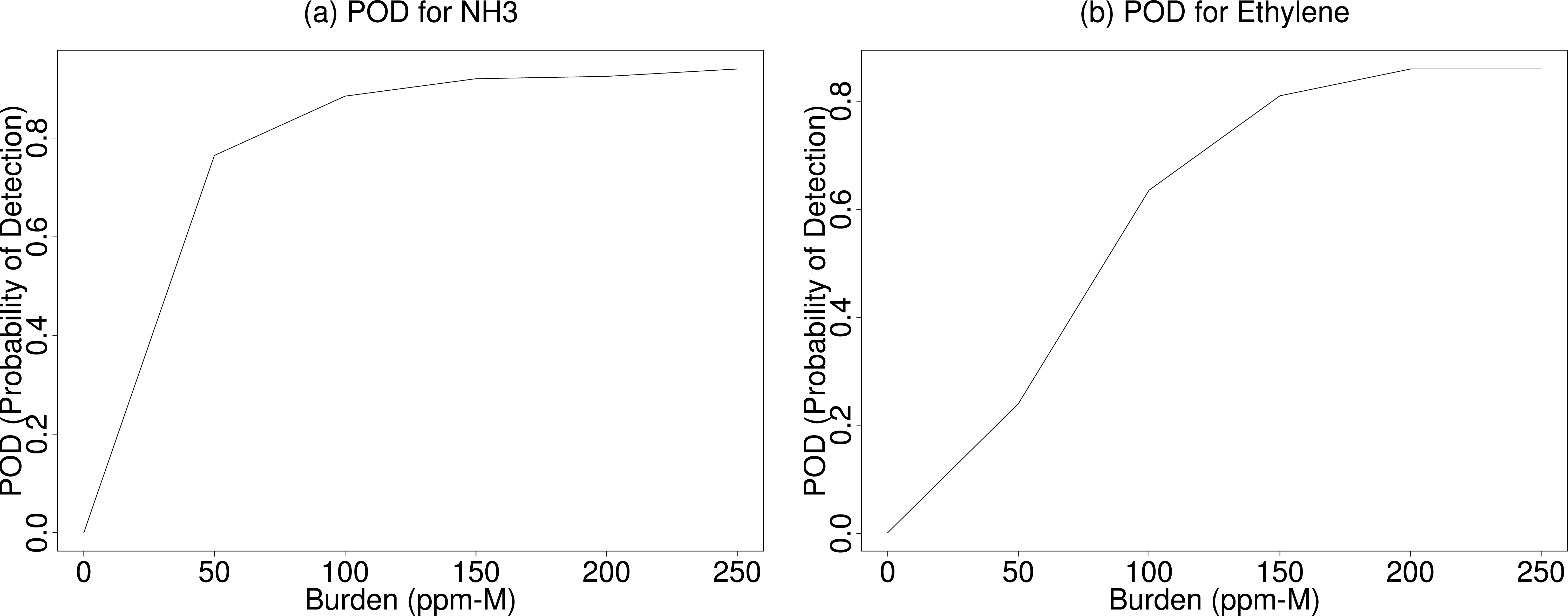
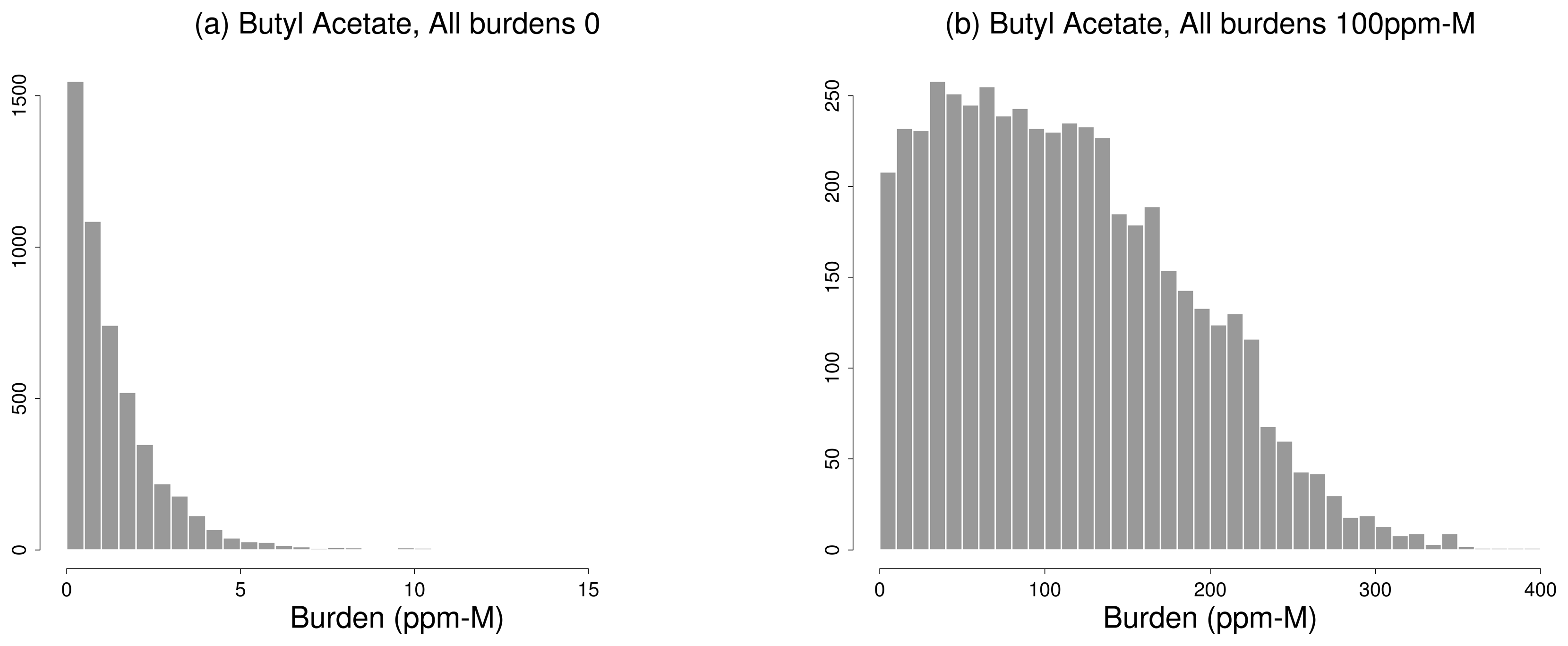
To test the methodology, we simulated spectra with known gas burdens and compared the NLBR approach with a matched filter, perhaps the most popular algorithm currently in use for gas plume detection. We considered the case of a plume with 3 non-correlated gases — NH3, Ethylene and Butyl Acetate — at various concentration levels: 0, 10, 20, 30, 50, 70, 90, and 110 ppm-M. For each level of concentration, 100 spectra were generated. For each simulation, the background emissivity was randomly selected from the 6 emissivities shown in Figure 1.
Figure 2 compares estimates of NH3 obtained with NLMPD and the matched filter. The figure plots the true burden of NH3 (horizontal axis) versus the estimates (vertical axis). Consequently, a plot for a perfect algorithm would have all the estimates on the identity line. One can see that the matched filter estimator displays much more variability than the NLBR estimator (except when the gas burden is 0). In fact, the matched-filter plot contains points that look like outliers. These “outliers” are associated with the simulations that picked an atypical background emissivity (the bottom one in Figure 1). In the linearization that the matched filter algorithm uses, an average emissivity is plugged in, which results the observed “outliers.” In the NLMPD algorithm the variability in emissivity seen in Figure 1 is accounted for in the prior.
Because of this problem, the matched-filter estimates are biased, and the actual error in the estimates (matched-filter Root Mean Squared Error RMSE=36ppm-M) is much greater than the error predicted by the algorithm (matched-filter predicted standard error=1ppm-M). On the other hand, these problems are absent from the NLBR estimator; It has no detectable bias, and the observed and predicted estimation error, given by (11), are the same (RMSE=2ppm-M, average predicted standard error=2ppm-M).

5.2. Gas Detection

The fact that the NLBR algorithm produces realistic standard errors has great benefit when the estimates are used for detection. The usual statistic to test the presence or absence (0 ppm-M) of a gas is the t-statistic, i.e., the algorithm estimate divided by the algorithm predicted standard error given by (11). Under the “null” hypothesis of no gas burden, the t-statistic should approximately follow a truncated Gaussian distribution (truncated because burdens are constrained to be non-negative).
Figure 3 presents the distributions of the t-statistic for NH3 and Ethylene, calculated from 1000 spectra simulated as in the previous example at concentration level 0 ppm-M. The distributions are presented in the form of Q-normal plots, and therefore, the t-statistic values should ideally line up on a straight line except for the truncated values. As one can see from the plots, the null distributions conform closely to the theoretical ideal.
This means that detection thresholds for NLBR estimates and the associated false call rate can be theoretically calculated and results will correspond to theory. Figure 4 presents probability of detection (POD) curves calculated from 2000 spectra, the above 1000 spectra and 200 spectra for each of the concentration levels 50, 100, 150, 200 and 250 ppm-M. Detection occurs when the t-statistic is larger than 3, a threshold that should give about a one in a thousand chance of a false call. In the figure, POD is plotted as a function of true gas concentration, so POD(0) is the false call rate. For NH3, the observed false call rate is in fact 1/1000, for Ethylene the false call rate is 3/1000, very good agreement with theory.
Fits of the NLBR model to actual hyperspectral cubes have shown that the performance shown in Figure 4 is more optomistic than that experienced on real data. For example, the residuals from real data fits are typically from 2 to 5 times larger than theory would predict, indicating that un-modeled sources of variability exist in the data. One obvious source is the atmospheric terms in the model, which are currently assumed to be perfectly known. The next step in our modeling strategy will be to construct a prior that adequately reflects variability in these terms.

5.3. Highly Correlated Gases

The results presented up to this point utilize the “quick” Bayesian solution provided by the NLMPD approach. Figure 5 presents a case for which the complete posterior, as provided by MCMC algorithm is very useful. For this example, 11 highly correlated gases were placed in the plume. The gas correlations are so large that gas burden estimation would be an ill-conditioned problem, if an unconstrained linear regression model were employed. (The principal constraint that makes this problem solvable is that all gas burdens must be non-negative). With the aid of this constraint, the Bayesian regression algorithm transforms an ill-conditioned problem to one with a very informative solution. Unfortunately, the posterior distribution for this problem is poorly approximated by a normal, and the NLMPD approach cannot provide reliable estimates. On the other hand, the MCMC algorithm can calculate the full posterior and provide critical insight on what is happening.
The two histograms in Figure 5 represent the posterior distribution for Butyl Acetate, one of the gases in the 11-gas plume. The first posterior distribution represents the estimated burden of Butyl Acetate when the true burden for each of the 11 gases is 0 ppm-M. For this case, the MCMC algorithm estimates the true burden with great accuracy even though large correlations exist between gases. In fact, a 95% highest probability density interval is (0, 4.5) ppm-M, quite a small interval. Furthermore, the MCMC output reveals that the posterior for Butyl Acetate has an exponential shape with a modal value of 0, which is far from normal.
The second posterior distribution illustrates the problem that occurs when the plume contains a large amount of the gases (100 ppm-M for each gas). In this case, the shape of the distribution is dramatically different; between 0 and 100 ppm-M it is roughly uniform, and becomes roughly normal above 100 ppm-M (or more appropriately half-normal). The uniform portion below 100 ppm-M is produced by the fact that the Butyl Acetate signal is equivalent to a linear combination of other gases. The normal half of the distribution is caused by the constraints on the linear combinations (burdens are non-negative), which become active at higher-burdens. Note that the exact nature of the correlations in the plume gases can create posteriors with quite a complex shape; It is possible to have several modes in the posterior. As one can see, the MCMC can be very valuable for evaluating plumes that may contain several gases.
The above histograms were constructed from a sample of 5000 data points generated by the Hamiltonian MCMC, after a burn-in phase of size 1000. Similar outputs could be obtained with the “traditional” MCMC algorithm described in Section 4.2, using a thinning of size N = 100. In other words, the second MCMC algorithm had to generate first a sequence of length 600,000, the first 100,000 being used for the burn-in phase, and then extract each 100′th observation to build the final sample. Because of this very high thinning, the “slow” Hamiltonian MCMC turned out to be faster by a factor of 2 than the traditional MCMC algorithm. Note that in less correlated experiments as the examples discussed earlier, the two algorithms were found to be comparable in speed.

6. Summary and Conclusions

The nonlinear Bayesian regression shows definite promise for producing better estimates from hyper-spectral data. To be most useful, NLBR should not be considered to be a specific algorithm, derived from a specific model, but a general framework for producing estimates that can be tailored to the problem at hand.
The effectiveness of these regression models depends heavily on the prior information supplied to them. The methodology does require that realistic prior distributions be constructed on the nuisance parameters. However, the fact that uncertainties can be incorporated into the prior distributions in a straightforward manner means that the Bayesian methodology incorporates these uncertainties in a fairly automatic way. In fact, one of the strongest motivations for using a Bayesian models may be because its statements of estimate uncertainty are more believable than those from other methodologies.
Our simulations involving NLBR have produced results that correspond with theory. The application of the present NLBR model to real hyper-spectral data have produced less optimal performance; It is obvious that real hyper-spectral data contains more variability than our NLBR currently describes, most prominently, atmospheric variability [26]. However, the flexibility of the NLBR framework should allow us to include these other sources of variability without any dramatic change in the general approach.

Acknowledgments

The authors would like to acknowledge the helpful advice of Herb Fry, Tom Burr, Bernie Foy, and Brian McVey of Los Alamos National Laboratory. This work was supported by the Computational and Information Science Initiative at the US Department of Energy's Pacific Northwest National Laboratory, Richland WA 99352. Pacific Northwest National Laboratory is operated by Battelle Memorial Institute for the US Department of Energy under Contract DE-AC05-76RL01830.

References

  1. Funk, C.C.; Theiler, J.; Roberts, D. A.; Borel, C. C. Clustering to improve matched filter detection of weak gas plumes in hyperspectral thermal imagery. IEEE Trans. Geosci. and Remote Sensing 2001, 39, 1410–1420. [Google Scholar]
  2. Young, S. J. Detection and quantification of gases in industrial-stack plumes using thermal-infrared hyperspectral imaging. Aerospace Report ATR-2002(8407)-1 2002. [Google Scholar]
  3. Messinger, D. Gaseous plume detection in hyperspectral images: a comparison of methods. Proceedings of SPIE'04; 2004; pp. 592–603. [Google Scholar]
  4. ODonnell, E.; Messinger, D.; Salvaggio, C.; Schott, J. Identification and detection of gaseous effluents from hyperspectral imagery using invariant algorithms. Proceedings of SPIE'04; 2004. [Google Scholar]
  5. Theiler, J.; Foy, B.; Fraser, A. Characterizing non-gaussian clutter and detecting weak gaseous plumes in hyperspectral imagery. Proceedings of SPIE'05; 2005; pp. 182–193. [Google Scholar]
  6. Pogorzala, D. Gas plume species identification in LWIR hyperspectral imagery by regression analyses. PhD thesis, Rochester Institute of Technology, 2005. [Google Scholar]
  7. Hernandez-Baquero, E. D.; Schott, J. R. Atmospheric compensation for surface temperature and emissivity separation. Proceedings of the SPIE'00 Aerosense, Orlando, FL; 2000. [Google Scholar]
  8. Borel, C. C. Recipes for writing algorithms for atmospheric corrections and temperature/emissivity separations in the thermal regime for a multi-spectral sensor. Proceedings of the SPIE'01 Aerosense, Orlando, FL; 2001. [Google Scholar]
  9. Borel, C. C. Artemiss - an algorithm to retrieve temperature and emissivity from hyper-spectral thermal image data. Proceedings of the 28th Annual GOMATech Conference, Hyperspectral Imaging Session, Tampa, FL; 2003. [Google Scholar]
  10. Yang, Z. L.; Tse, Y. K.; Bai, Z. D. On the asymptotic effect of substituting estimators for nuisance parameters in inferential statistics; Technical report; Singapore Management University, School of Economics and Social Sciences, 2003. [Google Scholar]
  11. Lancaster, T. Orthogonal parameters and panel data. Review of Economic Studies 2000, 69, 647–666. [Google Scholar]
  12. Realmuto, V. J. Separating the effects of temperature and emissivity: Emissivity spectrum normalization. Proceedings of the 2nd TIMS Workshop, JPL Publications; 1990; 99-55, pp. 31–35. [Google Scholar]
  13. Milman, A. S. Mathematical Principles of Remote Sensing: Making Inferences from Noisy Dat.Taylor & Francis: New York, first edition; 2000. [Google Scholar]
  14. Burr, T.; McVey, B.; Sander, E. Chemical identification using bayesian model selection. Proceedings of 2002 Spring Research Conference on Statistics in Industry and Technology; 2002. [Google Scholar]
  15. Gelman, A.; Carlin, J. B.; Stern, H. S.; Rubin, D. B. Bayesian Data Analysis.; Chapman & Hall: London, 1995. [Google Scholar]
  16. Gilks, W. R.; Richardson, S.; Spiegelhalter, D. J. Markov Chain Monte Carlo.; Chapman & Hall: London, 1996. [Google Scholar]
  17. Hanson, K. M. Markov chain monte carlo posterior sampling with the hamiltonian method. Proceedings of SPIE Vol. 4322, Medical Imaging: Image Processing; Sonka, M., Hanson, K. M., Eds.; 2001. [Google Scholar]
  18. Alder, B.; Wainwright, T. Studies in molecular dynamics i, general method. Journal of Chemical Physics 1959, 31(2), 459–466. [Google Scholar]
  19. Berk, A.; Acharya, P. K.; Bernstein, L. S.; Anderson, G. P.; Chetwynd, J. H.; Hoke, M. L. Reformulation of the modtran band model for higher spectral resolution. Proceedings of SPIE Vol. 4049, Algorithms for Multispectral, Hyperspectral, and Ultraspectral Imagery VI; Shen, S., Descour, M., Eds.; 2000. [Google Scholar]
  20. Beer, R. Remote Sensing by Fourier Transform Spectrometry.; Wiley Interscience: New York, 1991. [Google Scholar]
  21. Flanigan, D. F. Prediction of the limits of detection of hazardous vapors by passive infrared with the use of modtran. Applied Optics 1996, 35, 6090–6098. [Google Scholar]
  22. Westlund, H. B.; Meyer, G. W. A brdf database employing the beard-maxwell reflection model. Proceedings of Graphics Interface 2002; 2002. [Google Scholar]
  23. Bartels, R. H.; Barsky, B. A.; Beatty, J. C. An Introduction to Splines for Use in Computer Graphics and Geometric Modellin.; Morgan Kaufman: Los Altos, CA, 1987. [Google Scholar]
  24. Marquardt, D. M. An algorithm for least squares estimation of nonlinear parameters. J. Soc. Ind. Appl. Math. 1963, 11, 431–441. [Google Scholar]
  25. Hastings, W. K. Monte carlo sampling methods using markov chains and their applications. Biometrik 1970, 97–109. [Google Scholar]
  26. Miller, B.; Messinger, D. The effects of atmospheric compensation upon gaseous plume signatures. Proceedings of SPIE'05; 2005. [Google Scholar]
Figure 1. Emissivities of materials used in the simulations.
Sensors 07 00905f1
Figure 2. Matched-Filter Estimator Compared to NLBR Estimator.
Sensors 07 00905f2
Figure 3. Q-normal Plots of the T-statistic for NH3 and Ethylene, When the True Gas Burden is 0.
Sensors 07 00905f3
Figure 4. POD Curves for NH3 and Ethylene.
Sensors 07 00905f4
Figure 5. MCMC Derived Posterior for a Plume with 11 Highly Correlated Gases.
Sensors 07 00905f5

