1. Introduction
Sea surface wind is a key parameter for the exchanges of heat and moisture between sea and atmosphere [
1]. The sensitivity of polarimetric microwave radiometric observations to the wind vector has been demonstrated by several aircraft experiments (e.g. [
2]). With respect to the scatterometers, a polarimetric radiometer has the additional capability of retrieving further sea (e.g. surface temperature) and atmospheric variables (e.g. water vapor). The WindSat radiometer [
3], launched in 2003 aboard the Coriolis satellite, presently provides polarimetric passive measurements for retrieving the sea surface wind vector. It is a multifrequency instrument operating at 6.8, 10.7, 18.7, 23.8, and 37.0 GHz. The 10.7, 18.7, and 37.0 GHz channels are fully polarimetric, while 6.8 and 23.8 GHz channels are vertically and horizontally polarized.
Modeling the polarimetric microwave signature of the sea surface emission is essential for wind vector retrieval. A huge amount of studies, both theoretical and experimental, have been devoted to sea surface emission and scattering. A model of sea emission can be based on scattering models through the application of the Kirchoff's law. The Two-Scale Model (TSM) [
4] is probably the most widely used method to generate synthetic satellite passive polarimetric observations, i.e., to simulate the modified Stokes vector (
TB), whose components are the brightness temperatures at vertical (
TBv) and horizontal (
TBh) polarizations, and the correlation parameters (
U and
V), emitted and scattered by a marine surface. Although several alternative methods have been developed, such as the Small Slope Approximation [
5], it has not yet demonstrated that one method is superior with respect to the others [
6].
In previous investigations, we have developed and validated a software package (named SEAWIND) based on the TSM and capable to simulate the fully polarimetric microwave passive observations of a spaceborne radiometer [
7,
8]. This package has been recently improved and updated to produce synthetic backscattering coefficients as well (and its current name is SEAWIND2, hereafter denoted as SW2) [
9]. In another study [
10], which considered the WindSat polarimetric channels, we have exploited the universal approximation property of Neural Networks (NN's) to emulate the TSM, thus dealing with the problem of its low computational efficiency, which makes its use difficult to employ iterative techniques to solve the inverse problem.
The objective of this work, which basically represents the continuation of [
10], is the investigation of the use of the NN's developed in [
10] to tackle the inversion problem. In [
10], the NN's have been trained to match the input-output relationship of the TSM (input: geophysical parameters; output:
TB). Here, we use the trained NN's to find the wind vector which best accounts for the measured
TB. To our knowledge, this is the first attempt to carry out an inversion of a NN-based forward model to estimate the wind field from polarimetric microwave radiometer data. Empirical geophysical model functions have been employed, as forward models, for this purpose in [
1] and [
11], while physically-based forward model functions have been exploited in [
12] and [
13]. Note that, in [
10], we have demonstrated that Neural Networks (NN's) reproduce the behavior of the TSM fairly well, generally improving the accuracy achievable with a standard model function approach, so that an improvement on the quality of the retrieval, at least with respect to physically-derived model functions, can be expected.
To yield a reliable evaluation of the potentiality of the proposed approach for wind vector retrieval, particular attention is paid to the algorithmic aspects. Different Bayesian techniques [
14,
15], such as Minimum Variance (MV), Maximum Likelihood (ML) and Maximum Posterior Probability (MAP) criteria have been used. Furthermore, for the latter two methods, an iterative inversion of the trained NN-based forward model has been performed and different methods to minimize the cost function, such as the common Gradient Descent and the more sophisticated Simulated Annealing, have been used.
In this work we present also a method, based on an evaluation of the curl and of the divergence of the wind vector, to deal with the non-uniqueness of the wind vector solution. To analyze the potentiality of this procedure, which can represent an alternative, or a complement, to the median filtering, commonly used for processing WindSat retrievals (e.g. [
12]), a case study is considered.
The inversion techniques have been tested on simulated WindSat measurements generated by means of SW2, which has been applied to a set of meteorological analysis fields obtained from the European Centre for Medium-Range Weather Forecasts (ECMWF), collected throughout the first ten days of each month of year 2000 over the Mediterranean Sea. From such fields, whose spatial resolution is 0.5° both in latitude and in longitude, we have extracted the vertical profiles of temperature, pressure and relative humidity, as well as the surface value of sea temperature and wind velocity.
The work is organized as follows. Section 2 describes the procedure that we have adopted to retrieve the wind vector from the ECMWF-derived simulated TB's, as well as the proposed ambiguity selection technique. Section 3 is focused on the discussion of the results, while section 4 draws the main conclusions.
2. Wind vector retrieval
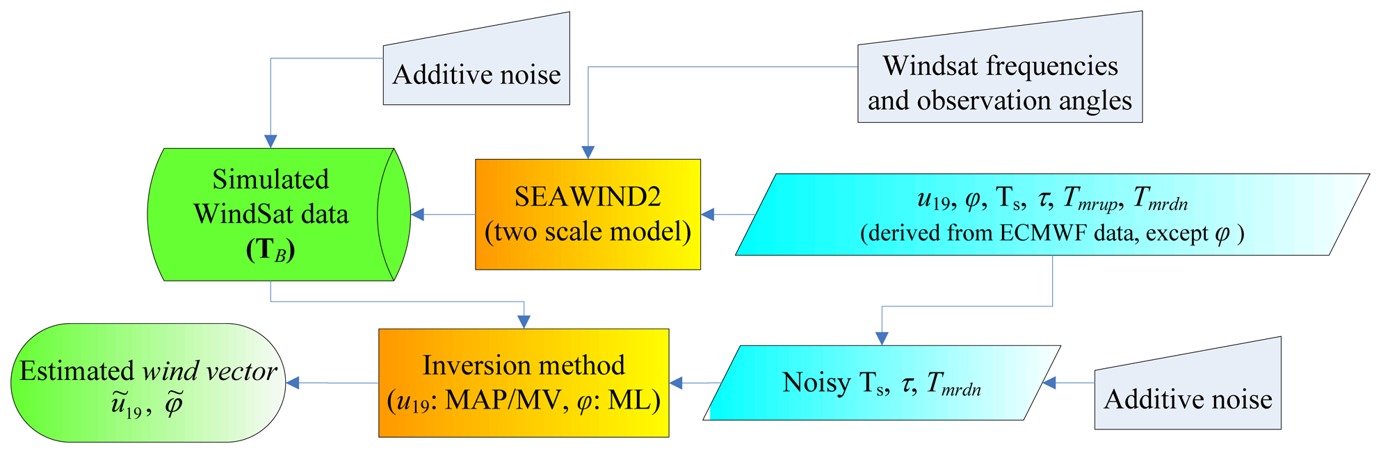
The block diagram describing the procedure we have followed to test the retrieval algorithms is shown in
Figure 1. The WindSat measurements have been simulated by running the SW2 software implementing the TSM. The inputs of SW2 are: azimuth angle between wind and radiometer pointing directions (
φ), wind velocity at 19.5 m above sea level (
u19), sea surface temperature (
TS), atmospheric optical thickness (
τ) and mean radiative temperatures (downwelling:
Tmrdn and upwelling:
Tmrup). As mentioned, these variables have been derived from the ECMWF analysis fields collected throughout year 2000, except for
φ which has been randomly generated (with uniform distribution between 0° and 360°, in the absence of any a priori information). Atmospheric radiative parameters have been computed by applying a radiative transfer algorithm to the meteorological data, namely to the vertical profiles of pressure, temperature and relative humidity, assuming the presence of clear sky, or non-precipitating clouds [
8]. To account for measurement noise and forward model errors, an additive Gaussian noise with zero mean and standard deviations equal to those found in [
12] for the different WindSat channels has been added to the SW2-derived
TB's.
ECMWF provides wind speed at 10 m of height, but the wave spectrum developed in [
9] requires
u19, so that SW2 has
u19 as input parameter. The conversion has been carried out in two steps. Firstly, we have inverted the relationship used in [
4], in which a neutral stability assumption is done, which allows the computation of the wind velocity at any height as a function of wind friction. In this way the wind speed at 10 m has been transformed in friction velocity. Then, the relationship has been applied to derive the wind velocity at 19.5 m. Hereafter, for ECMWF
u19 we will intend the wind speed computed in this way.
Focusing on the wind vector, we have assumed that columnar cloud liquid and columnar water vapor in the atmosphere, as well as
TS, have been already estimated by a separate algorithm. In the literature, several algorithms are available, such as the Ocean Algorithm for the Advanced Microwave Scanning Radiometer (AMSR) proposed in [
16], where the expected retrieval accuracies for cloud liquid, water vapor and
TS were foreseen equal to 0.02 mm, 1 mm and 0.5 K, respectively. To take into account the estimation error for
TS, an additive Gaussian noise with zero mean and standard deviation of 0.5 K has been added to this variable. From the expected estimation errors for the atmospheric parameters, the uncertainties on
τ and
Tmrdn have been evaluated through the relationships found in [
16]. Note that
Tmrdn is the only mean radiative temperature used as NN's input, because
Tmrdn and
Tmrup are strongly correlated [
10]. For
τ, we have added a random Gaussian noise with zero mean and a standard deviation equal to the 10% of the average value of the ECMWF-derived
τ. For
Tmrdn, we have added a random Gaussian noise with zero mean and a standard deviation equal to the 1% of the average value of ECMWF-derived
Tmrdn.
According to the scheme reported in
Figure 1, the “noisy”
TS,
τ and
Tmrdn, as well as the vector of synthetic measurements
TB, are supplied to the block which accomplishes the inversion, producing the estimated wind velocity
ũ19, and the estimated azimuth angle
φ̃. The components of this block are described in the following sections. The inversion is performed in 3 steps. In the first step, the wind speed is retrieved and a fixed value of
φ is used (180°). Successively, the azimuth angle is estimated through a ML criterion. Finally, the wind speed retrieval is refined by using
φ̃ instead of 180°.
The Bayesian theory of parameter estimation [
14,
15] has been considered in this work to infer
u19 and
φ. It focuses on the probability density function (pdf)
p (
x|
Y) of a certain parameter
x conditioned to the vector of measurements
Y. By applying the Bayes theorem,
p (
x|
Y) is given by:
The criteria to estimate
x may be different, depending on the cost associated to the errors of the estimation. We have used either MV or MAP criteria for wind velocity retrieval, while
φ̃ has been determined by means of a ML criterion.
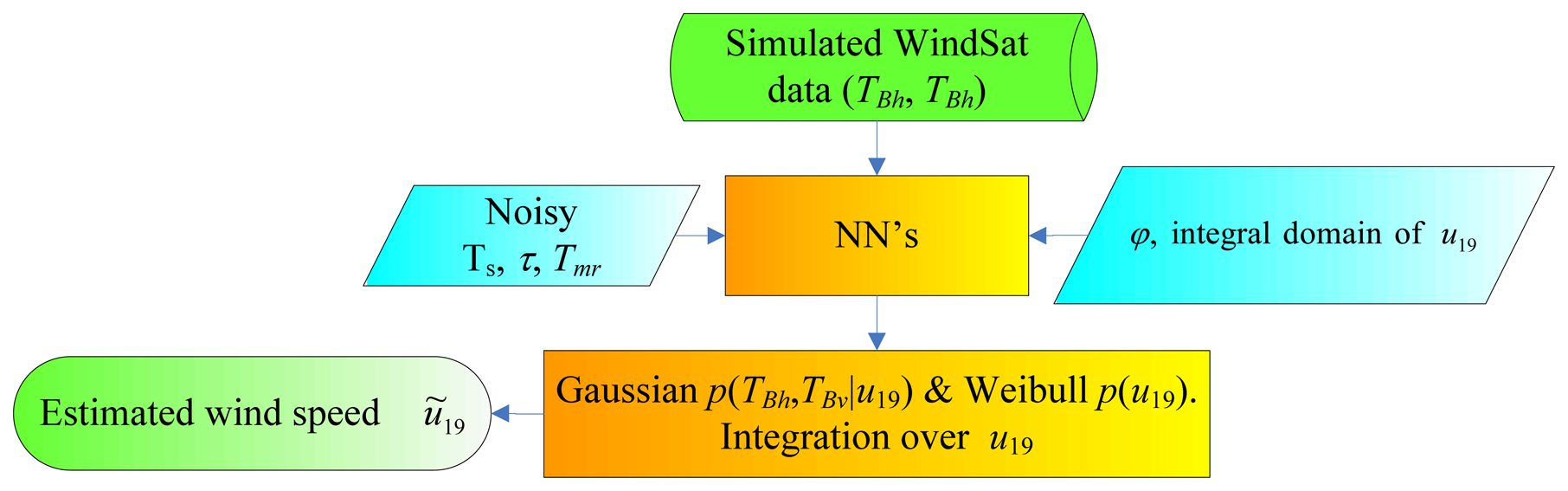
2.1. MV-based wind speed retrieval
The block diagram of the MV wind speed estimator is shown in
Figure 2. Only the first two components of the modified Stokes vector, i.e.,
TBh and
TBv, are used (as done in several papers, e.g. [
1], [
11]), since
U and
V are mainly sensitive to wind direction. The 6 GHz channels are not exploited.
The NN's block consists of four networks, one for each frequency included in the inversion process (i.e. 10, 18, 23 and 37 GHz). With respect to those developed in [
10], in which only the fully polarimetric channels have been considered, a new NN for the 23 GHz band has been built, having the same architecture and the same learning method (Bayesian Regularization) of the other networks. Using
TBh and
TBv, only the corresponding two outputs of the NN's are delivered to the estimator.
It is well known that, if we compute the expected value of
p(
u19|
Y) we obtain a MV estimator, which minimizes the root mean square (rms) retrieval error (and is also called Minimum Mean Square Estimator) [
14,
15]. The wind speed estimate is therefore given by:
where
Y=[
TBh10TBv10TBh18TBv18TBh23TBv23TBh37TBv37]
T (superscript
T indicates transposition) and
D is the integral domain of
u19, that we have chosen equal to [0-25 m/s], thus assuming that the pdf of wind speed
p(
u19) is zero outside this interval. Moreover, we have considered that
p(
Y) is obtained by saturating the joint probability
p(
Y,
u19) =
p (
Y|
u19)
p (
u19).
While
p (
Y|
u19) has been supposed Gaussian, for
p (
u19) a Weibull distribution has been assumed [
17], so that:
In
Equation (3), det(·) is the determinant,
Y(
u19) represents the output of the NN's based forward model, while
Ymeas denotes the measurements vector and
CY is the covariance matrix that should account for both measurements and forward model errors. We have assumed
CY diagonal and its elements have been taken as those provided in [
12]. For
p(
u19), the scale parameter
c and the shape parameter
k have been estimated from the ECMWF data used in this work through the ML formula suggested in [
17], finding
c=6.2889 m/s and
k=2.2054.
To compute the estimate, i.e. the integrals at the third member of
equation (2), a trapezoidal rule has been applied, sampling the domain
D in intervals of 0.05 m/s.
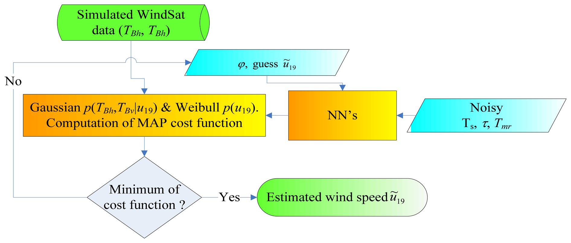
2.2. MAP-based wind speed retrieval
If, instead of computing the expected value of
p(
u19|
Y), we determine its maximum, a MAP criterion is applied. It is worth noting that, since the Weibull distribution is not a symmetric pdf, the MAP estimate differs from the MV one. Using the pdf s represented by
equations (3) and
(4), the MAP criterion reduces to minimize the following cost function with respect to
u19 [
14,
15]:
Figure 3 shows the block diagram of the MAP wind speed estimator. The minimization has been carried out through an iterative procedure, thus accomplishing an iterative inversion of a trained NN-based forward model, as proposed in [
18]. Two optimization techniques have been used, both starting from a first guess equal to the mean value of the ECMWF
u19. Besides the conventional Gradient Descent (GD) method (adopted in [
1]), a stochastic advanced method such as Simulated Annealing (SA) has been employed too. A description of the routines implementing these techniques can be found in [
19]. According to the selected algorithm, a new guess value for
u19 is produced and the NN-based forward model generates the corresponding
Y(
u19).
GD evaluates both the cost function and its gradient, basing on the idea that the direction of the negative gradient indicates where the minimum of the cost function is placed. According to this direction, another point, where cost function and gradient are evaluated, is selected and the new gradient identifies the new direction of the minimum. The iterations end when a (local) minimum of the cost function is found. GD is strongly dependent on the first guess.
As opposed to GD, SA is a global optimization algorithm. It associates to each point of the domain in which the minimum of the cost function is searched, a state of a physical system characterized by an internal energy. The minimum of the cost function corresponds to a state with the minimum possible energy. At each step of the optimization, SA considers some neighbors of the current state, randomly generated by perturbing the current state itself. Then, SA decides whether accepting or rejecting the new configuration basing on the difference between its energy and the previous one. If the energy of the new state is smaller than the original one, the new state is accepted, otherwise it is accepted with a probability depending on the Boltzmann statistics. The procedure ends when the system reaches a state that is good enough for the application, or when computational time reaches the maximum fixed by the user.
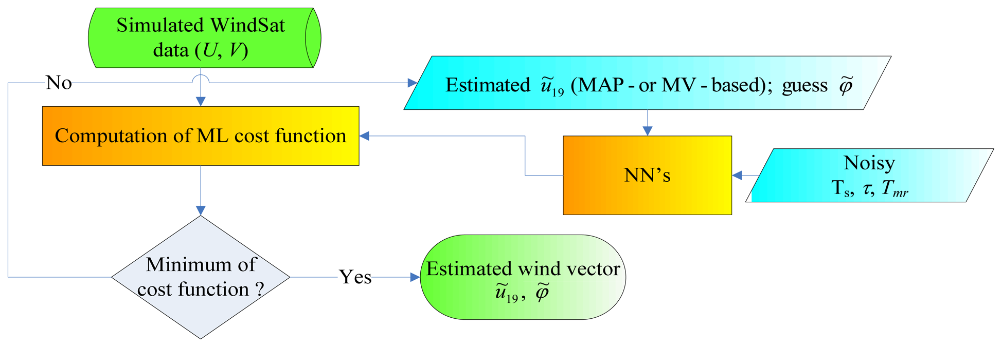
2.3. ML-based wind direction retrieval
The wind direction is identified by the azimuth angle
φ=
φr−
φw, where
φr is the radiometer pointing direction and
φw is the wind direction. The block diagram of the ML wind direction estimator is shown in
Figure 4. It uses the third and fourth components of the modified Stokes vector, i.e.,
U and
V of the fully polarimetric WindSat bands (10, 18 and 37 GHz). The choice of a ML estimator is related to the assumption of a uniform distribution for
φ. The cost function to be minimized is given by:
where
Y=[
U10V10U18V18U37V37]
T and, also in this case, the error covariance matrix
CY as been assumed diagonal with elements taken as those found in [
12]. The wind velocity supplied as input to the NN's is that estimated in the first step of our wind field retrieval procedure. Also for the minimization of
dML an iterative technique, based on the two optimization methods introduced above, has been accomplished.
It is well known that, when dealing with the retrieval of wind direction, the problem of the non-uniqueness of the solution is fairly significant. The cost function may have many local minima and different solutions (generally indicated as ambiguities) can be obtained depending on the first guess value of
φ̃ (hereafter denoted as
φ̃fg) [
1], [
11,
12]. We have searched for the four ambiguities, as done in [
12], so that the procedure illustrated in
Figure 4 has been applied four times (for each
TB of the ECMWF-SW2 test set), each time using a different
φ̃fg. One value of
φ̃fg (denoted as
φ̃fg1) has been obtained by evaluating
dML every 5°, spanning the interval [0°-355°], and selecting the azimuth angle yielding the smallest
dML. The other three values of the first guess have been chosen to be
φ̃fg1+90°,
φ̃fg1+180°,
φ̃fg1+270° [
12].
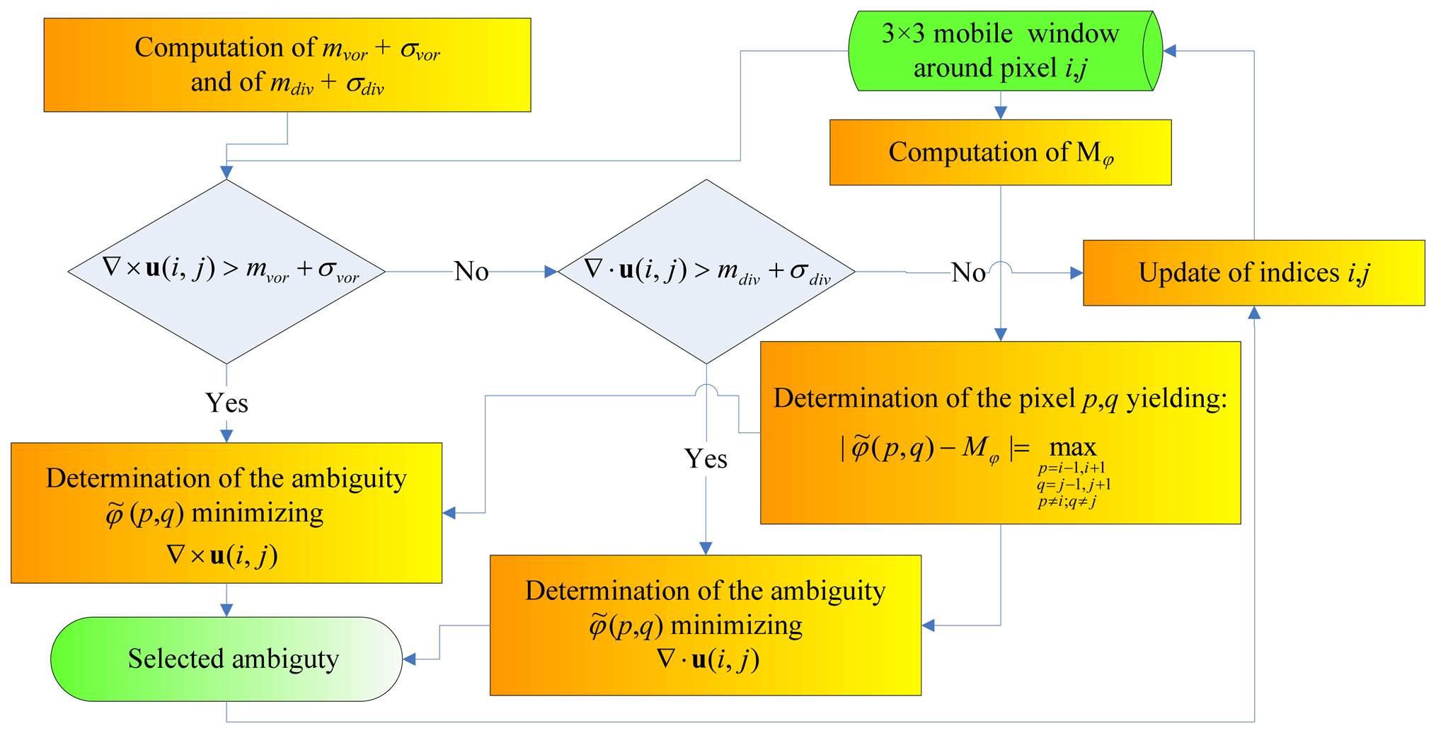
2.4. Ambiguity selection
In this section, a method to deal with the non-uniqueness of wind direction solution that exploits the contextual information by basing either on the curl of the wind vector
u (∇ ×
u), i.e., on wind vorticity, or on its divergence (∇ ·
u), is illustrated. This technique is an alternative to methods used for wind vector retrieval from WindSat that are based on median filtering [
11,
12]. The idea on which the method is based is that, in an area characterized by an unrealistic dispersion of wind directions, the norm of the vorticity and/or of the divergence is large. Selecting the ambiguity that yields the minimum value of the norm may lead to a more reliable
φ̃.
The block diagram illustrating the ambiguity selection method is shown in
Figure 5. Firstly, both the mean values and the standard deviations of |∇ ×
u| (denoted as
mvor and
σvor, respectively) and |∇ ·
u| (
mdiv and
σdiv) in the considered swath area are computed. Then, a mobile window of 3×3 radiometric pixels is considered and the median of the wind directions within the window (
Mφ) is computed. Only points presenting either |∇ ×
u|>
mvor +
σvor or |∇ ·
u|>
mdiv +
σdiv are processed. We have based the computation of the vorticity, as well as of the divergence, on the four pixels adjacent to the centre of the moving window along both the vertical and the horizontal directions. Among these four pixels, the procedure acts on that presenting the largest value of |
φ̃ − M
φ|. Then, among the four ambiguities associated to this pixel, the one yielding the minimum value of the curl or of the divergence is selected. The procedure is iterated until the wind vector ends changing its direction.
4. Conclusions
A simulation study aiming at evaluating the potentiality of a wind vector retrieval algorithm for a polarimetric radiometer, based on the approximation of the forward model by means of a NN approach, has been presented. An effort has been devoted to test several inversion algorithm, all based on the Bayesian theory of parameter estimation. In particular, MV and MAP for wind velocity, and ML for wind direction, have been considered. To minimize the cost function of both MAP and ML, a conventional technique such as GD, and a more advanced optimization method, such as SA have been employed.
The polarimetric measurements have been simulated by means of a software package, already developed and validated, implementing the two scale model. The software has been fed by data derived from the ECMWF analysis fields. The atmospheric parameters, as well as the sea surface temperature have been assumed already estimated and an uncertainty on the inputs of the NN-based forward model has been associated to the expected retrieval error of these quantities.
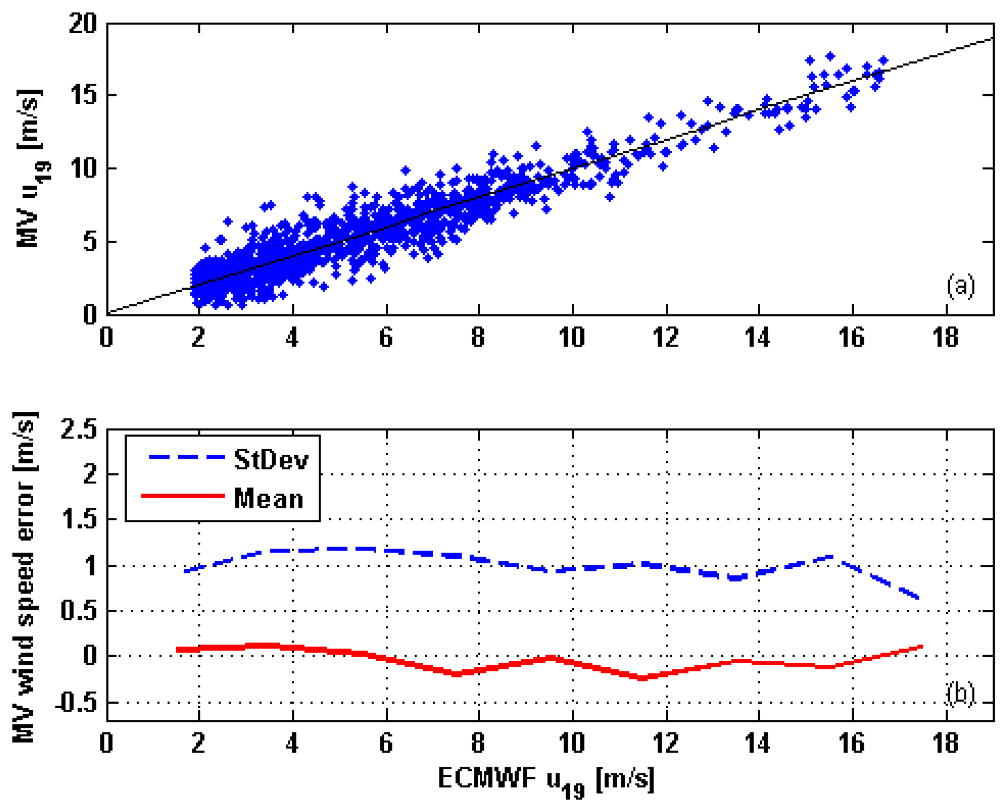
The best result for the wind speed estimation has been achieved by the MV algorithm, for which the standard deviation of the retrieval error is approximately 1.1 m/s. The performances of MAP-SA and, especially of MAP-GD are worse, although the former has the best computational efficiency.
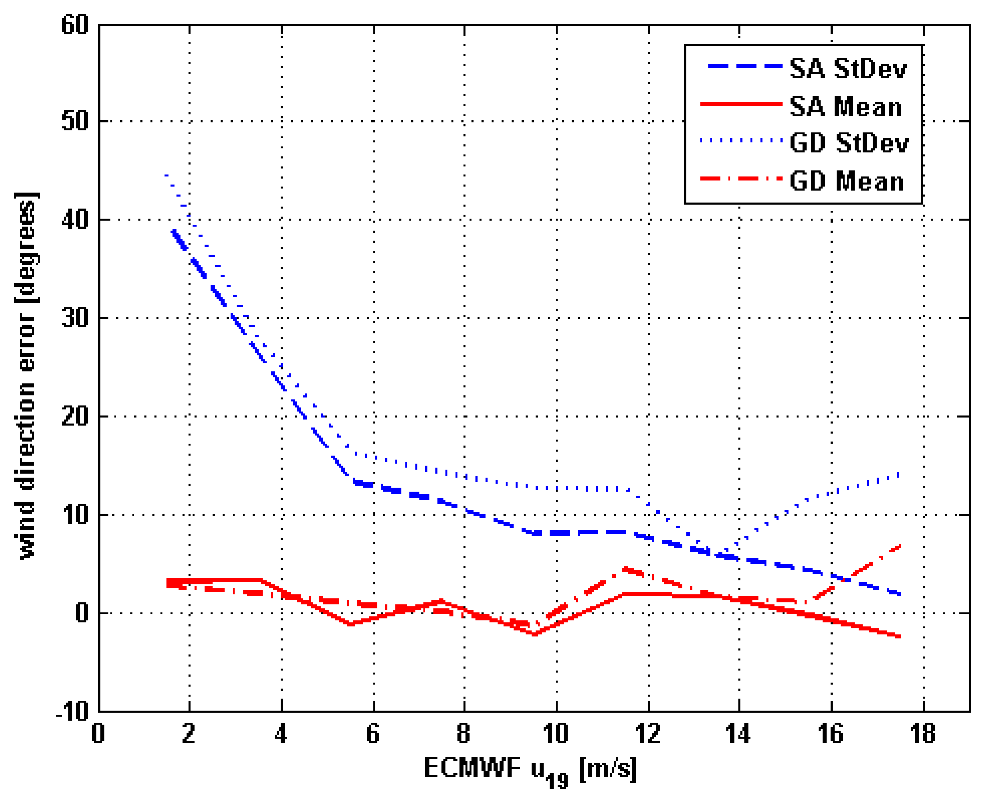
As for the wind direction, ML-SA has revealed the best estimator, yielding a standard deviation of the wind direction error for the closest ambiguity less than 13° for wind speeds larger than 6 m/s and less than 9° for wind speeds greater than 10 m/s. As already found in the literature, for lower wind velocities, the wind direction signal is weak. Moreover, we have found that the performances achieved by considering the ambiguity yielding the least value of the ML cost function are worse, so that the ambiguity selection has revealed a critical aspect.
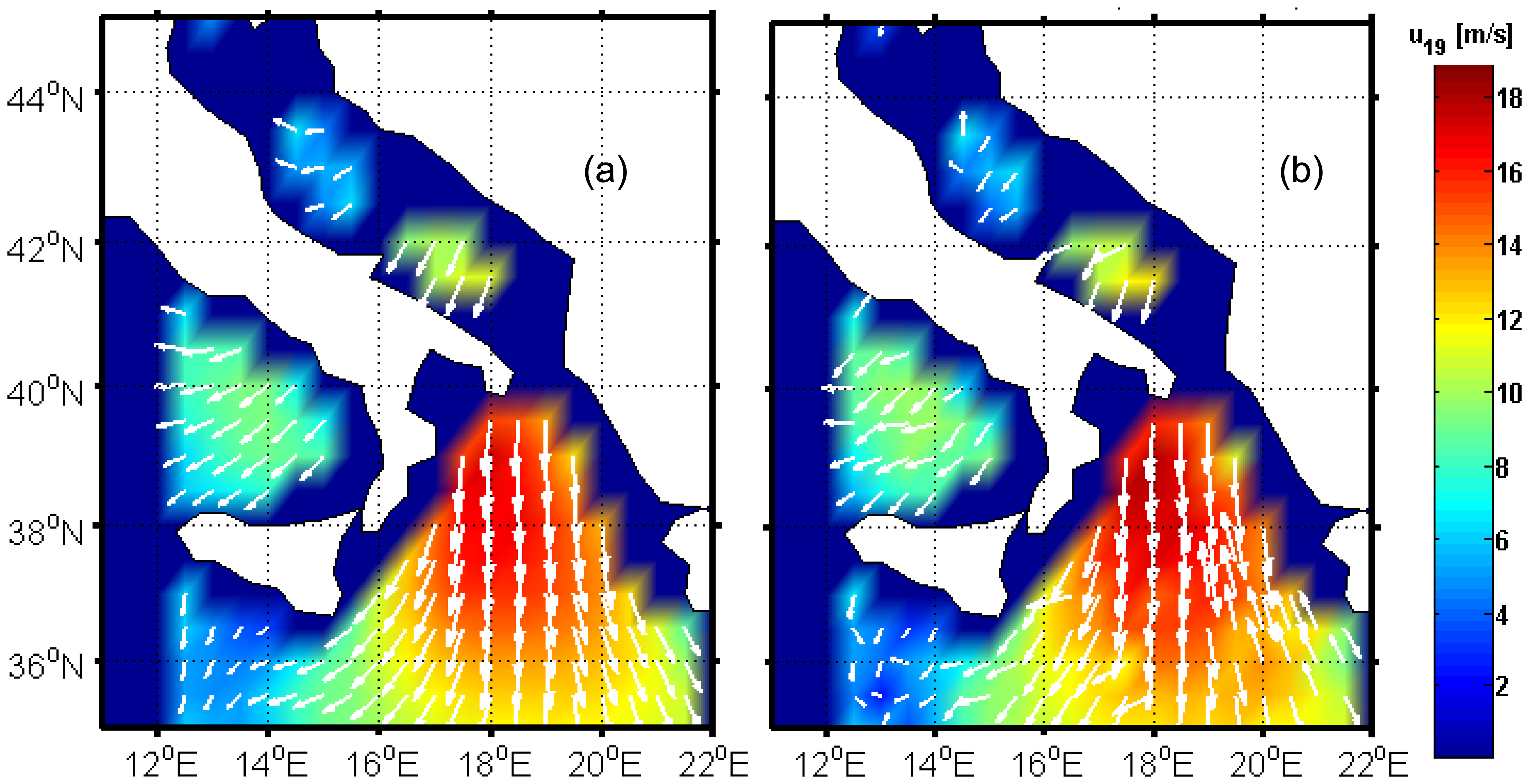
An ambiguity selection method exploiting the contextual information by basing either on the curl of the wind vector, or on its divergence, has been finally proposed to represent an alternative to median filtering used in other papers dealing with wind retrieval from WindSat data. Its application on a case study has yielded encouraging results.


