Road Asphalt Pavements Analyzed by Airborne Thermal Remote Sensing: Preliminary Results of the Venice Highway

Abstract
:1. Introduction
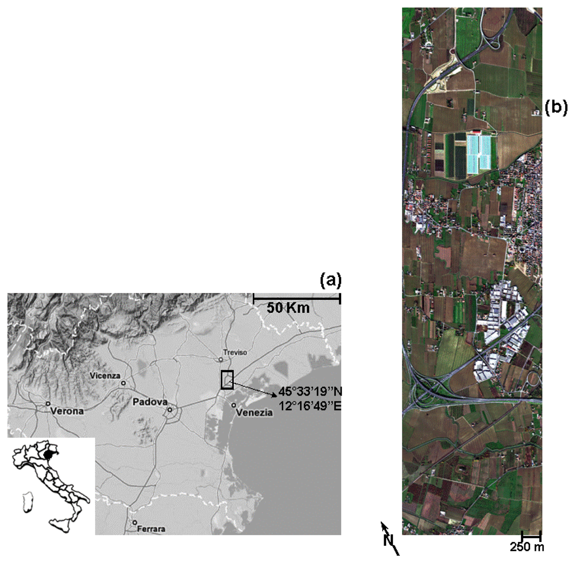
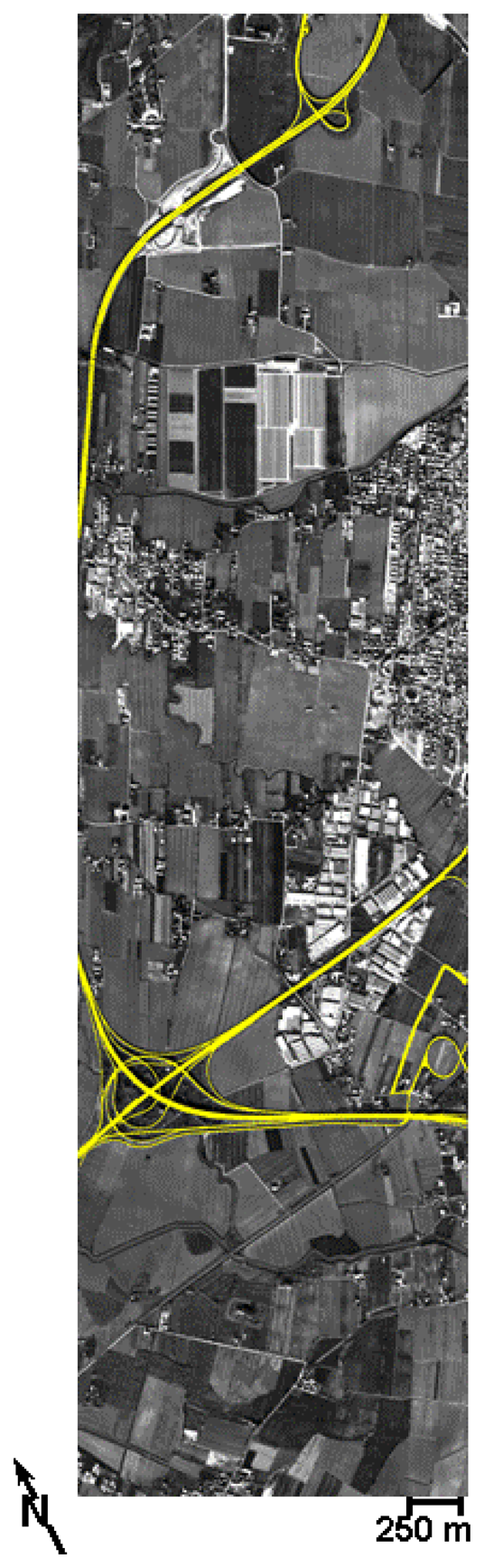
2. Study area
3. Data and methods
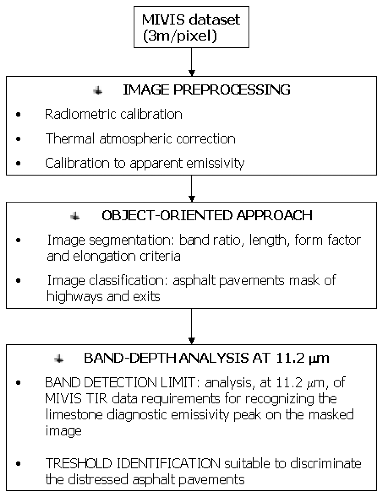
3.1. Image preprocessing
3.2. Image classification
3.2.1. Object-oriented approach
- (i)
- The “find objects” task (i.e. segmentation; [30]) that was divided, in its turn, into four steps: “segment”, “merge”, “refine”, and “compute attributes”. The “segment” and “merge” steps of this task were used to divide the image into segments corresponding to real-world objects and for solving over-segmentation problems and then the adjacent segments were grouped on the basis of their brightness value.
- (ii)
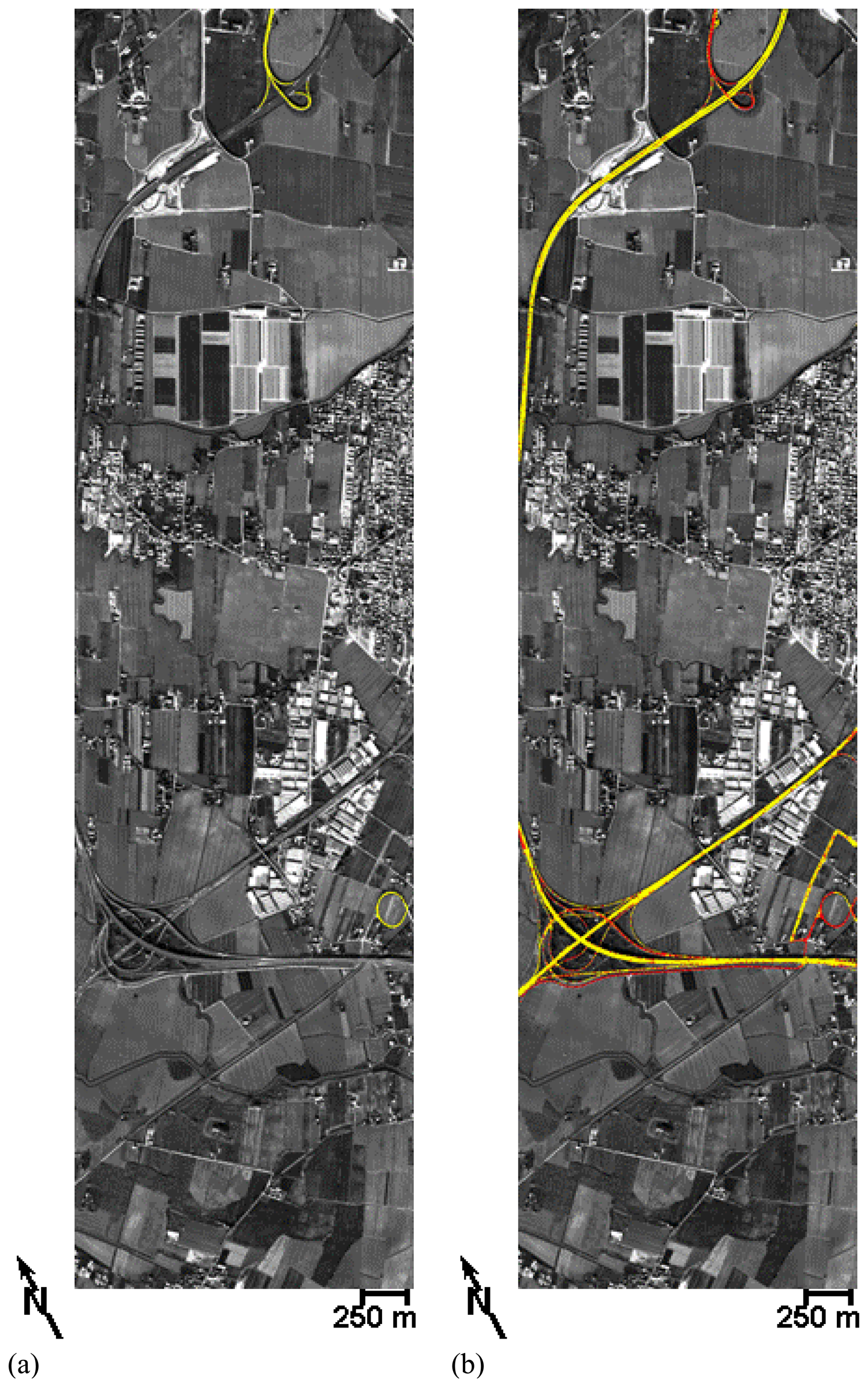
- The “rule-based classification” task (i.e. classification; [30]) was used to extract only the highways and exits objects and then to export them onto a raster image.
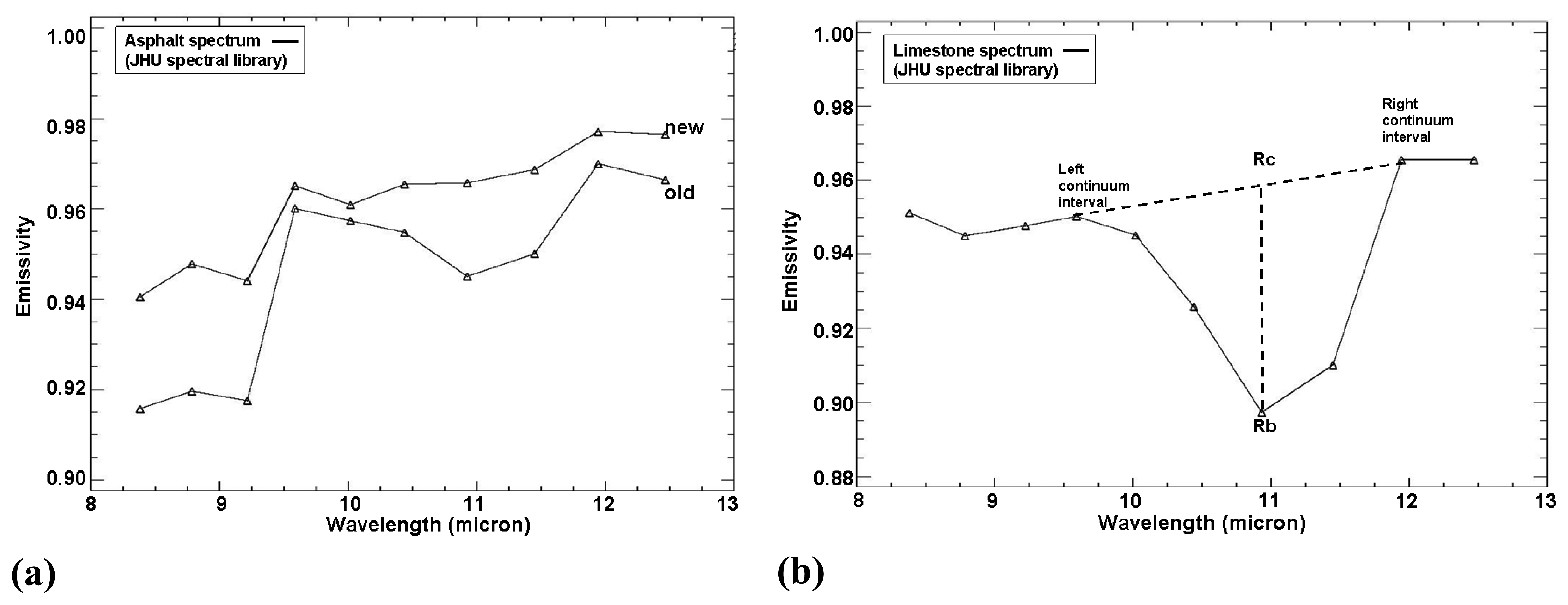
3.2.2. Band Depth analysis on asphalt roads
4. Results and discussion
4.1. Object-oriented classification results
4.2. Application requirements and Band-Depth results
5. Conclusions
Acknowledgments
References
- Bassani, C.; Cavalli, R.M.; Cavalcante, F.; Cuomo, V.; Palombo, A.; Pascucci, S.; Pignatti, S. Deterioration status of asbestos-cement roofing sheets assessed by analyzing hyperspectral data. Remote Sensing of Environment 2007, 109, 361–378. [Google Scholar]
- Bassi, P. Chimica applicata ai materiali da costruzione 1993.
- Becker, F.; Li, Z.L. Temperature-Independent Spectral Indices in Thermal Infrared Bands. Remote Sensing of Environment 1990, 32, 17–33. [Google Scholar]
- Ben-Dor, E.; Levin, N.; Saaroni, H. A spectral based recognition of the urban environment using the visible and near-infrared spectral region (0.4–1.1 m). A case study over Tel-Aviv. International Journal of Remote Sensing 2001, 22(11), 2193–2218. [Google Scholar]
- Bianchi, R.; Marino, C. M.; Pignatti, S. Airborne hyperspectral remote sensing in Italy. Proceedings of Recent Advances in Remote Sensing and Hyperspectral Remote Sensing, Rome, Italy, September 23-30; 1994; pp. 29–37. [Google Scholar]
- Boskovitz, V.; Guterman, H. An adaptive neuro-fuzzy system for automatic image segmentation and edge detection. IEEE Transactions on fuzzy systems 2002, 10, 247–262. [Google Scholar]
- Carlisle, O.; Lucey, P.G.; Sherman, S.B. Thermal infrared weathering trajectories in Hawaiian basalts: results from airborne, field and laboratory observations. Proceedings of the 37th Lunar and Planetary Science Conference, League City, Texas, March 13-17; 2006; 17. [Google Scholar]
- Clark, R.N.; Roush, T.D. Reflectance Spectroscopy: Quantitative Analysis Techniques for Remote Sensing Applications. Journal of Geophysical Research 1984, 89, 6329–6340. [Google Scholar]
- Clark, R.N.; Gallagher, A.J.; Swayze, G.A. Material absorption band depth mapping of imaging spectrometer data using the complete band shape least-squares algorithm simultaneously fit to multiple spectral features from multiple materials. Proceedings of the 3th JPL Airborne Visible/Infrared Imaging Spectrometer (AVIRIS) Workshop: JPL Publication, Pasadena, CA,, June 4-5; 1990; 90-54, pp. 176–186. [Google Scholar]
- Clark, R.N. Spectroscopy of rocks and minerals and principles of spectroscopy. In Manual of Remote Sensing. Volume 3: Remote Sensing for the Earth Sciences; Rencz, A.N., Ed.; John Wiley & Sons Inc., 1999; pp. 3–58. [Google Scholar]
- Colwell, R.N. Manual of Remote Sensing; American Society of Photogrammetry and Remote Sensing: Falls Church Eds., 1983; pp. 344–363. Volume 1196. [Google Scholar]
- CONCAWE. Bitumens and bitumen derivatives. In CONservation of Clean Air and Water in Europe (PD 92/104); Brussels, Belgium, December 1992. [Google Scholar]
- Gao, B. An operational method for estimating signal to noise ratios from data acquired with imaging spectrometers. Remote Sensing of Environment 1993, 43, 23–33. [Google Scholar]
- Gillespie, A.R.; Kahle, A.B.; Palluconi, F.D. Mapping alluvial fans in Death Valley, CA, using multispectral thermal infrared images. Geophysical Research Letters 1984, 11(11), 1153–1156. [Google Scholar]
- Gillespie, A.R. Spectral mixture analysis of multispectral thermal infrared images. Remote Sensing of Environment 1992, 42, 137–145. [Google Scholar]
- Gillespie, A.R.; Rokugawa, S.; Matsunaga, T.; Cothern, J.S.; Hook, S.; Kahle, A.B. A Temperature and Emissivity Separation Algorithm for Advanced Spaceborne Thermal Emission and Reflection Radiometer (ASTER) Images. IEEE Transactions on Geoscience and Remote Sensing 1998, 36(4), 1113–1126. [Google Scholar]
- Gillespie, A.R.; Rokugawa, S.; Hook, S.; Matsunaga, T.; Kahle, A.B. ASTER Temperature/Emissivity Separation Algorithm Theoretical Basis (Version 2.4). In Algorithm Theoretical Basis Document.; Washington, DC: NASA, Contract Number NAS5-31372; 1999. [Google Scholar]
- Gu, D.G.; Gillespie, A.R.; Kahle, A.B.; Palluconi, F.D. Autonomous Atmospheric Compensation (AAC) of high-resolution hyperspectral thermal infrared remote-sensing imagery. IEEE Transactions Geoscience Remote Sensing 2000, 38(6), 2557–2570. [Google Scholar]
- Haas, R.; Hudson, W. R.; Zaniewski, J. Modern Pavement Management; Krieger Publishing Company: Malabar, FL, 1994. [Google Scholar]
- Heiden, U.; Roessner, S.; Segl, K.; Kaufmann, H. Analysis of spectral signatures of urban surfaces for their area-wide identification using hyperspectral HyMap data. Proceedings of IEEE -ISPRS Joint Workshop on Remote Sensing and Data Fusion over Urban Areas, Rome, Italy, November 8-9; 2001; pp. 173–177. [Google Scholar]
- Heiden, U.; Segl, K.; Roessner, S.; Kaufmann, H. Determination of robust spectral features for identification of urban surface materials in hyperspectral remote sensing data. Remote Sensing of Environment 2007, 111, 537–552. [Google Scholar]
- Hepner, G.F.; Chen, J. Investigation of imaging spectroscopy for discriminating urban land covers and surface materials. Proceedings of AVIRIS Earth Science and Applications Workshop, Palo Alto, CA, 27 Feb - 2 Mar; 2001. [Google Scholar]
- Herold, M.; Gardner, M.; Roberts, D. Spectral resolution requirements for mapping urban areas. IEEE Transactions on Geoscience and Remote Sensing 2003, 41(9), 1907–1919. [Google Scholar]
- Herold, M.; Roberts, D.A.; Gardner, M.E.; Dennison, P.E. Spectrometry for urban area remote sensing. Development and analysis of a spectral library from 350 to 2400 nm. Remote Sensing of Environment 2004, (91), 304–319. [Google Scholar]
- Herold, M.; Roberts, D. Spectral characteristics of asphalt road aging and deterioration: implications for remote-sensing applications. Applied Optics 2005, 44(20), 4327–4334. [Google Scholar]
- Hook, S.J.; Gabell, A.R.; Green, A.A.; Kealy, P.S. A comparison of techniques for extracting emissivity information from thermal infrared data for geologic studies. Remote Sensing of Environment 1992, 42, 123–135. [Google Scholar]
- Hook, S. J.; Abbott, E. A.; Grove, C.; Kahle, A. B.; Palluconi, F. D. Use of multispectral thermal infrared data in geological studies. In Manual of Remote Sensing. Volume 3: Remote Sensing for the Earth Sciences; Rencz, A.N., Ed.; John Wiley & Sons Inc., 1999; pp. 59–110. [Google Scholar]
- Hook, S. J.; Meyers, J. J.; Thome, K. J.; Fitzgerald, M.; Kahle, A. B. The MODIS/ASTER airborne simulator (MASTER) – a new instrument for earth science studies. Remote Sensing of Environment 2001, 76(1), 93–102. [Google Scholar]
- Jensen, J.R.; Cowen, D.C. Remote Sensing of Urban/Suburban Infrastructure and Socio-economic Attributes. Photogrammetric Engineering and Remote Sensing 1999, 65(5), 611–622. [Google Scholar]
- Jensen, J.R. Introductory Digital Image Processing: A Remote Sensing PerspectiveUpper Saddle River, NJ: Prentice Hall, 3rd Ed. ed; 2005; p. 526. [Google Scholar]
- Johnson, B.R. scene atmospheric compensation: Application to SEBASS data collected at the ARM site, Part I. Aerospace Corporation technical report, ATR-99 (8407)-1 1998. [Google Scholar]
- Kahle, A.B.; Rowan, L.C. Evaluation of multispectral middle infrared aircraft images for lithologic mapping in the East Tintic Mountains, Utah. Geology 1980, 8, 234–239. [Google Scholar]
- Kahle, A.B.; Goetz, A.F. Mineralogic information from a new airborne thermal infrared multispectral scanner. Science 1983, 222, 24–27. [Google Scholar]
- Kahle, A.B.; Palluconi, F.D.; Christensen, P.R. Thermal emission spectroscopy: application to Earth and Mars. In Remote geochemical analysis: elemental and mineralogical composition; Pieters, C.M., Englert, P.A.J., Eds.; Cambridge University Press, 1993; pp. 99–120. [Google Scholar]
- Kealy, P.S.; Hook, S.J. Separating temperature and emissivity in thermal infrared multispectral scanner data: implications for recovery of land surface temperatures. IEEE Transactions on Geoscience and Remote Sensing 1993, 31, 1155–1164. [Google Scholar]
- Kirkland, L.E.; Kenneth, C.H.; Salisbury, J.W. Thermal Infrared spectral band detection limits for unidentified surface materials. Applied Optics 2001, 40(27), 4852–4864. [Google Scholar]
- Kirkland, L.; Kenneth, H.; Keim, E.; Adams, P.; Salisbury, J.; Hackwell, J.; Treiman, A. First use of an airborne thermal infrared hyperspectral scanner for compositional mapping. Remote Sensing of Environment 2002, 80, 447–459. [Google Scholar]
- Kirkland, L.E.; Herr, K.C.; Adams, P.M. Infrared stealthy surfaces: Why TES and THEMIS may miss some substantial mineral deposits on Mars and implications for remote sensing of planetary surfaces. Journal of Geophysical Research 2003, 108(E12), 5137. [Google Scholar]
- Kokaly, R.F.; Clark, R.N. Spectroscopic determination of leaf biochemistry using band-depth analysis of absorption features and stepwise multiple linear regression. Remote Sensing of Environment 1999, 67, 267–287. [Google Scholar]
- Kruse, F.A.; Boardman, J.W.; Huntington, J.F. Fifteen years of hyperspectral data: Northern Grapevine Mountains, Nevada. In Proceedings of the 8th JPL Airborne Earth Science Workshop: JPL Publication; Volume 99-17, Jet Propulsion Lab: Pasadena, CA, 1999; pp. 247–256. [Google Scholar]
- Kruse, F.A.; Boardman, J.W.; Huntington, J.F. Comparison of Airborne Hyperspectral Data and EO-1 Hyperion for Mineral Mapping. IEEE Transactions on Geoscience and Remote Sensing 2003, 41(6), 1388–1400. [Google Scholar]
- ITT Visual Information Solutions. ENVI - Environment for Visualizing Images, Version 4.4. 2008. Available at: www.ittvis.com/envi/.
- Lhermitte, S.; Verbesselt, J.; Jonckheere, I.; Nackaerts, K.; van Aardt, J.A.N.; Verstraeten, W.W.; Coppin, P. Hierarchical image segmentation based on similarity of NDVI time series. Remote Sensing of Environment 2007, 112, 506–521. [Google Scholar]
- Li, J.; Chapman, M.A. Terrestrial mobile mapping systems towards real-time geospatial data collection; Geospatial Information Technology for Emergency Response. ISBN978-0-415-42247-5, ISPRS Book Series; Volume 6, Taylor & Francis: London, 2008; pp. 103–119. [Google Scholar]
- Li, Z.L.; Becker, F.; Stoll, M. P.; Wan, Z. Evaluation of six methods for extracting relative emissivity spectra from thermal infrared images. Remote Sensing of Environment 1999, 69, 197–214. [Google Scholar]
- Mathieu, R.; Aryal, J.; Chong, A.K. Object-Based Classification of Ikonos Imagery for Mapping Large-Scale Vegetation Communities in Urban Areas. Sensors 2007, 7, 2860–2880. [Google Scholar]
- Palluconi, F. D.; Meeks, G.R. Thermal infrared Multispectral scanner (TIMS): an investigarot's guide to TIMS data. In JPL Publication; Volume 85-32, Jet Propulsion Laboratory: Pasadena, CA, 1985. [Google Scholar]
- Puzinauskas, V.P.; Corbett, L.W. Differences between petroleum asphalt, coal-tar pitch, and road tar. Asphalt Institute (RR 78-1) 1978. [Google Scholar]
- Ramsey, M.S.; Christensen, P.R. Mineral abundance determination: Quantitative deconvolution of thermal emission spectra. Journal of Geophysical Research 1998, 103, 577–596. [Google Scholar]
- Realmuto, V.J. Separating the Effects of Temperature and Emissivity: Emissivity Spectrum Normalization. In Proceedings 2th TIMS Workshop, JPL Publication; Volume 90-55, pp. 31–35. Jet Propulsion Laboratory: Pasadena, CA, 1990. [Google Scholar]
- Roessner, S.; Segl, K.; Heiden, U.; Kaufmann, H. Automated differentiation of urban surfaces based on airborne hyperspectral imagery. IEEE Transactions on Geoscience and Remote Sensing 2001, 39(7), 1525–1532. [Google Scholar]
- Richter, R.; Müller, A.; Habermeyer, M.; Dech, S.; Segl, K.; Kaufmann, H. Spectral and radiometric requirements for the airborne thermal imaging spectrometer ARES. International Journal of Remote Sensing 2005, 26(15), 3149–3162. [Google Scholar]
- Ruff, S.W.; Christensen, P.R.; Barbera, P.W.; Anderson, D.L. Quantitative thermal emission spectroscopy of minerals: A laboratory technique for measurement and calibration. Journal of Geophysical Research 1997, 102(14), 899–913. [Google Scholar]
- Sabine, C.; Realmuto, V.J.; Taranik, J.V. Quantitative estimation of granitoid composition from Thermal Infrared Multispectral Scanner (TIMS) data, desolation wilderness, Northern Sierra Nevada, California. Journal of Geophysical Research 1994, 99(B3), 4261–4271. [Google Scholar]
- Salisbury, J.W.; Walter, L. S.; Vergo, N.; D'Aria, D.M. Infrared Spectra of Minerals (2.1- 25 micrometers).; Johns Hopkins University Press, 1991. [Google Scholar]
- Segl, K.; Heiden, U.; Roessner, S.; Kaufmann, H. Fusion of spectral and shape features for identification of urban surface cover types using reflective and thermal hyperspectral data. ISPRS Journal of Journal of Photogrammetry & Remote Sensing 2003, 58, 99–112. [Google Scholar]
- SITEB. Quaderno tecnico per la manutenzione delle pavimentazioni stradali.; SitebSì, srl., Ed.; 2004. [Google Scholar]
- Small, C. Scaling Properties of Urban Reflectance Spectra. Proceeding of AVIRIS Earth Science and Applications Workshop, Pasadena, CA, 27 Feb - 2 Mar; 2001. [Google Scholar]
- Small, C. High spatial resolution spectral mixture analysis of urban reflectance. Remote Sensing of Environment 2003, 88, 170–186. [Google Scholar]
- Speight, J.G. Asphalt. In Kirk-Othmer's Encyclopedia of Chemical Technology; Kroschwitz, J.L., Howe-Grant, M., Eds.; John Wiley & Sons Inc., 1992; pp. 689–724. [Google Scholar]
- Stuckens, J.; Coppin, P. R.; Bauer, M. E. Intergrating contextual information with per-pixel classifications for improved land cover classifications. Remote Sensing of Environment 2000, 71, 282–296. [Google Scholar]
- Tao, C.V.; Li, J. Advances in Mobile Mapping Technology; ISPRS book Series; Vol. 4, Taylor & Frances: London, ISBN 978-0-415-42723-4; 2007; p. 176. [Google Scholar]
- Usher, J.M. Remote sensing applications in transportation modelling. Remote Sensing Technologies Center Final Report. 2000. http://www.rstc.msstate.edu/publications/proposal1999-2001.html.
- Vaughan, R.G.; Wendy, M.C.; Taranik, J.V. SEBASS hyperspectral thermal infrared data: surface emissivity measurement and mineral mapping. Remote Sensing of Environment 2003, 85, 48–63. [Google Scholar]
- Vincent, R. K.; Thomson, F. Spectral composition imaging of silicate rocks. Journal of Geophysical Research 1972, 77, 2465–2472. [Google Scholar]
- Vincent, R.K.; Thomson, F.; Watson, K. Recognition of exposed quartz sand and sandstone by two-channel infrared imagery. Journal of Geophysical Research 1972, 77, 2473–2477. [Google Scholar]
- Walker, D.; Entine, L.; Kummer, S. Pavement surface evaluation and rating. Asphalt PASER manual. Wisconsin Transportation Information Center, 2002. Available at: http://epdfiles.engr.wisc.edu/.
- Watson, K. Spectral ratio method for measuring emissivity. Remote Sensing of Environment 1992, 42, 113–116. [Google Scholar]
- Welch, R. Spatial resolution requirements for urban studies. International Journal of Remote Sensing 1982, 3(2), 139–146. [Google Scholar]
- Young, S. J. In scene atmospheric compensation: Application to SEBASS data collected at the ARM Site. Part II. Aerospace Corporation technical report, ATR-99 (8407)-II 1998. [Google Scholar]


| Spectral coverage | VIS: 0.43-0.83 μm (channels 1-20) | Bandwidth | 20 nm | SNR (min, max) | 6 - 366 |
| NIR: 1.15-1.55 μm (channels 21-28) | 50 nm | 80 - 1062 | |||
| SWIR: 1.98-2.47 μm (channels 29-92) | 8 nm | 4 - 191 | |||
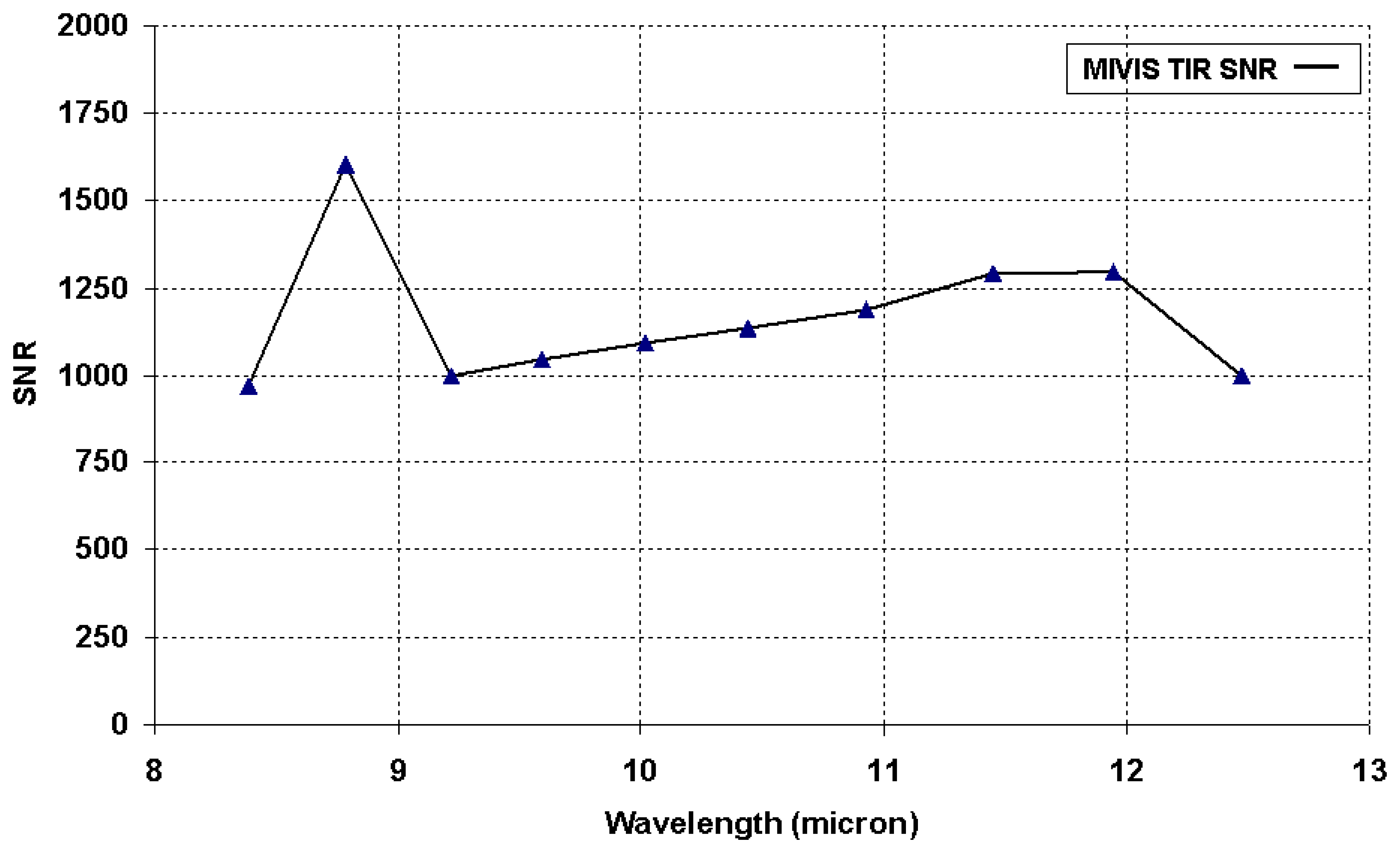
| TIR: 8.18-12.70 μm (channels 93-102) | 340-540 nm | 150 - 1500 | |||
| FOV and IFOV | 71° and 2 mrad | Cross-track pixels | 755 | ||
| Angular | 1.64 | Digitalization accuracy | 12 bit |
©2008 by MDPI Reproduction is permitted for noncommercial purposes.
Share and Cite
Pascucci, S.; Bassani, C.; Palombo, A.; Poscolieri, M.; Cavalli, R. Road Asphalt Pavements Analyzed by Airborne Thermal Remote Sensing: Preliminary Results of the Venice Highway. Sensors 2008, 8, 1278-1296. https://doi.org/10.3390/s8021278
Pascucci S, Bassani C, Palombo A, Poscolieri M, Cavalli R. Road Asphalt Pavements Analyzed by Airborne Thermal Remote Sensing: Preliminary Results of the Venice Highway. Sensors. 2008; 8(2):1278-1296. https://doi.org/10.3390/s8021278
Chicago/Turabian StylePascucci, Simone, Cristiana Bassani, Angelo Palombo, Maurizio Poscolieri, and Rosa Cavalli. 2008. "Road Asphalt Pavements Analyzed by Airborne Thermal Remote Sensing: Preliminary Results of the Venice Highway" Sensors 8, no. 2: 1278-1296. https://doi.org/10.3390/s8021278
APA StylePascucci, S., Bassani, C., Palombo, A., Poscolieri, M., & Cavalli, R. (2008). Road Asphalt Pavements Analyzed by Airborne Thermal Remote Sensing: Preliminary Results of the Venice Highway. Sensors, 8(2), 1278-1296. https://doi.org/10.3390/s8021278