Alpine Grassland Phenology as Seen in AVHRR, VEGETATION, and MODIS NDVI Time Series - a Comparison with In Situ Measurements

Abstract

This study evaluates the ability to track grassland growth phenology in the Swiss Alps with NOAA-16 Advanced Very High Resolution Radiometer (AVHRR) Normalized Difference Vegetation Index (NDVI) time series. Three growth parameters from 15 alpine and subalpine grassland sites were investigated between 2001 and 2005: Melt-Out (MO), Start Of Growth (SOG), and End Of Growth (EOG). We tried to estimate these phenological dates from yearly NDVI time series by identifying dates, where certain fractions (thresholds) of the maximum annual NDVI amplitude were crossed for the first time. For this purpose, the NDVI time series were smoothed using two commonly used approaches (Fourier adjustment or alternatively Savitzky-Golay filtering). Moreover, AVHRR NDVI time series were compared against data from the newer generation sensors SPOT VEGETATION and TERRA MODIS. All remote sensing NDVI time series were highly correlated with single point ground measurements and therefore accurately represented growth dynamics of alpine grassland. The newer generation sensors VGT and MODIS performed better than AVHRR, however, differences were minor. Thresholds for the determination of MO, SOG, and EOG were similar across sensors and smoothing methods, which demonstrated the robustness of the results. For our purpose, the Fourier adjustment algorithm created better NDVI time series than the Savitzky-Golay filter, since latter appeared to be more sensitive to noisy NDVI time series. Findings show that the application of various thresholds to NDVI time series allows the observation of the temporal progression of vegetation growth at the selected sites with high consistency. Hence, we believe that our study helps to better understand large-scale vegetation growth dynamics above the tree line in the European Alps.

1. Introduction

1.1. Scientific Context

The effects of climate variability on ecosystems have in recent decades become increasingly important within the global climate change discussion [1]: earlier start of spring and extended autumn conditions are reflected in phenological time series and result in prolonged growing seasons. This has already been demonstrated in phenological ground observations (e.g. [2–4]) as well as in remote sensing vegetation index time series [5, 6]. Ground observations in combination with remote sensing approaches can make important contributions to future climate-phenology studies [1]. However, ground validation of remote sensing measurements with coarse resolution implies considerable difficulties. Fisher and Mustard [7] state that the poor relationship between ground- and satellite phenology due to data scale issues is a draw-back of satellite phenology, because the chance of a single point ground observation being representative of an entire area at remote sensing scale (typically ≥ 1 km in remote sensing phenology studies; [8, 9]) is small. Comparative studies of satellite and ground based phenology were performed in order to assess the interrelationship of both approaches (e.g. [7, 10–13]). In order to assure the comparability of remote sensing and ground phenological data sets, Fisher and Mustard [7] suggest that the phenological metric to be investigated should ideally be identifiable from ground and space and it should represent the same phenological event from both perspectives. Additionally, the same authors stress the importance of topography in comparative studies such that small-scale phenological heterogeneity due to highly variable topography may lead to discrepancies between remote sensing and ground observations.

The Normalized Difference Vegetation Index (NDVI) is a commonly used remote sensing vegetation index in climate-phenology studies [5, 6, 8, 9, 14]. The NDVI is calculated from the reflectances in the red and near infrared (NIR) bands of the electromagnetic spectrum and is a measure of the photosynthetic activity within the area covered by a pixel [15, 16]. NDVI time series, however, suffer from numerous limitations: the calculated NDVI is not only a function of vegetation density and type, but it is also influenced by the atmosphere and illumination as well as observation geometry, which results in noisy NDVI time series [17, 18]. In order to extract meaningful information on vegetation dynamics regardless of these distortions, various methods for the elimination of spurious data were developed, such as the Maximum Value Composite (MVC; [17]), Best Index Slope Extraction (BISE; [19]), Fourier adjustment [20], Savitzky-Golay filter [21], asymmetric Gaussian model functions [22], and many more. All methods aim at approaching an upper NDVI envelope, based on the assumption that NDVI values are depressed by any of the above-mentioned effects [17]. Smoothing algorithms yet hold the danger of introducing artifacts and suppressing natural variations in the NDVI time series [7].

1.2. Study Overview

The European Alps are assumed to be particularly sensitive to changes in the climate system [23–25]. Plant species have already been observed to migrate to higher elevations as a consequence of climate change [26, 27]. Stöckli and Vidale [14] found a trend towards longer growing season lengths in the European Alps based on the 20-year Pathfinder NDVI data set [28]. Observed changes in growing season length are likely to have considerable implications for ecosystem services, agriculture and nature conservation. It is therefore particularly pressing to understand and quantify past and future changes in season length in mountain ranges on large spatial scales, e.g. with remote sensing approaches. Phenological networks in Switzerland [4, 29] that could serve as ground validation for remote sensing NDVI time series reach up to 1800 m above sea level. However, for higher elevations the Swiss snow-measuring network IMIS (“Interkantonales Mess- und Informationssystem”) can provide data on vegetation growth [30, 31].

The study presented here focuses on the growth phenology of alpine grassland at 15 IMIS sites between 2001 and 2005 from both satellite and ground perspectives. The IMIS network provides an excellent opportunity to link remote sensing and ground phenological measurements in a highly complex environment such as the Swiss Alps, even though frequent cloud cover as well as pronounced topography make the task difficult. Particularly, we investigated the ability of remote sensing NDVI time series to track three IMIS vegetation parameters with special consideration of the 20-year National Oceanic and Atmospheric Administration (NOAA) Advanced Very High Resolution Radiometer (AVHRR) archive of the Remote Sensing Research Group (RSGB), University of Bern. A cross-comparison was subsequently performed with NDVI time series from two newer generation sensors: Système Pour l'Observation de la Terre (SPOT) VEGETATION (VGT; 1 km spatial resolution) and TERRA Moderate Resolution Imaging Spectroradiometer (MODIS; 500 m and 1 km). NDVI time series from all three sensors were smoothed following two different approaches: a Fourier adjustment algorithm modified from Stöckli and Vidale [14] and the Savitzky-Golay method introduced by Chen et al. [21]. The ability of both algorithms to minimize undesirable noise in the NDVI time series was revised for our purposes.

2. Data and Methods

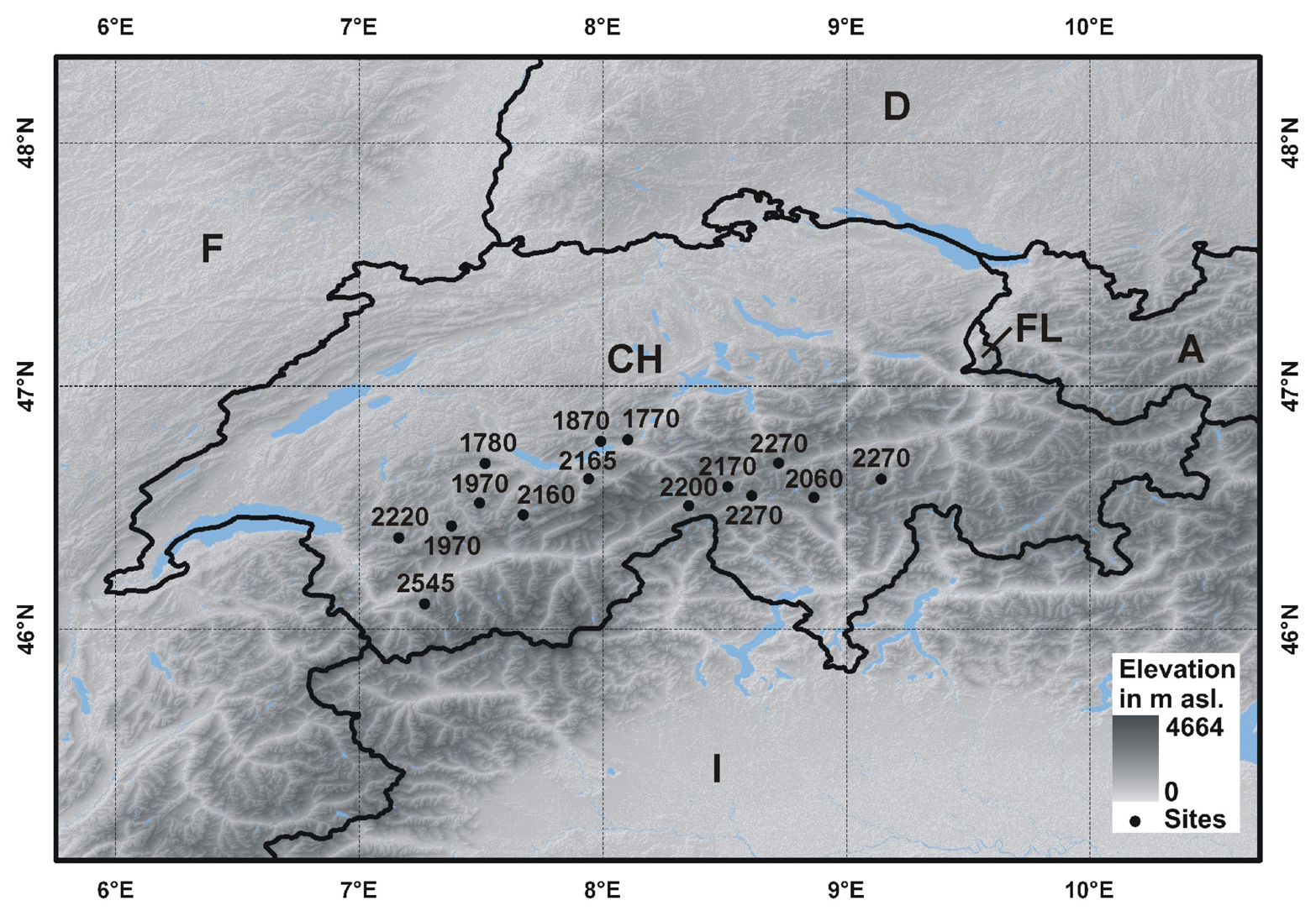
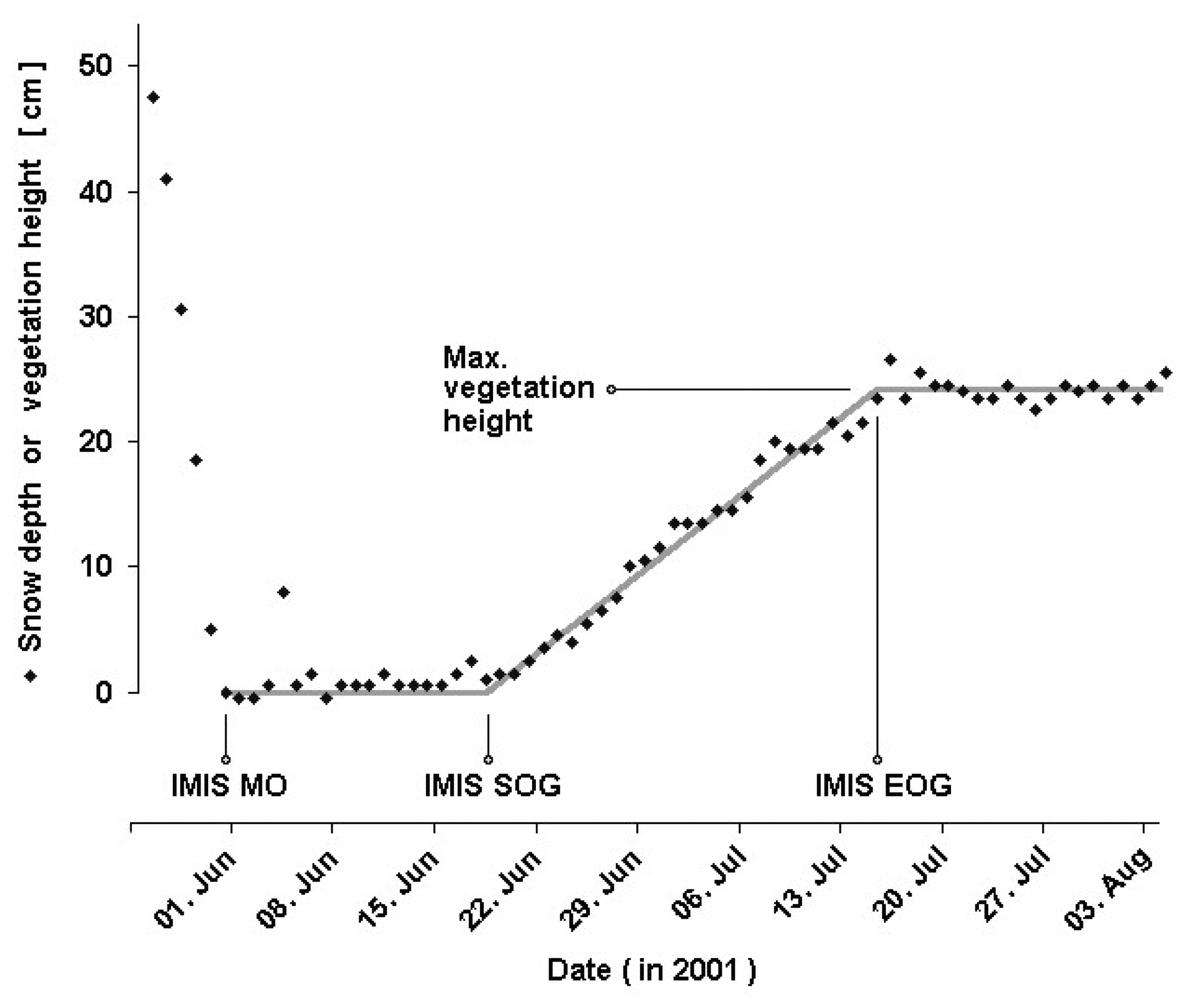
2.1. Ground Data Set

Only a brief overview of the ground data set is provided here. For detailed information we refer to Jonas et al. [31]. The IMIS network is a meteorological network that has been run by the Swiss Federal Institute for Snow and Avalanche Research (SLF) since 1996 [30] and that has since then recorded snow and climate variables such as snow depth, air temperature, wind speed, and soil temperature in 30-minute intervals. More than 100 stations were installed throughout the Swiss Alps. Snow depth is measured from above with an ultrasonic snow depth sensor (mounted on a mast 6 m above ground), which can also track vegetation height during summer. 15 out of 105 stations were identified to best feature undisturbed subalpine and alpine grasslands with a homogeneous vegetation of at least 10 cm height at full growth. The sites are distributed throughout the Swiss Alps and range from 1770 to 2545 m a.s.l. (Figure 1). The combination of meteorological and phenological information at the IMIS sites provides an excellent opportunity to study alpine grassland phenology. IMIS dates or indices were computed by fitting the growth signal with a 3-leg linear fit (bold line, Figure 2): melt-out date (IMIS_MO), which can be regarded as the start of season, start of height growth (IMIS_SOG), and end of growth (IMIS_EOG), which corresponds to the date where maximum plant height is reached. Leaf unfolding after melt-out did typically not result in any detectable height growth until two to three weeks after melt-out, when the onset of vegetation height growth (IMIS_SOG) was observed. IMIS_SOG was followed by a nearly linear growth until maximum vegetation height was reached (IMIS_EOG) in early summer (Figure 2).

A minimum duration of snow cover at the investigated grassland sites spanning from 1 December to 30 April was identified [31]. For the subsequent use within the processing of the remote sensing data, we shortened this snow-covered period by 15 days on either side to define a maximum growing season length at the investigated sites.

2.2. Remote Sensing Data Sets

2.2.1. NOAA AVHRR

The AVHRR data utilized in this study consist of afternoon passes (Equator Crossing Time ≈ 1.30 pm) from the six channel AVHRR/3 instrument on board the polar orbiting NOAA-16 satellite between the 27 February 2001 and 3 October 2005. The nominal instrument spatial resolution at nadir is 1.1 km. Sensor data were calibrated according to the KLM user's guide [32], using the monthly updated coefficients for channels 1 and 2 from the NOAA National Environmental Satellite Data and Information Service (NESDIS). Prelaunch coefficients for channel 1 and 2 calibration were used before these updates started in 2003. A feature matching algorithm was used to achieve sub-pixel accuracy of the geolocation. Orthorectification, which is important to reduce geometric distortions introduced by the complex alpine relief and the scan geometry, was performed using the GTOPO30 digital terrain model. Cloud detection was done using the Cloud and Surface Parameter Retrieval (CASPR) software by Key [33]. The overall quality of the CASPR algorithm was proved by Di Vittorio and Emery [34], however, Hauser et al. [35] who also applied CASPR to NOAA-16 data for a region covering Switzerland observed difficulties arising from sub-pixel clouds. An atmospheric correction in the involved AVHRR channels was not performed. The data were not corrected for NOAA-16 orbital drift, since the effect of solar zenith angle on NDVI is partly compensated for vegetated surfaces [14] and is assumed to be weak, especially in seasonal and inter-annual terms [6].

NDVI time series were subsequently calculated from AVHRR bands 1 and 2 (

Table 1. Spectral characteristics [nm] of the red and NIR bands of all involved sensors, where red=red part of the electromagnetic spectrum and NIR=near infrared part of the spectrum. Red and NIR bands are involved in the calculation of the NDVI.

	AVHRR/3 [32]	VGT [36]	MODIS [37]
red [nm]	580-680	610-680	620-670
NIR [nm]	725-1000	780-890	841-876

). Observations with satellite zenith angles greater than 45° were excluded from further processing in order to avoid large variations in the data due to viewing geometry. Data gaps in early 2001 and late 2005 as pointed out above were dealt with as follows: missing data outside the growing season as outlined in Section 2.1 were set to a value of NDVI=−0.05, since the pixel was assumed to be snow covered at that time of the year. Missing data during the snow free period were set to NDVI=0.0. A Maximum Value Composite (AVHRR_MVC) was subsequently created from the cloud screened daily NDVI data. The MVC technique [17] selects the highest NDVI value within a predefined time interval (i) and is a widely accepted method for the removal of undesirable noise from daily NDVI time series. A value of i=10 days was chosen for the daily AVHRR product.

The drawback of the compositing methodology is the loss of critical temporal information required to accurately track phenological processes. In order to counter this loss, precise acquisition dates for all selected NDVI values were retained instead of assigning constant time steps (i) to the composite NDVI time series.

2.2.2. SPOT VEGETATION

The freely available SPOT VGT-S RADIOMETRY product for Europe (25°N-75°N, −11°E-62°E) was downloaded from the VGT distribution site ( http://free.vgt.vito.be/) for the investigated period (180 scenes totally). The S-10 product represents 10-day composites in 1 km spatial resolution, selecting the pixel with the highest Top of Atmosphere NDVI [36]. NDVI time series at the selected alpine grassland sites were extracted from the NDV band. The precise date of acquisition for each pixel was derived from the time grid (TG) band. Cloud as well as quality flags were extracted from the status map (SM). For more detailed information about the VGT-S10 product we refer to the VEGETATION Programme [36].

All cloudy NDVI values that occurred during the snow covered period were set to a value of −0.05. Values from cloudy days during the growing season were linearly interpolated between the previous and subsequent NDVI value. The same procedure was applied to all points where the quality flag in either the red or the near infrared band (Table 1) revealed less than ideal quality.

2.2.3. TERRA MODIS

The MODIS tile number h18/v4 (40°N-50°N, 0°E-15.6°E) of the MOD09A1 surface reflectance product with a spatial resolution of 500 m was downloaded from the Land Processes Distributed Active Archive Center (LP DAAC; http://edcdaac.usgs.gov/main.asp) for the investigated period (225 scenes in total). The MOD09A1 product represents 8-day composites, selecting observations with minimal cloud cover and favorable observation geometry (low solar and satellite zenith angles). MODIS scenes were resampled to UTM 32N (WGS84) prior to further processing.

NDVI time series were calculated from the surface reflectance in MODIS bands 1 and 2 (Table 1). The precise acquisition date for each pixel is provided along with the MOD09A1 product in an auxiliary data set. Cloud state as well as quality flags were extracted from the surface reflectance state flags. The same interpolation procedure for cloudy and not ideal quality NDVI values was performed as described in Section 2.2.2 along with the preprocessing of the VGT-S data.

In order to assess the impact of spatial NDVI product resolution on the comparison with IMIS ground data, a surface reflectance product with 1 km spatial resolution was generated based on the original 500 m MOD09A1 product using bilinear resampling. Further processing of the 1 km product was performed according to the procedure as described above for the 500 m product. The 1 km NDVI product was finally calculated from the 1 km surface reflectance product, and cloudy as well as not-ideal quality NDVI values were interpolated using the same procedure as for the VGT-S data.

2.3. Application of Smoothing Algorithms

The process of compositing is not sufficient to eliminate all unrealistic variability from NDVI time series [22]. Two widely used smoothing approaches were therefore modified (below described in detail) and applied to the composite NDVI time series (NDVI_comp) in order to test for their capability to minimize undesirable noise in the composite NDVI time series at the selected 15 alpine grassland sites: a Fourier adjustment algorithm modified from Stöckli and Vidale [14] based on Sellers et al. [20], and an adaptive Savitzky-Golay filter as it was introduced by Chen et al. [21]. Smoothing algorithms were applied to isolated single year time series (i.e. from January to December). Only modifications to the above-mentioned algorithms are dealt with in the following sections.

2.3.1. Fourier Adjustment

Unevenly spaced composite NDVI time series (i.e. precise acquisition dates for all NDVI values) as described here for all three sensors do not meet the requirements of the above mentioned Fourier adjustment algorithm, which assumes constant intervals in time. The algorithm was therefore applied to time series with daily, and hence constant, time steps (NDVI₃₆₅). For that purpose composite NDVI time series were complemented with auxiliary NDVI values (NDVI_aux=−1) in between the valid points that had been pre-selected within compositing. In order to get a rough approximation of seasonality in the NDVI time series, a second order Fourier series (f) was fitted to NDVI₃₆₅ using non-linear least squares, assigning weights of W_valid=1 to all valid and W_aux=0 to all auxiliary points. Data were flagged as anomalous if they were outside the boundary (f_comp−2σ) < NDVI_comp < (f_comp+2σ), where f_comp represents the values of f at the corresponding dates of NDVI_comp, and σ is the standard deviation of (f_comp−NDVI_comp). Anomalous NDVI_comp values were subsequently linearly interpolated between the previous and following valid point. Screened NDVI_comp were again transformed into a time series with daily time steps for further processing, assigning NDVI_aux to the missing dates.

In the following we fitted third order Fourier series, since it turned out that the very pronounced NDVI increase in spring and decrease in late fall at the selected sites could not be represented in second order series (not shown). The weighting scheme [14], which assigns higher weights to uncontaminated measurements than to negative outliers, was only applied during the growing season. Here again, W_aux=0 were assigned to all NDVI_aux of the daily resolution time series. The high temporal resolution (1 day) of the resulting Fourier adjusted NDVI time series can be advantageous when comparing satellite and ground based phenological events. An example of a Fourier adjusted NDVI time series is displayed in Figure 3 for the Dötra site, 2060 m a.s.l.

2.3.2. Savitzky-Golay Filter

The Savitzky-Golay filter [38] performs a local polynomial least squares fit within a moving window to assign a smoothed value to each underlying data point. In contrast to simple moving average filters, this filter preserves area, mean position, width, and height of seasonal peaks in NDVI time series [39]. Like the Fourier adjustment algorithm, the Savitzky-Golay filter requires NDVI data with uniform temporal intervals, however, the use of NDVI time series with daily resolution (taking into account precise acquisition dates as demonstrated for the Fourier algorithm) did not reveal satisfactory results (not shown). Hence, dates corresponding to the MVC time interval center (i/2) were assigned to each NDVI value in order to create an evenly spaced composite NDVI time series (NDVI_even) with a temporal resolution of i=10 days. All values outside the boundary (f−2σ) < NDVI_even < (f+2σ) were flagged as anomalous, where f is a second order Fourier series that was fitted to NDVI_even and σ the standard deviation of (f−NDVI_even). Anomalous NDVI_even values were subsequently linearly interpolated between the previous and following valid point and steps 2 to 7 of the suggested procedure in Chen et al. [21] were applied to screened NDVI_even. Once the NDVI time series was filtered, a curve was fitted to the data points using linear interpolation to obtain daily resolution. An example of a Savitzky-Golay adapted NDVI time series is displayed in Figure 3.

2.4. Comparison of Remote Sensing and Ground Data

The ability of remote sensing NDVI time series to track the IMIS vegetation growth dates IMIS_MO, IMIS_SOG, and IMIS_EOG was tested using the threshold method. A threshold (th) represents a certain fraction of the maximum annual NDVI range (NDVI_MAX − NDVI_MIN; Figure 3). The date where the threshold is crossed for the first time designates the vegetation growth parameter in the NDVI time series (analogous to IMIS dates: NDVI_MO, NDVI_SOG, and NDVI_EOG). Keeping in mind that the NDVI is a measure of photosynthetic activity and therefore can be related to aboveground biomass [40], we expect leaf unfolding after melt-out as well as grassland height growth to be represented in the NDVI time series as various NDVI levels, i.e. at a certain percentage of the maximum annual greenness of each pixel. The threshold method, however, strongly depends on single data points (NDVI_MAX and NDVI_MIN) and is hence sensitive to errors in the timing and magnitude of both NDVI bounding values [12].

The relationship between remote sensing and ground data sets was on the one hand quantified by calculating the linear correlation coefficient (r) of remote sensing and ground growth phenological dates, and on the other hand by the determination of the mean temporal offset in days $(\overline{OD})$between the two data sets, with OD representing the temporal offsets in days between remote sensing and ground data sets for each phenological date, site and year. Several thresholds were tested for each pixel and phenological date in order to identify which thresholds yielded lowest $\overline{OD}$. The mean offset in days $\overline{OD}$adopted negative values where the growth parameter was estimated too early in the year by the remote sensing NDVI data set, i.e. where th was chosen too low. Analogously, $\overline{OD}$ adopted positive values where th was chosen too high. Figure 4 addresses this issue, showing an example of a relationship between satellite and ground data where th was chosen too low (left), nearly optimal (middle) and too high (right). In the first case the majority of the points are below the 1:1 line, gradually shifting upwards with increasing thresholds (middle and right). OD for each point is given by its vertical distance from the 1:1 line. The scatter as seen in the subplots of Figure 4 was therefore described as the OD standard deviation (σ in Figure 4 and

Table 2. Relationship between phenological growth dates of alpine grassland from four remote sensing NDVI time series ([a-d]; each smoothed with two smoothing algorithms) and IMIS sensor ground data, where MO=melt-out, SOG=start of growth, EOG=end of growth, th=applied threshold, r=linear correlation coefficient of satellite and ground data set, and $\overline{OD}=$mean temporal offset in days between satellite and ground data set ± one standard deviation (σ). Several thresholds were tested for each parameter, NDVI product, and sensor. Shaded thresholds indicate lowest $\overline{OD}$ with regard to the other thresholds. All correlations were significant with p < 0.001 (two-tailed).

	[a] AVHRR (1 km)				[b] VEGETATION (1 km)				[c] MODIS (500 m)				[d] MODIS (1 km)
Fourier
N=55	th	r	$\overline{OD}$		th	r	$\overline{OD}$		th	r	$\overline{OD}$		th	r	$\overline{OD}$
MO	0.5	0.61	−7.1±13.3	MO	0.5	0.78	−3.6±11.0	MO	0.4	0.82	−7.3±9.8	MO	0.4	0.8	−6.8±11.4
	0.6	0.61	0.3±13.4		0.6	0.78*	3.5±10.9		0.5	0.82*	−0.5±9.9*		0.5	0.8*	0.2±11.7
	0.7	0.60	7.9±13.4		0.7	0.79	10.7±10.8		0.6	0.82	6.3±9.9		0.6	0.81	7.1±11.3
SOG	0.7	0.63	−6.2±13.4	SOG	0.7	0.77	−3.4±11.4	SOG	0.6	0.79	−7.8±10.8	SOG	0.6	0.75	−7.0±12.6
	0.75	0.64	−2.2±13.3		0.75	0.77	0.5±11.3		0.7	0.79	−0.6±10.7		0.7	0.75	0.4±12.4
	0.8	0.64	2.2±13.2		0.8	0.77	4.7±11.3		0.75	0.79	3.3±10.8		0.75	0.75	4.3±12.3
EOG	0.95	0.67	−6.4±12.8	EOG	0.95	0.72	−3.4±12.9	EOG	0.9	0.77	−8.7±11.7	EOG	0.9	0.75	−8.0±12.4
	0.98	0.68	0.7±12.4••		0.98	0.69	3.2±13.2		0.95	0.76	−1.5±12.4••		0.95	0.74	−1.0±12.4
	1.0	0.66	12.7±12.6		1.0	0.67	14.4±13.5		0.98	0.74	4.7±12.9		0.98	0.74	5.4±12.4
Savitzky-Golay
N=55	th	r	$\overline{OD}$		th	r	$\overline{OD}$		th	r	$\overline{OD}$		th	r	$\overline{OD}$
MO	0.5	0.55	−5.3±14.4	MO	0.5	0.76	−7.9±11.2	MO	0.4	0.79	−4.8±11.9	MO	0.4	0.81	−4.7±11.6
	0.6	0.53	1.5±15.0		0.6	0.76*	−2.4±11.2*		0.5	0.81**	0.3±11.3*		0.5	0.81**	0.6±11.4
	0.7	0.52	7.8±15.5		0.7	0.76	3.6±11.3		0.6	0.80	4.6±11.5		0.6	0.8	5.6±11.8
SOG	0.7	0.59	−6.4±14.7	SOG	0.75	0.76	−7.1±11.4	SOG	0.7	0.79	−3.8±11.4	SOG	0.7	0.75	−3.4±13.0
	0.75	0.57	−1.6±14.7		0.8	0.76*	−3.5±11.5		0.75	0.79*	−0.5±12.4		0.75	0.73	−0.1±13.6
	0.8	0.47	3.0±17.3		0.9	0.72	6.9±12.4		0.8	0.78	3.4±13.2		0.8	0.74	3.1±13.8
EOG	0.9	0.50	−13.0±18.5	EOG	0.95	0.71	−11.4±13.1	EOG	0.95	0.63	−4.8±17.4	EOG	0.95	0.74	−9.1±13.6
	0.95	0.51	−3.7±20.1		0.98	0.64	−2.5±15.2*		0.98	0.63	0.7±17.7		0.98	0.72*	−1.7±14.5*
	0.98	0.60	5.2±18.2		1.0	0.49	8.5±19.5		1.0	0.57	11.8±19.8		1.0	0.63	8.9±18.0

Significant differences between equivalent values of r and σ, respectively, (for shaded thresholds only) are indicated for i) the comparison of AVHRR with the newer generation sensors (horizontal, **:1%-level, *:5%-level, one-tailed) and ii) the comparison between smoothing algorithms (vertical, ^••:1%-level, two-tailed). Comparisons within the MODIS products (500 m and 1 km) did not reveal significant differences.

) in addition to the linear correlation coefficient r. These analyses were carried out for eight NDVI data sets from all 4 products (AVHRR, VGT, MODIS 500 m, and MODIS 1 km), each smoothed with both filter methods (i.e. Fourier adjustment and Savitzky-Golay filter; Table 2). Differences in correlation coefficients were tested performing the Fisher r-to-z transformation, standard deviations of the offset in days by means of the F-test. In the following, p-values of p < 0.01 were termed as highly statistically significant and p < 0.05 as statistically significant.

3. Results

Out of the three thresholds that were tested for each phenological event, smoothing algorithm, and sensor, shaded thresholds in Table 2 generally represent the lowest mean offset in days $(\overline{OD})$. For the same phenological date, the best thresholds (i.e. yielding min. $\overline{OD}$) were very similar across all sensors and smoothing methods. On the other hand, the optimum thresholds for different phenological dates showed clear differences. All best (shaded) threshold values ranged between 0.5 and 0.6 for MO, between 0.7 and 0.75 for SOG and between 0.95 and 0.98 for EOG. Hence, an effect of spatial NDVI product resolution on the determination of the thresholds was not found for the MODIS 500 m and 1 km products, i.e. best thresholds (Table 2 [d]) remained unchanged with reduced spatial resolution.

Correlations were highly significant across all data sets and smoothing algorithms, with linear correlation coefficients adopting values between r=0.51 and r=0.82 (Table 2). Overall best correlations were obtained by the Fourier adjusted MODIS 500 m NDVI data set. Overall lowest correlations were obtained for EOG extraction by means of the Savitzky-Golay filtered NDVI time series. In general, large standard deviations of OD were observed (cp. Table 2), with highest standard deviations obtained for the AVHRR product and lowest standard deviations obtained for the MODIS 500 m product (Figure 4).

3.1. Comparison of AVHRR NDVI Time Series and IMIS phenological dates

Differences in smoothing algorithm performance were apparent (significance levels indicated in Table 2): the Fourier adjusted NDVI data exhibited overall higher correlations with the IMIS phenological dates than the Savitzky-Golay filtered data, however, this difference was not statistically significant. Additionally, OD standard deviation was generally found to be higher for the Savitzky-Golay filtered data set compared to the Fourier adjusted data, with the difference in OD standard deviation for the detection of EOG being highly significant. No obvious pattern was found in terms of which phenological event showed highest correlations within one respective data set: within the Fourier adjusted AVHRR NDVI time series, EOG displayed highest correlations (MO lowest), whereas within the Savitzky-Golay filtered data, SOG exhibited highest correlations (EOG lowest).

3.2. Comparison to VGT and MODIS products

Differences in smoothing algorithm performance were not as pronounced for the investigated newer generation sensors compared to AVHRR, even though Fourier adjusted NDVI time series generally exhibited slightly higher correlations compared to the Savitzky-Golay filtered time series. OD standard deviations were highly significantly different for EOG detection using the MODIS 500 m product (significance levels indicated in Table 2).

All VGT as well as MODIS NDVI products exhibited higher correlations compared to AVHRR, but the difference was not statistically significant in all investigated cases (Table 2 [b-d]): Differences within the Fourier adjusted data sets were e.g. significant for the detection of MO, but not significant for EOG detection. Correlations of IMIS phenological dates and 1 km MODIS NDVI time series were not significantly lower compared to the MODIS 500 m product and were comparable to the correlations as obtained for the VGT NDVI product (also 1 km).

OD standard deviations of all newer generation products were lower compared to AVHRR. Differences in OD standard deviations were e.g. statistically significant for EOG detection by means of the VGT and MODIS 1 km Savitzky-Golay filtered data sets compared to AVHRR. An minor effect of spatial resolution was detected in terms of OD standard deviation, which was found to increase with lowered spatial resolution. This effect was more pronounced for the Fourier adjusted NDVI data compared to the Savitzky-Golay filtered data. OD standard deviations of the Fourier adjusted 1 km MODIS product appeared to be of the same order of magnitude as the standard deviations obtained with the 1 km VGT data sets, but lower compared to the AVHRR NDVI data.

4. Discussion

The good agreement between the spectral remote sensing measurements and the single point vegetation height measurements in highly complex terrain was remarkable, especially in consideration of the large differences in measurement scales. Robustness of the results was reflected in consistent thresholds among all NDVI products and phenological events and is encouraging with regard to further phenological studies within complex alpine environments.

Numerous previous studies have investigated the relationship between remote sensing and ground measured vegetation indices as well as biophysical parameters in a wide range of grassland ecosystems [13, 40–43], including such in the European Alps [44, 45]. By contrast to these studies, our study focused on the resolution of annual growth dynamics of alpine grassland. We believe that relating threshold derived phenological dates from remote sensing NDVI time series to ground phenological data from the IMIS network was an important step towards a better understanding of broad scale vegetation growth dynamics above the tree line in the European Alps.

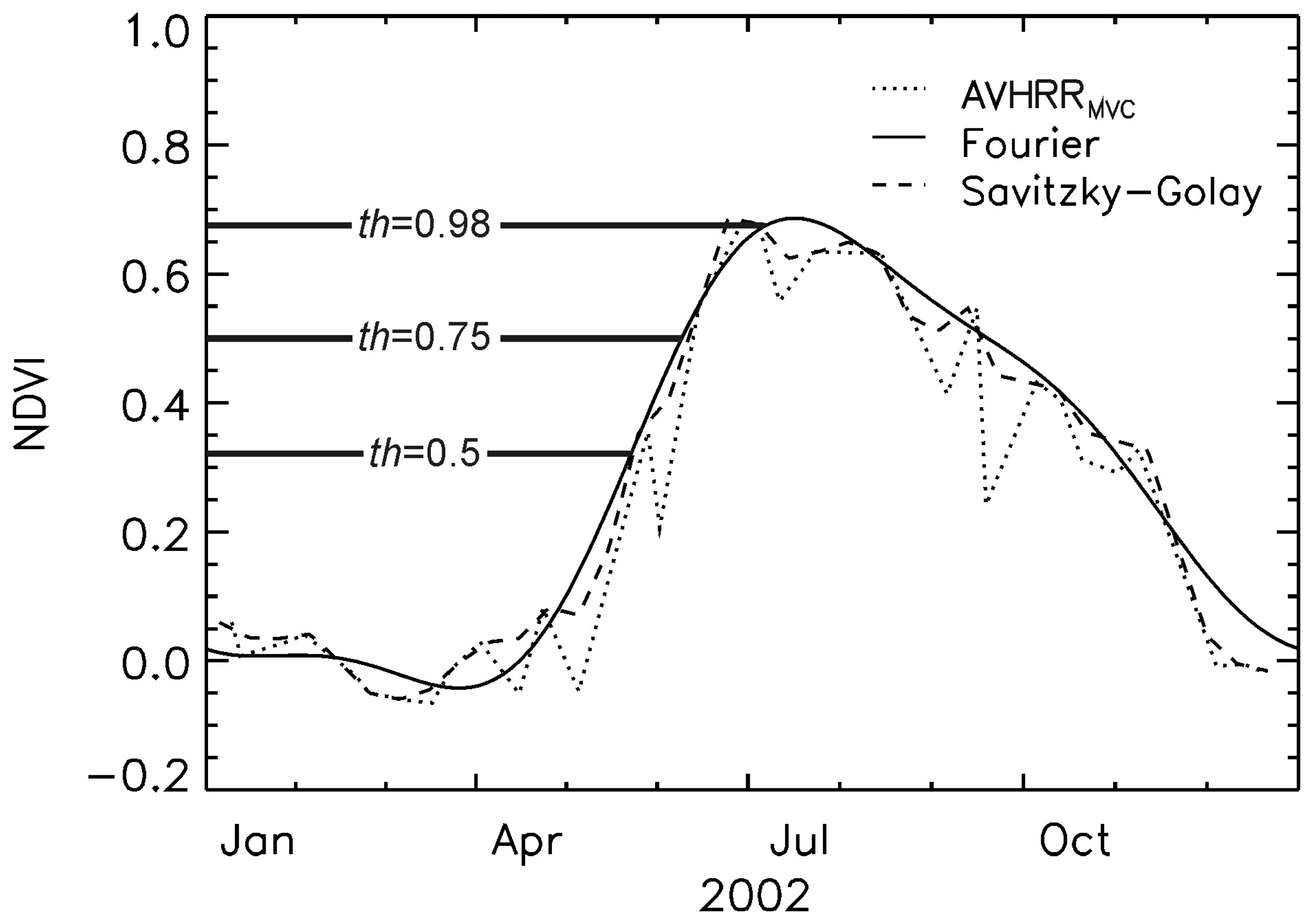
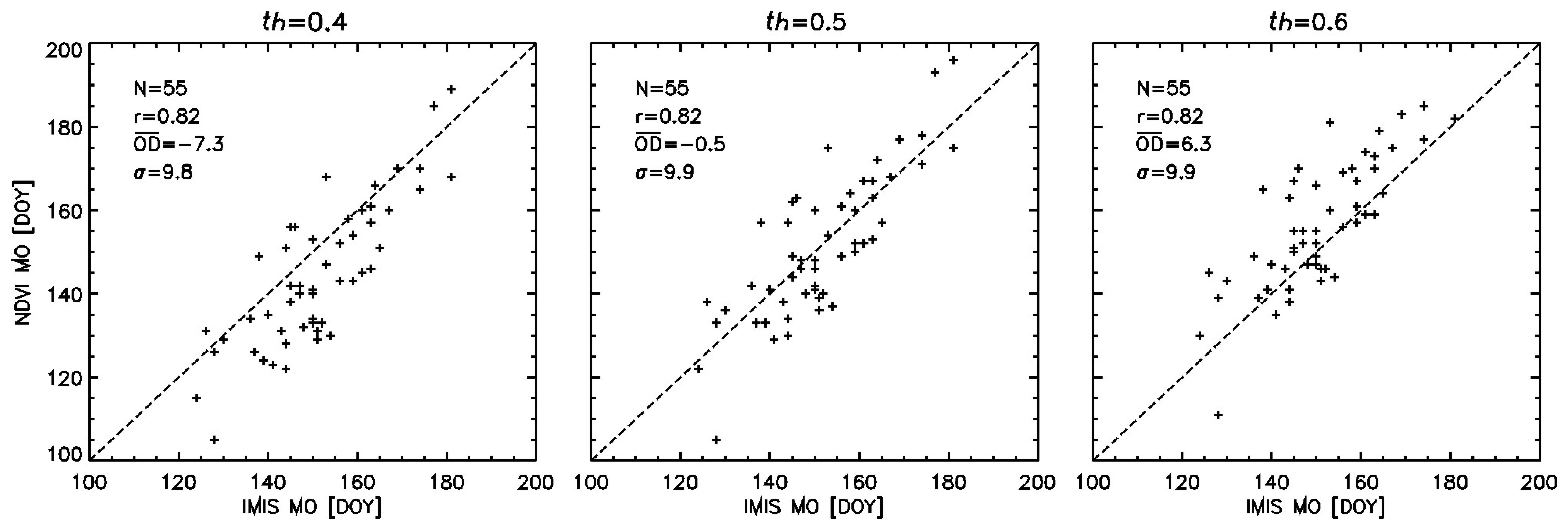
4.1. Determination of Thresholds

Optimal thresholds were only investigated with a precision of 0.1 (MO), 0.05 (SOG), and 0.02/0.03 (EOG). A larger data set would be needed in order to determine precise thresholds for each NDVI data set and parameter. However, the good agreement between both satellite and ground data sets still enables us to identify following approximate thresholds to be suitable to determine grassland growth phenology with NDVI time series at the selected 15 IMIS sites:

• Melt-out: th≈0.6
• Start of growth: th≈0.75
• End of growth: th≈0.98

Even though year-to-year melt-out variability at the selected sites is very high (below described in detail), melt-out dates from ground and remote sensing data sets showed a good agreement. Independent of sensor and smoothing algorithm, thresholds of approx. th=0.6 seemed to be appropriate to track MO, which can be regarded as the start of season. This threshold for the determination of the start of season is slightly higher compared to the threshold as it was applied e.g. in Stöckli and Vidale [14] to a NDVI data set with 0.1° spatial resolution. Stöckli and Vidale [14] applied a threshold of th=0.4 to the entire Alps subdomain in order to derive start of season dates for a period of 20 years. However, lower spatial resolution of the latter NDVI product renders a comparison of both thresholds difficult, since first of all, the variability of the occurrence of phenological events within a pixel will increase with lower spatial resolution, and second, an area of 0.1° × 0.1° within the European Alps will most likely include land cover classes other than grassland. It will therefore exhibit different annual NDVI dynamics compared to the higher resolution NDVI data sets as used in this study. This issue emphasizes the necessity of adapting thresholds to specific land cover classes. Based on these considerations, we suggest that whether or not the presented thresholds are applicable to coarser resolution NDVI products critically depends on the homogeneity of land cover and terrain within the investigated area.

SOG dates, which at the ground usually were observed two to three weeks after MO, coincided with the date where approximately 75% of the total annual NDVI amplitude were crossed, corresponding to th=0.75. The differences in the threshold magnitude between MO and SOG reflect the increased pixel integrated greenness due to leaf unfolding and build up of leaf biomass after snow melt. Then again, EOG dates were generally identified in remote sensing data shortly before NDVI time series reached saturation (NDVI_MAX). The fact that IMIS_EOG nearly coincided with NDVI_MAX is a highly interesting finding, suggesting that maximum photosynthetic activity of alpine grassland is achieved at the end of height growth, i.e. when vegetation has reached its maximum height.

Since the decrease of spatial resolution from 500 m to 1 km did not have an effect on the determination of the thresholds, we suggest that thresholds for alpine grassland to a major extent depend on the spectral characteristics of the sensor: according to Table 1 red bands of the considered sensors all encompass different parts of the spectrum in the red domain, hence being variably sensitive to changes in chlorophyll concentration within the grassland pixel [46]. Positions of the channels in the visible domain of the electromagnetic spectrum can thereby influence the magnitude of the NDVI [47] and the shape of the NDVI curve. Thus, differences in spectral band widths and locations (Table 1) lead to variable NDVI dynamic ranges (NDVI_MAX−NDVI_MIN) among the sensors [13] as well as to different timings of NDVI_MAX, i.e. NDVI saturation. The determination of the thresholds is thereby influenced. The time of occurrence of NDVI_MAX is particularly important for the extraction of EOG from remote sensing NDVI time series, since the thresholds were found to be close to th=1.0, i.e. close to NDVI_MAX itself. The magnitude of the NDVI as well as the shape of the NDVI curve also depend on the reduction of the atmospheric influence in both channels, since NDVI values are depressed by atmospheric influence [18]. This issue is discussed in more detail below.

The shape of the NDVI curve is to a certain extent also influenced by the nonuniform distribution of bidirectional reflectance (BRD), which results in surface reflectance – and hence NDVI – variations depending on the observation geometry (relative positions sun–target–sensor; [48, 49]). However, it was also shown that BRD effects are significantly reduced through the calculation of vegetation indices such as the NDVI from single channel data [17, 50] and minimized through the process of compositing [17].

4.2. Smoothing Algorithm Performance

Even though the differences in r and σ between the two smoothing approaches were mostly statistically insignificant, results as summarized in Table 2 suggest that for our purposes the Fourier algorithm was more efficient in eliminating undesirable noise from the NDVI time series. Since Savitzky-Golay NDVI products closely follow the composite NDVI times series (Figure 3), they are more sensitive to short term NDVI variations and therefore more susceptible to noisy data. This is most clearly reflected in EOG detection by means of the Savitzky-Golay filtered NDVI time series, where linear correlation coefficients were lowest and OD standard deviation values highest among all investigated cases: noisy time series during the growing season led to multiple local NDVI maxima. Since thresholds for the determination of EOG were found to be close to th=1.0 (i.e. NDVI_MAX), the chance that EOG was attributed to the wrong NDVI peak was high. This issue underlines a drawback of the threshold methodology (Section 2.4), i.e. that the determination of phenological dates from NDVI time series using a fraction of the maximum annual NDVI amplitude may be influenced by errors in the magnitude and timing of both bounding values. Third order Fourier series on the other hand can only track changes in vegetation with a periodicity of 4 months and are therefore less susceptible to noisy composite time series. Residual noise in the Fourier adjusted NDVI time series could be avoided by choosing lower order Fourier series, however, we argue that third order Fourier series represent a good trade-off between noise removal on the one hand and representation of natural NDVI short term variations on the other hand.

As mentioned in Section 2.2.1 the process of compositing comes along with a loss of temporal information. The application of the Fourier algorithm to NDVI time series with daily time steps (considering precise acquisition dates) certainly helped to overcome this issue to a certain extent. By contrast, the temporal uncertainty introduced to the Savitzky-Golay filtered data sets by assigning fixed time intervals of i=10 (Figure 3) likely added to the lower performance of the Savitzky-Golay filtered NDVI data sets.

4.3. AVHRR vs. Newer Generation Sensors

The fact that all three sensors turned out to be capable of tracking alpine grassland dynamics at the selected sites is encouraging with regard to the analysis of the 20-year AVHRR archive. However, results as summarized in Table 2 revealed drawbacks of AVHRR compared to the newer generation sensors (though not statistically significant in all cases). Differences in spectral sensor characteristics likely added to this effect (Table 1). This is particulary important regarding the NIR band, where clear differences between AVHRR and the newer generation sensors are apparent. The AVHRR NIR band is superimposed on strong water vapor absorption bands between 900-980 nm, whereas VGT and MODIS NIR bands do not cover these absorption bands and are hence less affected by variations in atmospheric water vapor content [51, 52]. This effect is enhanced by the fact that both VGT and MODIS data include atmospheric correction, whereas AVHRR data were not corrected for these effects. Even though VGT and MODIS data both include atmospheric correction, Fensholt et al. [13] found discrepancies between VGT and MODIS in the reflectance values of the NIR bands due to differences in atmospheric correction schemes.

Noisy composite NDVI time series were in some cases still observed for all three sensors even after quality and cloud screening, even though unrealistic NDVI values ideally are discarded through the process of compositing. In general, remaining noise in the NDVI time series could be attributed to – for remote sensing applications – hindering weather conditions in terms of extended cloudy periods during the growing season. While in the Alps less cloud cover is observed in winter (December through February) compared to the foreland, the opposite applies to the summer months (June through August), when frequent cloud cover is observed due to orographically induced convection [53, 54]. In the case of AVHRR, insufficient cloud masking by the CASPR algorithm as outlined above likely added to the observed noise in the time series and thereby contributed to the lower performance of AVHRR.

4.4. Explanation of OD Standard Deviation

Complex alpine and subalpine topography leads to high snow cover variability in space and time due to terrain effects on various climatic variables such as wind, precipitation, and snow fall [55, 56]. The resulting “patchy mosaic” [57] of vegetation and snow cover during the period of snow melt results in high year to year NDVI variability within the area around each IMIS site, regardless of the snow and vegetation conditions at the site itself. This random effect adds to the between-year variability of observed phenological dates such that a pixel in one year may exhibit a vegetation signal before, and in another year after it is observed at the IMIS site. Land cover is another crucial factor, which has to be taken into account in this respect due to the limited spatial extent of the investigated grassland areas of sometimes only a few square kilometers: depending on varying pixel size due to observation geometry contaminating land cover classes other than grassland might have influenced the shape of the annual NDVI curve and hence the extraction of phenological dates in some cases.

Even though the locations of the IMIS sites were chosen to be representative of the direct site environment [30], systematic offsets between remote sensing and ground data may be expected according to the location of the IMIS site within its surrounding topography: phenological dates from elevated sites (IMIS site above median elevation of pixel) will presumably be estimated too early by the NDVI, since the phenology at such IMIS sites lags behind the average phenology of the (lower) surroundings. The opposite effect is expected for valley sites (IMIS site below median elevation of pixel). Similar small-scale effects of topography have already been stressed by Fisher et al. [12]. Given the limited number of 15 sites, here this issue cannot be addressed in more detail. However, another data set consisting of five years of melt-out dates from another 69 sites throughout the Swiss Alps will be available for that purpose in the near future.

Interestingly, OD standard deviations of the 1 km MODIS Fourier and VGT data sets were of comparable magnitude, leading to the assumption that OD standard deviation also depends on spatial sensor resolution. That again is in good agreement with the above mentioned issue of small-scale vegetation and snow cover variability [57] as well as the influences of multiple land cover classes in the surroundings of the site: both effects obviously become less pronounced with enhanced spatial resolution.

5. Conclusion and Outlook

The capability of NOAA AVHRR NDVI time series to track alpine grassland phenology was investigated with regard to the analysis of our 20 year AVHRR archive. Three grassland growth phenological dates (melt-out, start of growth, and end of growth) were extracted from NDVI time series and compared to equivalent measurements from the IMIS network at 15 sites in the Swiss Alps. The same investigations were performed for three additional NDVI products from newer generation sensors VGT and MODIS.

The good agreement between single point vegetation height and coarse scale remote sensing measurements was remarkable. Even though correlations were lower for AVHRR compared to the newer generation sensors, results for AVHRR were encouraging with regard to long-term vegetation dynamics analysis in the Swiss Alps. The ability of the tested Fourier adjustment algorithm to minimize undesirable noise from the NDVI time series at the selected sites must be rated higher compared to the Savitzky-Golay product, since the Fourier product is less susceptible to noisy composite time series. Similar thresholds for the determination of grassland phenological dates across sensors and smoothed NDVI products demonstrated the high robustness of the results. Findings for all three sensors show that the application of various thresholds to NDVI time series allows the observation of the temporal progression of vegetation growth at the selected sites with high consistency. Minor threshold differences among the investigated NDVI products are assumed to result from variable spectral sensor characteristics in the red bands, which govern chlorophyll sensitivity, and thereby influence the annual NDVI range.

Discrepancies between remote sensing and ground data sets are assumed to result from small-scale phenological variability due to complex topography as well as from land cover classes other than grassland in the surroundings of the sites. These assumptions are supported by the fact that discrepancies are smaller for the 500 m spatial resolution MODIS product compared to the equivalent 1 km product. Overall, ground based data from the IMIS station network provided a valuable tool to better understand and interpret remote sensing NDVI data.

Investigations will be extended to a larger number of sites and years as soon as the particular data will be available. In order to assess the reasons for the discrepancies between remote sensing and ground data, the incorporation of topographic information in data analysis will be necessary. The inclusion of additional ground verification sites in combination with topographic information will significantly improve our understanding of the relationship between remote sensing and ground phenological measurements in a complex environment such as the Swiss Alps. Additionally, AVHRR data from other NOAA satellites will be included in order to assess the transferability of the results to other satellites of the NOAA series. This will finally enable us to investigate changes in alpine vegetation dynamics on a larger spatial scale for the past 20 years with high spatial and temporal resolution based on the RSGB AVHRR archive. Knowledge about these changes will significantly enhance our understanding of the potential future impact of climate warming on sensitive alpine ecosystems.

References

1. Studer, S.; Stöckli, R.; Appenzeller, C.; Vidale, P. A comparative study of satellite and ground-based phenology. International Journal of Biometeorology 2007, 51, 405–414. [Google Scholar]
2. Menzel, A. Trends in phenological phases in Europe between 1951 and 1996. International Journal of Biometeorology 2000, 44, 76–81. [Google Scholar]
3. Roetzer, T.; Wittenzeller, M.; Haeckel, H.; Nekovar, J. Phenology in central Europe - differences and trends of spring phenophases in urban and rural areas. International Journal of Biometeorology 2000, 44, 60–66. [Google Scholar]
4. Defila, C.; Clot, B. Phytophenological trends in Switzerland. International Journal of Biometeorology 2001, 45, 203–207. [Google Scholar]
5. Myneni, R.B.; Keeling, C.D.; Tucker, C.J.; Asrar, G.; Nemani, R.R. Increased plant growth in the northern high latitudes from 1981 to 1991. Nature 1997, 386, 698–702. [Google Scholar]
6. Zhou, L.; Tucker, C.J.; Kaufmann, R.K.; Slayback, D.; Shabanov, N.V.; Myneni, R.B. Variations in northern vegetation activity inferred from satellite data of vegetation index during 1981 to 1999. Journal of Geophysical Research 2001, 106, 20069–20084. [Google Scholar]
7. Fisher, J.I.; Mustard, J. F. Cross-scalar satellite phenology from ground, Landsat, and MODIS data. Remote Sensing of Environment 2007, 109, 261–273. [Google Scholar]
8. White, M.A.; Thornton, P.E.; Running, S.W. A continental phenology model for monitoring vegetation responses to interannual climatic variability. Global Biogeochemical Cycles 1997, 11, 217–234. [Google Scholar]
9. Reed, B.C.; Brown, J.F.; VanderZee, D.; Loveland, T.R.; Merchant, J.W.; Ohlen, D.O. Measuring phenological variability from satellite imagery. Journal of Vegetation Science 1994, 5, 703–714. [Google Scholar]
10. Chen, X.; Xu, C.; Tan, Z. An analysis of relationships among plant community phenology and seasonal metrics of Normalized Difference Vegetation Index in the northern part of the monsoon region of China. International Journal of Biometeorology 2001, 45, 170–177. [Google Scholar]
11. Braun, P.; Hense, A. Combining ground-based and satellite data for calibrating vegetation indices. Proceedings SPOT 4/5 Vegetation unser's Conference, Antwerp; 2004; pp. 137–141. [Google Scholar]
12. Fisher, J.I.; Mustard, J.F.; Vadeboncoeur, M.A. Green leaf phenology at landsat resolution: Scaling from the field to the satellite. Remote Sensing of Environment 2006, 100, 265–279. [Google Scholar]
13. Fensholt, R.; Sandholt, I.; Stisen, S. Evaluating MODIS, MERIS, and VEGETATION vegetation indices using in situ measurements in a semiarid environment. IEEE Transactions on Geoscience and Remote Sensing 2006, 44, 1774–1786. [Google Scholar]
14. Stöckli, R.; Vidale, P.L. European plant phenology and climate as seen in a 20 year AVHRR land-surface parameter dataset. International Journal of Remote Sensing 2004, 25, 3303–3330. [Google Scholar]
15. Justice, C.O.; Townshend, J.R.G.; Holben, B.N.; Tucker, C.J. Analysis of the phenology of global vegetation using meteorological satellite data. International Journal of Remote Sensing 1985, 6, 1271–1318. [Google Scholar]
16. Tucker, C.J.; Sellers, P.J. Satellite remote sensing of primary production. International Journal of Remote Sensing 1986, 7, 1395–1416. [Google Scholar]
17. Holben, B.N. Characteristics of maximum-value composite images from temporal AVHRR data. International Journal of Remote Sensing 1986, 7, 1417–1434. [Google Scholar]
18. Gutman, G.G. Vegetation indices from AVHRR: An update and future prospects. Remote Sensing of Environment 1991, 35, 121–136. [Google Scholar]
19. Viovy, N.; Arino, O.; Belward, A. The Best Index Slope Extraction (BISE): a method for reducing noise in NDVI time-series. International Journal of Remote Sensing 1992, 13, 1585–1590. [Google Scholar]
20. Sellers, P.; Los, S.O.; Tucker, C.J.; Justice, C.O.; Dazlich, D.A.; Collatz, G.J.; Randall, D.A. A revised land surface parametrization (SiB2) for atmospheric GCMs. Part II. The generation of global fields of terrestrial biophysical parameters from satellite data. Journal of Climate 1996, 9, 706–737. [Google Scholar]
21. Chen, J.; Jönsson, P.; Tamura, M.; Gu, Z.; Matsushita, B.; Eklundh, L. A simple method for reconstructing a high-quality NDVI time-series data set based on the Savitzky-Golay filter. Remote Sensing of Environment 2004, 91, 332–344. [Google Scholar]
22. Jönsson, P.; Eklundh, L. Seasonality extraction by function fitting to time-series of satellite sensor data. IEEE Transactions on Geoscience and Remote Sensing 2002, 40, 1824–1832. [Google Scholar]
23. Beniston, M.; Diaz, H.F.; Bradley, R.S. Climatic change at high elevation sites: An overview. Climatic Change 1997, 36, 233–251. [Google Scholar]
24. Wanner, H.; Holzhauser, H.; Pfister, C.; Zumbühl, H. Interannual to century scale climate variability in the European Alps. Erdkunde 2000, 24, 62–69. [Google Scholar]
25. Wanner, H.; Rickli, R.; Salvisberg, E.; Schmutz, C.; Schuepp, M. Global climate change and variability and its influence on Alpine climate - concepts and observations. Theoretical and Applied Climatology 1997, 58, 221–243. [Google Scholar]
26. Grabherr, G.; Gottfried, M.; Pauli, H. Climate effects on mountain plants. Nature 1994, 369, 448–448. [Google Scholar]
27. Walther, G.R.; Beissner, S.; Pauli, H. Trends in the upward shift of alpine plants. Journal of Vegetation Science 2005, 16, 541–548. [Google Scholar]
28. James, M.; Kalluri, S. The pathfinder AVHRR land data set: An improved coarse resolution data set for terrestrial monitoring. International Journal of Remote Sensing 1994, 15, 3347–3363. [Google Scholar]
29. Studer, S.; Appenzeller, C.; Defila, C. Inter-annual variability and decadal trends in Alpine spring phenology: A multivariate analysis approach. Climatic Change 2005, 73, 395–414. [Google Scholar]
30. Rhyner, J.; Bründl, M.; Etter, H. J.; Steiniger, M.; Stöckli, U.; Stucki, T.; Zimmerli, M.; Amman, W. Avalanche warning Switzerland - consequences of the avalanche winter 1999. Proceedings of the 13th Int. Snow Science Workshop, Penticton, B.C., Canada; 2002. [Google Scholar]
31. Jonas, T.; Rixen, C.; Sturm, M.; Stöckli, V. How alpine plant growth is linked to snow cover and climate variability. Journal of Geophysical Research - BioGeoSciences. in press.
32. Goodrum, G.; Kidwell, K. B.; Winston, W. NOAA KLM user's guide; Technical report; National Environmental Satellite, Data, and Information Services (NESDIS), 2000. [Google Scholar]
33. Key, J. The cloud and surface parameter retrieval (CASPR) system for polar AVHRR - user's guide; Technical report; Cooperative Institute for Meteorological Satellite Studies, University of Wisconsin: 1225 West Dayton St., Madison, WI; p. 53562. 2002. [Google Scholar]
34. Di Vittorio, A.V.; Emery, W. J. An automated, dynamic threshold cloud-masking algorithm for daytime AVHRR images over land. IEEE Transactions on Geoscience and Remote Sensing 2002, 40, 1682–1694. [Google Scholar]
35. Hauser, A.; Oesch, D.; Foppa, N.; Wunderle, S. NOAA AVHRR derived Aerosol Optical Depth over land. Journal of Geophysical Research 2005, 110, 8204, −+. [Google Scholar]
36. VEGETATION Programme. SPOT Vegetation User Guide. 1998. http://www.spot-vegetation.com/.
37. Barnes, W.L.; Pagano, T.S.; Salomonson, V.V. Prelaunch characteristics of the Moderate resolution Imaging Spectroradiometer (MODIS) on EOS-AM1. IEEE Transactions on Geoscience and Remote Sensing 1998, 36, 1088–1100. [Google Scholar]
38. Savitzky, A.; Golay, M.J.E. Smoothing and differentiation of data by simplified least squares procedures. Analytical Chemistry 1964, 36, 1627–1639. [Google Scholar]
39. Jönsson, P.; Eklundh, L. TIMESAT–a program for analyzing time-series of satellite sensor data. Computers and Geosciences 2004, 30, 833–845. [Google Scholar]
40. Tucker, C.J.; Vanpraet, C.L.; Sharman, M.J.; Van Ittersum, G. Satellite remote sensing of total herbaceous biomass production in the Senegalese Sahel: 1980-1984. Remote Sensing of Environment 1985, 17, 233–249. [Google Scholar]
41. Kennedy, P. Monitoring the vegetation of Tunisian grazing lands using the normalized difference vegetation index. Ambio 1989, 18, 119–123. [Google Scholar]
42. Kawamura, K.; Akiyama, T.; Watanabe, O.; Hasegawa, H.; Zhang, F.; Yokota, H.; Wang, S. Estimation of aboveground biomass in Xilingol Steppe, Inner Mongolia using NOAA/NDVI. Grassland Science 2003, 49, 1–9. [Google Scholar]
43. Wilson, T.; Meyers, T. Determining vegetation indices from solar and photosynthetically active radiation fluxes. Agricultural and Forest Meteorology 2007, 144, 160–179. [Google Scholar]
44. Vescovo, L.; Gianelle, D. Mapping the green herbage ratio of grasslands using both aerial and satellite-derived spectral reflectance. Agriculture, Ecosystems & Environment 2006, 115, 141–149. [Google Scholar]
45. Vescovo, L.; Gianelle, D. Using the MIR bands in vegetation indices for the estimation of grassland biophysical parameters from satellite remote sensing in the Alps region of Trentino (Italy). Advances in Space Research 2007, in press. [Google Scholar]
46. Gitelson, A.A.; Kaufman, Y.J. MODIS NDVI optimization to fit the AVHRR data series–spectral considerations. Remote Sensing of Environment 1998, 66, 343–350. [Google Scholar]
47. Teillet, P.M.; Staenz, K.; William, D.J. Effects of spectral, spatial, and radiometric characteristics on remote sensing vegetation indices of forested regions. Remote Sensing of Environment 1997, 61, 139–149. [Google Scholar]
48. Cihlar, J.; Ly, H.; Li, Z.; Chen, J.; Pokrant, H.; Huang, F. Multitemporal, multichannel AVHRR data sets for land biosphere studies - artifacts and corrections. Remote Sensing of Environment 1997, 60, 35–57. [Google Scholar]
49. Los, S.; North, P.; Grey, W.; Barnsley, M. A method to convert AVHRR Normalized Difference Vegetation Index time series to a standard viewing and illumination geometry. Remote Sensing of Environment 2005, 99, 400–411. [Google Scholar]
50. Lee, T.Y.; Kaufman, Y. J. Non-Lambertian effects on remote sensing of surface reflectance and vegetation index. IEEE Transactions on Geoscience and Remote Sensing 1986, 24, 699–708. [Google Scholar]
51. Kawamura, K.; Akiyama, T.; Yokota, H.-o.; Tsutsumi, M.; Yasuda, T.; Watanabe, O.; Wang, S. Comparing modis vegetation indices with AVHRR NDVI for monitoring the forage quantity and quality in Inner Mongolia grassland, China. Grassland Science 2005, 51, 33–40. [Google Scholar]
52. Justice, C.; Eck, T.; Tanré, D.; Holben, B. The effect of water vapor on the normalized difference vegetation index derived for the Sahelian region from NOAA AVHRR data. International Journal of Remote Sensing 1991, 12, 1165–1187. [Google Scholar]
53. Kästner, M.; Kriebel, K.T. Alpine cloud climatology using long-term NOAA AVHRR satellite data. Theoretical and Applied Climatology 2001, 68, 175–195. [Google Scholar]
54. Winkler, P.; Lugauer, M.; Reitbuch, O. Alpine pumping. promet 2006, 32, 34–42. [Google Scholar]
55. Liston, G.E.; Sturm, M. A snow-transport model for complex terrain. Journal of Glaciology 1998, 44, 498–516. [Google Scholar]
56. Keller, F.; Goyette, S.; Beniston, M. Sensitivity analysis of snow cover to climate change scenarios and their impact on plant habitats in alpine terrain. Climatic Change 2005, 72, 299–319. [Google Scholar]
57. Liston, G.E. Interrelationships among snow distribution, snowmelt, and snow cover depletion: Implications for atmospheric, hydrologic, and ecologic modeling. Journal of Applied Meteorology 1999, 38, 1474–1487. [Google Scholar]
Figure 1. Spatial distribution of the sites (black dots) in Switzerland. All sites represent subalpine and alpine grassland (modified from [31]). The numbers associated with the black dots indicate site elevations above sea level [m].
Sensors 08 02833f1
Figure 2. Sample data (black dots) from the ultrasonic sensor at the Tujetsch site (2270 m a.s.l.) in 2001. Melt-out (IMISMO), start of growth (IMISSOG), and end of growth (IMISEOG) are determined from a 3-leg linear fit of the growth signal (adapted and modified from [31]).
Sensors 08 02833f2
Figure 3. Composite NDVI time series (AVHRRMVC; dotted) at the Dötra site in southern Switzerland (2060 m a.s.l) in 2002 and the corresponding Fourier adjusted (thin solid) as well as Savitzky-Golay filtered NDVI products (dashed). NDVI increase in spring is very pronounced after snow melt. The Savitzky-Golay product follows AVHRRMVC more closely compared to the Fourier product. Note the temporal offset between AVHRRMVC (based on precise acquisition dates) and the Savitzky-Golay NDVI product (fix time steps of i=10 days assumed). Thick solid lines mark the thresholds (th) where 50% (th=0.5), 75% (th=0.75), and 98% (th=0.98), respectively, of total annual NDVI amplitude are crossed for the first time.
Sensors 08 02833f3
Figure 4. Relationship of remote sensing NDVI time series and IMIS ground data depending on the chosen threshold (th), exemplary shown for the detection of melt-out (MO) by means of the Fourier adjusted MODIS (500 m) NDVI data set. Where th is chosen too low (th=0.4; left) the majority of the points lies below the 1:1 line (mean offset of days ( O D ¯ ) negative). OD for each point is given by the vertical distance between each point and the 1:1 line. With th=0.5 (middle) points closely follow the 1:1 line ( O D ¯ 0 ), whereas the point cloud shifts over the 1:1 line ( O D ¯ positive ) with increasing thresholds (th=0.6; right). r=linear correlation coefficient of satellite and ground data set, σ=standard deviation of OD.
Sensors 08 02833f4