Bayesian Algorithm Implementation in a Real Time Exposure Assessment Model on Benzene with Calculation of Associated Cancer Risks

Abstract
:1. Introduction
2. Methodology
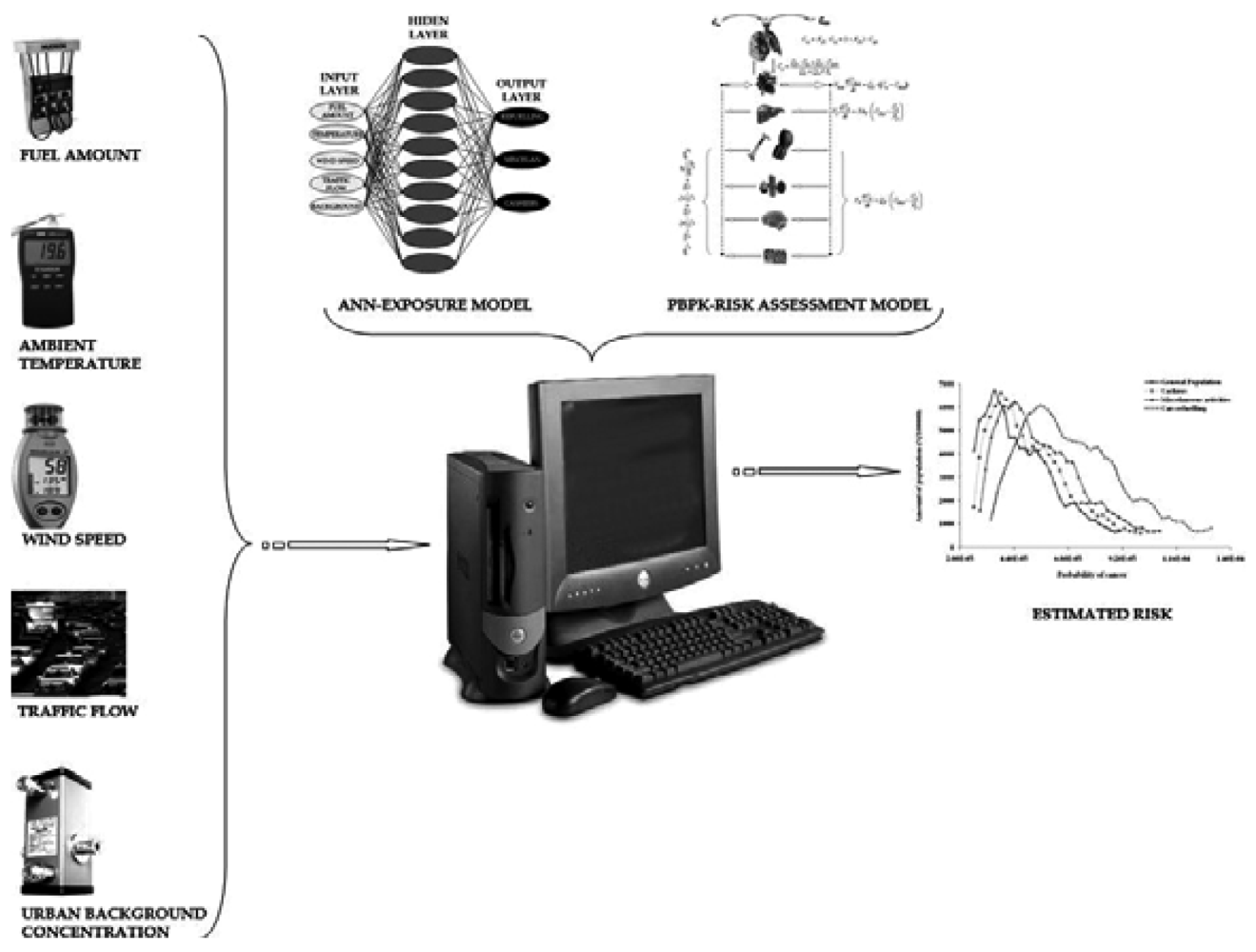
2.1. General
- -
- Gathers information from crucial environmental parameters (through the proper environmental sensors), which constitute determinants of the exposure to benzene of filling employees
- -
- Implements the proper algorithms evaluating the information obtained by the environmental sensors, in order to provide real time estimation (a) of exposure to benzene and consequently (b) of the associated health risk.
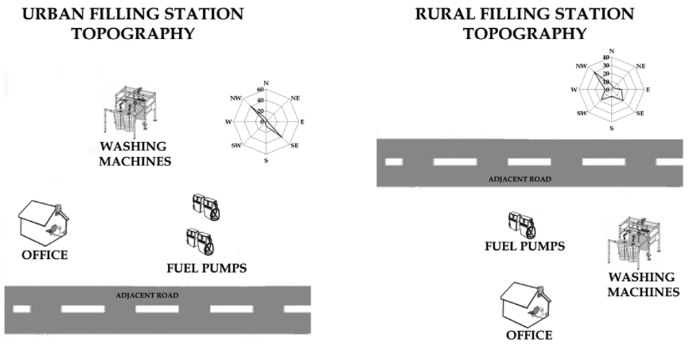
2.2. Monitoring sensor network design
- -
- The amount of the gasoline that was traded.
- -
- Wind speed (m/sec) and direction (degrees).
- -
- Ambient air temperature.
- -
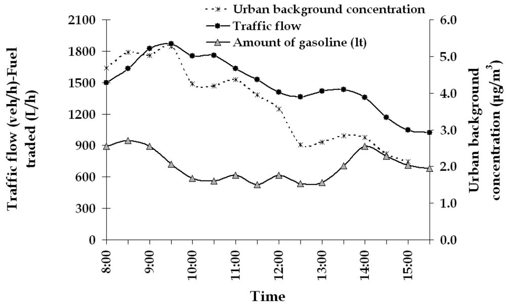
- Traffic flow from two independent observers. Vehicles were registered in seven main categories (catalytic passenger vehicles, non catalytic passenger vehicles, diesel passenger vehicles, light duty passenger vehicles, heavy duty passenger vehicles, buses and motorcycles) and the traffic volume per category was recorded every half an hour. In the urban site the measurements were continuous from 8:00 to 16:00. Vehicle speed was calculated by the quotient of the distance (a part of the road) and the time needed to cover that distance.
- -
- Urban background concentration. The most common and reliable modelling practice to define background concentration is to use data obtained from measurements at urban locations that are not directly affected by local sources [13]. Based on this, two active samplers were placed in two different urban locations (not affected by traffic or other known benzene sources) and their values were averaged in order to exclude the urban background concentration. In the rural area also two passive samplers were placed to investigate any possible background concentration or the existence of any other benzene source beside the road and the gas station emissions that may affect the measurements results. In the operational mode of a multi-sensor fusion based monitoring system as the one outlined in this study, these parameters would be measured using automated sensors and their output data streams integrated following exactly the same algorithm as the one given in this paper.
- Varian 3900 GC gas chromatography system with a flame ionization detector (FID). The capillary column through which the chromatographic separation of the various pollutants was effected, is the 30 m long, 0.53 mm inner diameter and 0.5 μm film thickness, SBM™ -5 capillary column, by Supelco, Italy.
- MARKES Thermal Desorption Cold Trap Injector thermal desorption system
- Three low volume SKC model 222 pumps for gas sampling
- DryCal CD-Lite (Bios International, USA) flow meter with a measurement range of 0.010 to 12 L/min,
- Sampling tubes (suitable both for active and passive sampling): MARKES CARBOGRAPH 5TD tubes standard absorbing cartridges filled with 400 mg of sorbent.
- Qualimetrics model 2020 and 2032 cup anemometer and wind vane, respectively.
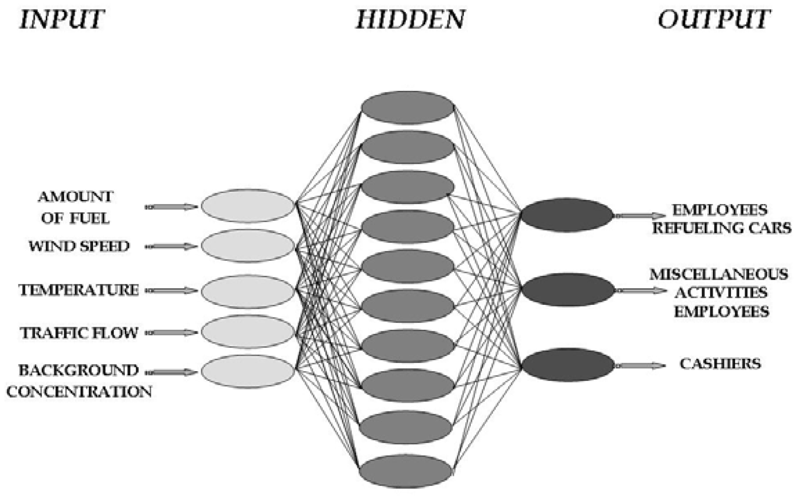
2.3. ANN (Artificial Neural Network) modeling development
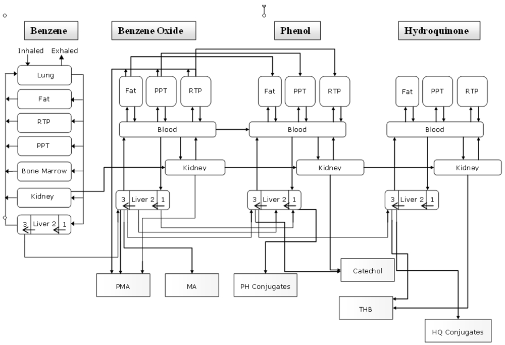
2.4. PBPK-based risk assessment model
- benzene → benzene oxide
- phenol → hydroquinone
- phenol → catechol
- hydroquinone → trihydroxy benzene
3. Results and Discussion
3.1. Traffic data
3.2. Meteorological data
3.3. Amount of gasoline traded
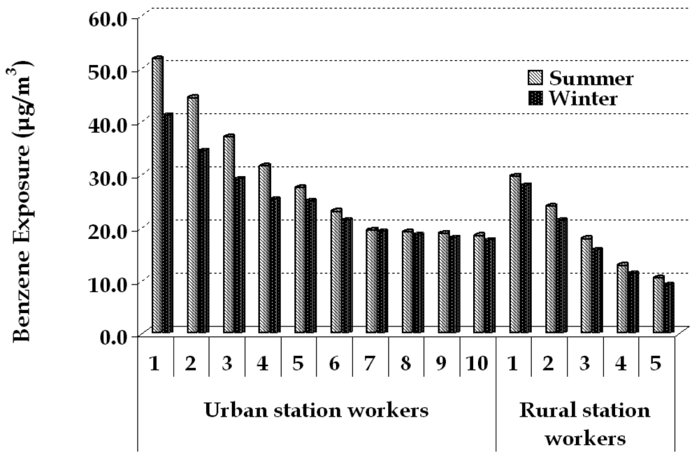
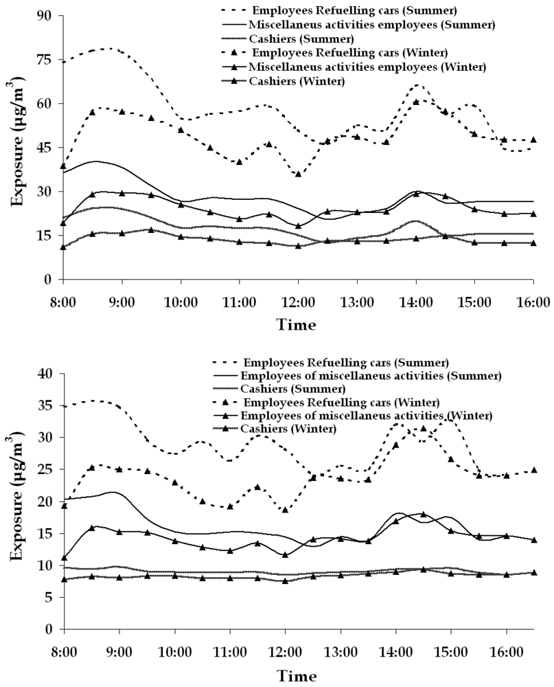
3.4. Personal exposure results
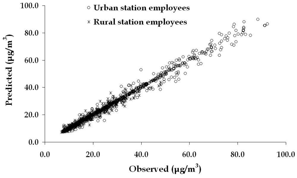
3.5. Artificial Neural Network modelling results
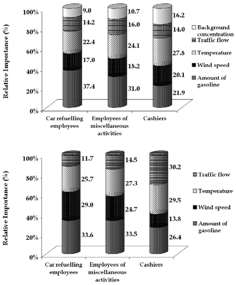
3.6. Relative importance of the parameters constituting the exposure pattern obtained by the ANN model
3.7. Potential health risk estimation
- -
- The exposure to benzene values obtained by the measurement campaign
- -
- The related concentrations of benzene metabolites on target issue (in the case of leukaemia risk this is the bone marrow) through the developed PBPK/PD model and the related dose-response curve
- -
- The variability of the population response through a Monte Carlo-Markov Chain approach
4. Conclusions
Acknowledgments
References and Notes
- Jo, W.K.; Song, K.B. Exposure to volatile organic compounds for individuals with occupations associated with potential exposure to motor vehicle exhaust and gasoline vapour emissions. Sci. Total Environ. 2001, 269, 25–37. [Google Scholar]
- IARC. IARC Monographs on the evaluation of carcinogenic risk to humans; International Agency for Research on Cancer, 2004. [Google Scholar]
- Hotz, P.; Carbonnelle, P.; Haufroid, V.; Tschopp, A.; Buchet, J.P.; Lauwerys, R. Biological monitoring of vehicle mechanics and other employees exposed to low concentrations of benzene. Int. Arch. Occ. Environ. Hea. 1997, 70, 29–40. [Google Scholar]
- Brugnone, F.; Perbellini, L.; Romeo, L.; Cerpelloni, M.; Bianchin, M.; Tonello, A. Benzene in blood as a biomarker of low level occupational exposure. Sci. Total Environ. 1999, 235, 247–252. [Google Scholar]
- Cruz-Nunez, X.; Hernandez-Solis, J.M.; Ruiz-Suareza, L.G. Evaluation of vapor recovery systems efficiency and personal exposure in service stations in Mexico City. Sci. Total Environ. 2003, 309, 59–68. [Google Scholar]
- Periago, J.F.; Zambudio, A.; Prado, C. Evaluation of environmental levels of aromatic hydrocarbons in gasoline service stations by gas chromatography. J. Chromatogr. A 1997, 778, 263–268. [Google Scholar]
- Gardner, M.W.; Dorling, S.R. Artificial neural networks (the multi-layer perceptron)- a review of applications in the atmospheric sciences. Atmos. Environ. 1998, 32, 2627–2636. [Google Scholar]
- Topouzelis, K.; Karathanassi, V.; Pavlakis, P.; Rokos, D. Detection and discrimination between oil spills and look-alike phenomena through neural networks. Int. J. Photogramm. Remote Sens. 2007, 62, 264–270. [Google Scholar]
- Gardner, M.W.; Dorling, S.R. Neural network modelling and prediction of hourly NOx and NO2 concentrations in urban air in London. Atmos. Environ. 1999, 33, 709–719. [Google Scholar]
- Karakitsios, S.; Papaloukas, C.; Kassomenos, P.; Pilidis, G. Assessment and prediction of benzene concentrations in a street canyon using artificial neural networks and deterministic models. Their response to “what if” scenarios. Ecol. Mod. 2006, 193, 253–270. [Google Scholar]
- Chiu, W.A.; Barton, H.A.; DeWoskin, R.S.; Schlosser, P.; Thompson, C.M.; Sonawane, B.; Lipscomb, J.C.; Krishnan, K. Evaluation of physiologically based pharmacokinetic models for use in risk assessment. J. Appl. Toxicol. 2007, 27, 218–237. [Google Scholar]
- Pilidis, G.; Karakitsios, S.; Kassomenos, P. BTX measurments in a medium sized European city. Atmos. Environ. 2005, 39, 6051–6065. [Google Scholar]
- Vardoulakis, S.; Fisher, E.A.B.; Pericleous, K.; Flesca, G.N. Modeling air quality in street canyons: a review. Atmos. Environ. 2003, 37, 155–182. [Google Scholar]
- MacKay, D. A practical bayesian framework for backprop networks. Neural. Comput. 1992, 4, 448–472. [Google Scholar]
- Foresee, F.D.; Hagan, M.T. Gauss-Newton approximation to Bayesian regularization. Proceedings of the IJCNN'97, Piscataway, NJ; 1997; pp. 1930–1935. [Google Scholar]
- Hagan, M.T.; Menhaj, M. Training feedforward networks with the Marquardt algorithm. IEEE Trans. Neural Networks 1995, 5, 989–993. [Google Scholar]
- Nguyen, D.; Widrow, B. Improving the learning speed of 2-layer neural networks by choosing initial values of the adaptive weights. Proc. IJCNN; Kluwer Academic: Hingham, MA, USA, 1990; 3, pp. 21–26. [Google Scholar]
- Riedmiller, M.; Braun, H. A direct adaptive method for faster backpropagation learning: The RPROP algorithm. Proc. IEEE ICNN, San Francisco, CA; 1993. [Google Scholar]
- Moller, M.F. A scaled conjugate gradient algorithm for fast supervised learning. Neural Networks 1993, 6, 525–533. [Google Scholar]
- Dennis, J.E.; Schnabel, R.B. Numerical methods for unconstrained optimization and nonlinear equations; Prentice-Hall, Inc.: Englewood Cliffs: NJ, 1983. [Google Scholar]
- Witten, I.H.; Frank, E. Data Mining: Practical Machine Learning Tools and Techniques, 2nd Ed. ed; Morgan Kaufmann: San Francisco, 2005. [Google Scholar]
- Gerlowski, L.E.; Jain, R.K. Physiologically based pharmacokinetic modeling: principles and applications. J. Pharmacol. Sci. 1983, 72, 1103–1127. [Google Scholar]
- Reddy, M.B.; Yang, R.S.; Clewell, H.J., III; Andersen, M.E. Physiologically based pharmacokinetic modelling: science and applications; John Wiley & Sons: Hoboken, NJ, 2005. [Google Scholar]
- Haddad, S.; Tardif, R.; Charest-Tardif, G.; Krishnan, K. Physiological modeling of the toxicokinetic interactions in a quaternary mixture of aromatic hydrocarbons. Tox. Appl. Pharm. 1999, 161, 249–257. [Google Scholar]
- Medinsky, M.; Kenyon, E.; Seaton, M.; Schlosser, P. Mechanistic considerations in benzene physiological model development. Environ. Health Persp. 1996, 104, 1399–1404. [Google Scholar]
- Yokley, K.; Tran, H.T.; Pekari, K.; Riihimaki, V. Physiologically-Based Pharmacokinetic Modeling of Benzene in Humans: A Bayesian Approach. Risk Anal. 2006, 26, 925–943. [Google Scholar]
- Dewaziers, I.; Cugnenc, P.H.; Yang, C.S.; Leroux, J.P.; Beaune, P.H. Cytochrome-P-450 isoenzymes, epoxide hydrolase and glutathione transferases in rat and human hepatic and extrahepatic tissues. J. Pharmacol. Exp. Ther. 1990, 253, 387–394. [Google Scholar]
- Sarigiannis, D.A. Gotti A. Biology-based dose-response models for health risk assessment of chemical mixtures. Fresenius Environ. Bull. 2008, 17, 1439–1451. [Google Scholar]
- Ntziachristos, L.; Samaras, Z. COPERT 3 – Computer programme to calculate emissions from road transport, methodology and emission factor (version 2.1); European Environment Agency: Copenhagen, Denmark, 2000. [Google Scholar]
- Pilidis, G.A.; Karakitsios, S.P.; Kassomenos, P.A.; Kazos, E.A.; Stalikas, C.D. Measurments of benzene and formaldehyde in a medium sized urban environment. Indoor/outdoor health risk implications on special population groups. Environ. Monit. Assess. 2008. [Google Scholar] [CrossRef]
- Garson, G.D. Interpreting neural-network connection weights. A.I. Exp. 1991, 6, 47–51. [Google Scholar]
- Goh, A.T.C. Back-propagation neural networks for modelling complex systems. Art. Int. Eng. 1995, 9, 143–151. [Google Scholar]
- Lan, Q.; Zhang, L.; Li, G.; Vermeulen, R.; Weinberg, R.; Dosemeci, M.; Rappaport, S.; et al. Hematotoxicity in workers exposed to low levels of benzene. Science 2004, 306, 1774. [Google Scholar]


| Urban | Rural | |
|---|---|---|
| Catalytic | 70 | 42 |
| Non catalytic | 8 | 11 |
| Diesel vehicles | 5 | 8 |
| Light duty vehicles | 7 | 23 |
| Heavy duty vehicles | 2 | 9 |
| Buses | 1 | 5 |
| Motorcycles | 7 | 2 |
| Employees refueling cars | Miscellaneous Employees | Cashiers | ||
|---|---|---|---|---|
| RRMSE | Urban | 0.0678 | 0.0352 | 0.1081 |
| Rural | 0.0880 | 0.0822 | 0.0501 | |
| Urban + Rural | 0.0900 | 0.0814 | 0.0556 | |
| R2 | Urban | 0.9729 | 0.9921 | 0.9379 |
| Rural | 0.9437 | 0.9447 | 0.8136 | |
| Urban + Rural | 0.9714 | 0.9919 | 0.9441 | |
© 2009 by the authors; licensee Molecular Diversity Preservation International, Basel, Switzerland. This article is an open access article distributed under the terms and conditions of the Creative Commons Attribution license (http://creativecommons.org/licenses/by/3.0/
Share and Cite
Sarigiannis, D.A.; Karakitsios, S.P.; Gotti, A.; Papaloukas, C.L.; Kassomenos, P.A.; Pilidis, G.A. Bayesian Algorithm Implementation in a Real Time Exposure Assessment Model on Benzene with Calculation of Associated Cancer Risks. Sensors 2009, 9, 731-755. https://doi.org/10.3390/s90200731
Sarigiannis DA, Karakitsios SP, Gotti A, Papaloukas CL, Kassomenos PA, Pilidis GA. Bayesian Algorithm Implementation in a Real Time Exposure Assessment Model on Benzene with Calculation of Associated Cancer Risks. Sensors. 2009; 9(2):731-755. https://doi.org/10.3390/s90200731
Chicago/Turabian StyleSarigiannis, Dimosthenis A., Spyros P. Karakitsios, Alberto Gotti, Costas L. Papaloukas, Pavlos A. Kassomenos, and Georgios A. Pilidis. 2009. "Bayesian Algorithm Implementation in a Real Time Exposure Assessment Model on Benzene with Calculation of Associated Cancer Risks" Sensors 9, no. 2: 731-755. https://doi.org/10.3390/s90200731