Creating Locally-Resolved Mobile-Source Emissions Inputs for Air Quality Modeling in Support of an Exposure Study in Detroit, Michigan, USA

Abstract

This work describes a methodology for modeling the impact of traffic-generated air pollutants in an urban area. This methodology presented here utilizes road network geometry, traffic volume, temporal allocation factors, fleet mixes, and emission factors to provide critical modeling inputs. These inputs, assembled from a variety of sources, are combined with meteorological inputs to generate link-based emissions for use in dispersion modeling to estimate pollutant concentration levels due to traffic. A case study implementing this methodology for a large health study is presented, including a sensitivity analysis of the modeling results reinforcing the importance of model inputs and identify those having greater relative impact, such as fleet mix. In addition, an example use of local measurements of fleet activity to supplement model inputs is described, and its impacts to the model outputs are discussed. We conclude that with detailed model inputs supported by local traffic measurements and meteorology, it is possible to capture the spatial and temporal patterns needed to accurately estimate exposure from traffic-related pollutants.

1. Introduction

A recent World Health Organization report [1] linked more than seven million deaths in 2012 to air pollution, making it the largest single environmental health risk. With the large number of people exposed to high levels of air pollution in urban areas, there is an increasing need to have highly resolved spatiotemporal modeling tools to capture high exposure levels for health studies, and to link sources of emissions with their adverse health effects. Mobile sources are key contributors to adverse air pollution impacts, because of their prevalence and proximity to the exposed populations.

Air quality models have traditionally provided critical information for air quality management decisions, but recently have also been used to provide exposure estimates for air pollution health effects studies. Dispersion models can be challenging to implement, particularly in studies addressing near-road impacts, due to the detailed inputs needed to estimate traffic-related emissions [2]. The methodology and example case study presented here provide information on some of the data needed to model traffic-related pollutant impacts accurately in a large, diverse urban area.

Modeling the dispersion of traffic-generated air pollutants requires pollutant emissions estimates, which are typically obtained based on one of two approaches. A top-down approach utilizes population- or activity-based spatial surrogates to allocate emissions from a county level to grid squares. This approach can be adequate on a large scale, but in an urban area where the distance from a roadway source in increments of tens of meters is an analysis metric, more resolution is needed in the near-field [3], so a bottom-up approach is more appropriate. A bottom-up approach requires detailed information, such as the geometry of the road network, traffic volumes, temporal allocation factors, fleet mixes (the distribution of vehicle classes), and pollutant-specific emission factors. Assembled from a variety of sources, this information is combined with meteorological inputs to generate link-based (straight-line representation of roadway segments) emissions for use in dispersion modeling to estimate pollutant concentrations due to traffic.

The main objective of this analysis is to present a bottom-up emissions estimation methodology that we developed as an approach for estimating near-field exposure to traffic-generated pollutants in Detroit, MI, in support of the Near-Road Exposure and Effects of Urban Air Pollutants Study (NEXUS) [4]. Thus, this study is a part of a series of papers related to the NEXUS study, where model based exposure metrics were used to determine exposures for all participants throughout the study period. These exposure metrics were a complement to measured air quality concentrations when personal, ambient, and location specific measurements were not feasible for the entire study period for all participants. Although the NEXUS study extended over three years, for our intensive analysis to illustrate the methodology, we selected three months: fall (August–October) of 2010. The intensive analysis was designed to demonstrate the capability of modeled air quality to be used as indicators of exposure to traffic based on traffic patterns and hourly meteorology. This analysis included a cohort of 160 asthmatic children selected based on the proximity of their primary residence to high-traffic roadways. In NEXUS, some limited measurements were taken at participant home locations for short time periods throughout the study, as well as at their school locations throughout the whole study period. These measurements are a combination of contributions from mobile, industrial, and background sources. As a part of this study air quality estimates were produced for all source types and combined to provide a total modeled exposure metric. This work is presented in companion papers by Aranachalam et al. [5] and Isakov et al. [6]. Here we extensively analyze the mobile source component of the total predicted concentrations that went into the exposure metric analysis by Batterman et al. [7].

Air quality estimates due to mobile sources are obtained using an estimated hourly emission for each roadway and a dispersion concentration from the roadway to each receptor. This method involves a decoupled approach to estimate emissions and dispersion, where each piece can be estimated and analyzed independently before assessing the combination of the two. In the following sections, we begin with presenting a methodology to generate link-based emissions followed by applying a line source dispersion model to a complex urban area. We then present results from our sensitivity analysis of the emissions and dispersion components separately. After presenting the methodology and sensitivity analysis of the emissions and dispersion estimates we present results of the full combined methodology to a health study in Detroit, MI. Finally, we explore using local traffic measurements to adjust activity that was obtained by the travel demand model. We explain how this changes the emission estimates and then present an analysis of the revised results. We conclude the results section by highlighting the implications that these local measurements have on the modeled mobile source air quality estimates.

2. Methodology for Estimating Near-Road Air Quality Concentrations

Emissions outputs are generated by combining readily available local data, national default data, and travel demand model (TDM) outputs to obtain a link-based emission for each vehicle class on each roadway. We describe below these inputs and the method we developed for combining them. Throughout this section a large number of acronyms are defined and used, we have included all acronyms/abbreviations in Table S1 of the supplemental material.

The total emission factors, $E{F}_i$ (grams/vehicle/mile), and traffic activity, $A_i$ (vehicles), are combined to create hourly emissions, $E_i$(grams/mile), for each road link, i, in the road network:

$$E_i=E{F}_i\times A_i$$

(1)

where:

$$E{F}_i={\displaystyle \sum }_{veh.class}e{f}_i\left(pollutant, speed, month, temperature\right)\times fleet mix\left(vehicle class\right)$$

(2)

in which $ef$ is the vehicle-class-specific emission factor, and fleet mix is the fraction of vehicle class activity relative to the total fleet; and where:

$$A_i=AAD{T}_i\times TA{F}_i(\mathrm{h}\mathrm{o}\mathrm{u}\mathrm{r}, \mathrm{d}\mathrm{a}\mathrm{y}, \mathrm{m}\mathrm{o}\mathrm{n}\mathrm{t}\mathrm{h})$$

(3)

in which $AAD{T}_i$ is the average annual daily traffic and $TA{F}_i$ is the temporal allocation factor. The total concentration is then computed by:

$$C= {\displaystyle \sum }_i{E}_i\times {\chi }_i$$

(4)

where ${\chi }_i$ is the unit concentration in μg/m³ from each road link, i, to each receptor.

The above method allows the emission and dispersion models to be run independently from one another. We used R-LINE [8], a research-grade line-source dispersion model to calculate the dispersion of pollutants from each road link to each receptor; this modeling is done using a unit emission rate (1 g/m/s). Emissions data are then computed separately for each road link for every hour of the year in g/m/s, and these data are applied as scaling factors to the dispersion model results using unit emission factors. Concentrations are modeled for each receptor for every hour of the year. This two-step process allows emissions adjustments to be applied easily, if needed, thus avoiding time-consuming reruns of the dispersion model. In the NEXUS study, we found that local measurements showed slightly different annual average daily traffic (AADT) counts for some roadways compared to the traffic counts obtained from the travel demand model, a model typically used to estimate vehicle travel on roadways in an urban area. Using local measurements we were able to easily adjust for this and recompute the emissions, then combine these revised outputs with the previously computed unit emission based dispersion concentrations. This process will be discussed in Section 4.2.

2.1. Estimating Link-Based Emissions Using an Urban Road Network, Traffic Activity Estimates, and Emission Factors.

For our study we are estimating impacts of roadways on a highly resolved spatial extent, from 25 to a few hundred meters. These highly resolved emissions estimates are needed to appropriately model roadway impacts. A bottom-up approach was used to estimate hourly emissions on individual roadlinks where local information including road links, traffic volumes, and fleet mixes are used to obtain link-based emissions for the entire study domain. These emissions are combined with dispersion model results to obtain pollutant concentrations at each model receptor (e.g., the location of a NEXUS participant’s home). This process for generating mobile-source emissions and pollutant concentrations is described below, using Detroit as a case study.

The national functional class (NFC) system [9] is used by the Federal Highway Administration (FHWA) to designate road type; these designations and descriptions are shown in Table 1.

Table 1. National functional class roadway descriptions for urban roadways.

Description	NFC
Urban Interstate (Principal Arterial)	11
Urban Other Freeway (Principal Arterial)	12
Urban Other Principal Arterial	14
Urban Minor Arterial	16
Urban Collector	17
Urban Local	19

Table 1. National functional class roadway descriptions for urban roadways.

Description	NFC
Urban Interstate (Principal Arterial)	11
Urban Other Freeway (Principal Arterial)	12
Urban Other Principal Arterial	14
Urban Minor Arterial	16
Urban Collector	17
Urban Local	19

A map of the Detroit area illustrating the NFCs is shown in Figure S1 in the Supplementary Material (note that within the chosen domain, only the urban NFCs were present in the Southeast Michigan Council of Governments (SEMCOG) database we used) In this study, we used fleet mix and activity data for over 9000 road links with multiple roadway classifications.

The traffic activity estimates for Detroit were obtained from the SEMCOG [10]. These estimates were generated by combining spot traffic counts with TDM outputs and vehicle mileage reports to obtain the average annual daily traffic and speeds for major road links in the Detroit network. We do not include the smaller neighborhood streets in our modeling, because of low intermittent traffic volumes and emissions on them.

From the TDM we obtained speeds for the five time periods of the day shown in Table 2. The speeds in the two off-peak time periods were assumed to be the same.

Table 2. Modeled time periods of day for determining speed and estimating exposure.

Time Period	Hours of Day (Local)
Off-peak1	12:00 AM–6:59 AM
AM-peak	7:00 AM–8:59 AM
Mid-day	9:00 AM–3:59 PM
PM-peak	4:00 PM–6:59 PM
Off-peak2	7:00 PM–11:59 PM

Table 2. Modeled time periods of day for determining speed and estimating exposure.

Time Period	Hours of Day (Local)
Off-peak1	12:00 AM–6:59 AM
AM-peak	7:00 AM–8:59 AM
Mid-day	9:00 AM–3:59 PM
PM-peak	4:00 PM–6:59 PM
Off-peak2	7:00 PM–11:59 PM

The AADT and speeds on road links in the Detroit domain are shown in Figure 1 and Figure 2, respectively.

Figure 1. The AADT for road links in the Detroit domain.

Figure 1. The AADT for road links in the Detroit domain.

Figure 2. The average speed on each road link in the Detroit domain.

Figure 2. The average speed on each road link in the Detroit domain.

To create hourly traffic volumes, we multiplied the AADT by the temporal allocation factors (TAFs) from the 2008 National Emissions Inventory [11], which are hourly factors that create traffic volume patterns. We began with a general approach to test our methodology by using national default TAFs. Although patterns can vary geographically, this would be the general approach that would be used in this region.

The hourly TAFs for weekdays have a bimodal pattern to represent the high-traffic periods of the morning and evening rush hours (7–8 AM and 5–6 PM). In contrast, weekend traffic patterns are single-mode, with the maximum traffic at 4 PM. Also, a day-of-the-week traffic pattern is used to represent higher traffic volume during the week and smaller traffic volumes on the weekend. Finally, monthly traffic patterns are utilized to represent the higher summer travel period and lower winter travel period. All of these TAFs are presented in the Supplementary Material (Figure S2).

We ran the Motor Vehicle Emissions Simulator (MOVES) 2010 (Version 2010b) [12] in rate-per-distance mode on the county-level scale with hourly time aggregation for each of the three counties in the study area (Wayne, Oakland, and Macomb). Consistent with Cook et al. [3], we calculated emissions factors (EFs) for multiple pollutants—including PM₁₀, PM_2.5, EC₁₀ (or BC₁₀), EC_2.5 (or BC_2.5), OC₁₀, OC_2.5, SO₄, NO_x, SO₂, CO, and benzene—from the running exhaust and running evaporative modes. In addition, brakewear and tirewear modes were factored into the PM emissions. Where possible, local input data obtained from SEMCOG were used in place of the default input data; these local data included fleet mixes and fuel properties (the blend of fuels used by each type of vehicle), as well as typical monthly temperature and relative humidity values derived from the nearby National Weather Service (NWS) station. We then post-processed the raw MOVES outputs to create annual EF tables organized by month (January–December), pollutant, vehicle type, temperature (from 0^° to 100 ^°F by 10 ^°F increments), and speed in miles per hour (2.5 mph, then from 5 mph to 75 mph by 5-mph increments), with one line per month/temperature/speed combination. An example set of emissions for the month of August 2010 for a temperature of 50 ^°F and a speed of 45 mph is plotted in Figures S3 and S4 in the Supplementary Material. We used hourly temperatures from meteorological data collected at a local airport to determine the hourly emission factors for each road link.

We determined the fleet mixes by starting with the 2010 FHWA highway statistics for Michigan [13], which break down traffic volume into six Highway Performance Monitoring System (HPMS) vehicle types (motorcycles, passenger cars, light trucks, buses, single-unit trucks, and combination trucks) for urban and rural interstates, arterials, and other road types (collectors and locals). These vehicle classes are further broken down into the eight vehicle classes shown in Table 3, using the U.S. Environmental Protection Agency (EPA) guidance by Decker et al. [14] mapping HPMS to MOBILE5A vehicle categories (the same mapping used by MOVES). Once we combined these sources, we were able to find fleet mixes by vehicle type for the MOVES roadway classes shown in Table 1. Our fleet-mix results are summarized for urban roadways in Table 4 (as noted earlier, only urban NFCs were present in the SEMCOG database for the Detroit region of interest).

Table 3. Vehicle types by fuel and abbreviations.

Fuel	Vehicle Type	Abbreviation
Gasoline	Light-Duty Gasoline Vehicles	LDGV
	Light-Duty Gasoline Trucks1	LDGT1
	Light-Duty Gasoline Trucks2	LDGT2
	Heavy-Duty Gasoline Vehicles	HDGV
	Motorcycles	MC
Diesel	Light-Duty Diesel Vehicles	LDDV
	Light-Duty Diesel Trucks	LDDT
	Heavy-Duty Diesel Vehicles	HDDV

Table 3. Vehicle types by fuel and abbreviations.

Fuel	Vehicle Type	Abbreviation
Gasoline	Light-Duty Gasoline Vehicles	LDGV
	Light-Duty Gasoline Trucks1	LDGT1
	Light-Duty Gasoline Trucks2	LDGT2
	Heavy-Duty Gasoline Vehicles	HDGV
	Motorcycles	MC
Diesel	Light-Duty Diesel Vehicles	LDDV
	Light-Duty Diesel Trucks	LDDT
	Heavy-Duty Diesel Vehicles	HDDV

Table 4. Fleet-mix results for urban roadways in Detroit, MI (percentages), USA.

Fuel	Vehicle Type	Interstate NFC 11	Arterials NFC 12, 14, 16	Other NFC 17, 19
Gasoline	LDGV	70.82	75.66	50.50
	LDGT1	11.59	11.08	24.98
	LDGT2	5.90	5.64	12.72
	HDGV	2.21	2.20	1.15
	MC	0.40	0.20	2.10
Diesel	LDDV	0.98	1.04	0.70
	LDDT	0.51	0.49	1.09
	HDDV	7.69	3.70	6.75

Table 4. Fleet-mix results for urban roadways in Detroit, MI (percentages), USA.

Fuel	Vehicle Type	Interstate NFC 11	Arterials NFC 12, 14, 16	Other NFC 17, 19
Gasoline	LDGV	70.82	75.66	50.50
	LDGT1	11.59	11.08	24.98
	LDGT2	5.90	5.64	12.72
	HDGV	2.21	2.20	1.15
	MC	0.40	0.20	2.10
Diesel	LDDV	0.98	1.04	0.70
	LDDT	0.51	0.49	1.09
	HDDV	7.69	3.70	6.75

When all of these inputs are combined, they give hourly emissions for each road link in the Detroit domain. The emissions vary by temperature, time of day, month of year, day of week, and roadway speed. Figure 3 gives example emissions results for August 2010 at a temperature of 50 ^°F for the average hourly emissions during the AM-peak time period.

Figure 3. Emissions results (in g/h) for Detroit road links for an average AM-peak hour in August 2010: emissions of PM_2.5 (top panels) and of CO (bottom panels). The right-hand panels show an enlargement of downtown.

Figure 3. Emissions results (in g/h) for Detroit road links for an average AM-peak hour in August 2010: emissions of PM_2.5 (top panels) and of CO (bottom panels). The right-hand panels show an enlargement of downtown.

Figure 3 demonstrates the emission resolution of this modeling methodology. Major roadways (from Figure 1 and Figure 2: AADT > 50,000 and speeds > 40 miles per hour,) appear to have the highest emissions of PM_2.5 and CO. Smaller arterial roadways (with AADT < 20,000 and speeds < 30 miles per hour, from Figure 1 and Figure 2) have 10% of the emissions of the major roadways.

2.2. Using a Dispersion Model for Line Sources

A research dispersion model for line sources (R-LINE) was developed by EPA’s Office of Research and Development [8]. This model is a research platform to study dispersion from roadways in various atmospheric conditions with various near-road complexities. R-LINE is currently designed for flat roadways, without depressions or noise barriers; further development is ongoing to address these near-road complexities. In the NEXUS study, this model was applied as if all roadways are at-grade without road complexities. The model uses the locally observed hourly meteorology and applies wind profiling to simulate turbulence effects of the urban area when modeling dispersion plumes from all road links.

Using local meteorology allows R-LINE to correctly model the dispersion of roadway emissions to determine meteorological causes for increases in air pollution on temporally and spatially resolved scales. The NEXUS study looked at both acute and long-term symptoms of exposure to high traffic roadways with two levels of diesel traffic. The dispersion model is capable of predicting high impact days and even hours of high exposure created by hourly meteorology [8] to assess acute impacts. This amount of temporal resolution is not possible using traditional land use regression (LUR)-based models, which produce long-term average exposures and have only recently been extended to hourly resolution, but with increased uncertainties [15].

We computed exposure estimates by combining hourly emissions and dispersion estimates developed using unit emission rates. To analyze the combined results we performed a brief sensitivity analysis of the dispersion model outputs to the meteorological inputs in Section 3.2.

3. Sensitivity of Emissions and Dispersion Estimates to Inputs

Section 2 describes a methodology for producing emissions estimates and dispersion estimates separately and combining them to create air quality estimates for mobile source impacts in an urban area. In this section we present limited sensitivity analyses of the emission and dispersion estimates to some of their inputs; these sensitivities provide additional information for the results of their combination, which are shown in Section 4. Again, a large number of acronyms are defined and used in this section, we have included all acronyms/abbreviations in Table S1 of the supplemental material.

3.1. Sensitivity of Emissions Estimates to Roadway Type

In estimating the exposure metrics for the NEXUS study, we modeled all major roadways in the Detroit area. Comparison between Figure 3 and the NFC designation (Figure S1), shows the highest emissions are from NFC 11 and 12 roadways. An integral part of the NEXUS health study hypotheses is based around the impact of diesel traffic, thus a distinction between the exposure from high-diesel and low-diesel roadways, these are modeled as NFC 11 and 12 roadways, respectively. In order to have this distinction between high and low diesel roadways there must be a clear distinction in the emissions inputs, thus we look at the sensitivity of emissions to the roadway type.

In Detroit, the interstates are always designated as NFC 11 and represent high-diesel (HD) roadways, while the freeways are designated as NFC 12 and represent low-diesel (LD) roadways. Here we focused on Detroit NFC 11 and NFC 12 roadways in August 2010.

The first comparison of inputs between the two roadway types is vehicle speed for the five time periods of the day shown in Table 1. Roadway speeds are assumed to be the same for all vehicle types on the roadway. Analysis of the speed variation among these time periods showed that the speeds for each link did not differ by more than 10 mph across the time periods, which is the resolution of the speed bins in the emission factor tables. In addition, the average speeds for NFC 11 and NFC 12 roadways were 48 and 46 mph, respectively, which are in the same 10-mile per hour speed bin for the MOVES emissions factors; thus they will have the same emissions in grams per vehicle per mile.

The next comparison of inputs is for the fleet mix. As Lindhjem et al. [16] have shown, the fleet mix is a major contributor to the total emissions profiles for specific roadways as well as the entire roadway network. From Table 4, summing the HDDV, LDDT, and LDDV yields a diesel vehicle percentage of 9.18% for NFC 11 roadways and 5.23% for NFC 12 roadways. We computed ratios for primary roadway pollutant emissions from NFC 11 to NFC 12 roadways (Table 5), where the only difference is the fleet mix; the weighting factors for day of week, hour of day, or month of year are not considered, because these would be the same for both roadway types.

Table 5. The ratio of primary pollutant emissions from interstates (HD) and freeways (LD) based on the fleet mix for Detroit, MI, MOVES emissions tables for August 2010.

Primary Pollutant	PM2.5	NOx	CO
HD/LD ratio	1.53	1.29	0.94

Table 5. The ratio of primary pollutant emissions from interstates (HD) and freeways (LD) based on the fleet mix for Detroit, MI, MOVES emissions tables for August 2010.

Primary Pollutant	PM2.5	NOx	CO
HD/LD ratio	1.53	1.29	0.94

Table 5 indicates that pollutants with larger emission rates from diesel vehicles (HD) are the most affected by fleet mix. Primary PM_2.5 shows the largest effect (furthest from 1.0); this is consistent with source apportionment studies such as Gertler [17]. Primary NO_x shows less of an impact from diesel traffic, but still could be significant in exposure estimates. Carbon monoxide, on the other hand, shows virtually no effect (closest to 1.0) based on fleet mix. The level of CO emissions is an indicator of the total traffic on a roadway; the magnitude indicates the amount of emission from a roadway, not the composition of the vehicles traveling it.

Although we used the average speed for the two roadway types, it is important to note that there is a large variation within each NFC grouping of road links (as much as 45 mph). This large difference in speed will give vastly different emission factors per vehicle, especially for diesel vehicles, which are more prevalent on NFC 11 roadways. The lower-speed links are typically on and off ramps from freeways and interstates, which would produce higher emissions per vehicle in all vehicle classes for most pollutants.

Because pollutant concentration estimates are produced by direct multiplication of the emissions and the dispersion based on unit emissions estimates (as described above), the large differences in some primary pollutant emissions translate directly to differences in concentration estimates due to mobile sources.

The detailed emissions differences between roadway types highlight the importance of designating the roadways correctly in order to accurately represent each roadway’s diesel percentage. Incorrect NFC designation between classes 11 and 12 could result in as much as 53% error in the estimated PM_2.5 concentration (as shown in Table 5). This type of error in pollutant concentration could lead to incorrect conclusions and correlations between exposure metrics and health outcomes. As we conducted our study, we saw that in some cases roadways with the same NFC designation had very different diesel traffic percentages in traffic counter data. We therefore redesignated several roads to better represent measured diesel percentages; this adjustment is discussed in Section 4.2.

3.2. Sensitivity of Dispersion Model Results to Meteorological Inputs

Hourly meteorological parameters are used to drive dispersion models, which produce hourly variations in dispersion from emission sources. Dispersion model outputs are dependent on model inputs. Thus we constructed a sensitivity analysis for representative dispersion hours in the Detroit region. These dispersion concentrations from the meteorology sensitivity analysis were combined with emissions to determine pollutant concentrations for all study participants.

Meteorological inputs were applied to all roadways for the study period to obtain long-term and acute variations in air-quality due to roadway sources. For a study to address long and short-term health impacts, a complete and consistent meteorological dataset is needed. We examined meteorology from multiple airports in the region, but focused on two airports in the city of Detroit. We compared meteorological measurements at two Detroit Airports, Detroit City (DET) and Detroit Metro (DTX); DET is located north and east of the urban center, DTX is located south and west of the city center. Comparison of parameters such as wind speed, wind direction, stability, and surface roughness between the airports gave us confidence that the meteorological trends throughout the study period are seen throughout the study domain. The meteorology for the DET airport was selected as representative of the study participants because it had a greater number of valid meteorological measurements throughout the period, and it is located near the middle of the study domain in a suburban area that is representative of the suburban neighborhoods where the participants’ homes are located.

Figure 4 shows a wind rose of the measured values at DET for fall 2010, the NEXUS period we selected for our intensive analysis. The prevailing wind is from the northwest and blows toward the southeast. There are also many low speeds when wind is coming from the southeast.

Figure 4. Wind rose for Detroit City Airport during the fall 2010 period, with wind speeds in meters per second. Paddles show the direction from which the wind is originating as it blows over the Detroit area.

Figure 4. Wind rose for Detroit City Airport during the fall 2010 period, with wind speeds in meters per second. Paddles show the direction from which the wind is originating as it blows over the Detroit area.

To examine the influence of atmospheric stability, we selected four hours that represent four distinct stability conditions (see Table 6): neutral (|L| > 500 m), stable (100 m < L ≤ 500 m), very stable (1 m < L ≤ 100 m), and convective (−500 m ≤ L < −1 m). These four conditions represent the amount of turbulence and mixing present in the atmospheric boundary layer created by wind speed and heat exchange between the Earth’s surface and the lower layers of the atmosphere; convective conditions mean the most turbulence and heat exchange, stable conditions mean the least turbulence and heat exchange, and neutral conditions are somewhere in between stable and convective. Key meteorological parameters used by R-LINE are the friction velocity (u *), the convective mixing height (z_ic), the mechanical mixing height (z_im), the Monin-Obukhov length (L), the roughness length (z₀), and the wind speed (u), and we present these variables for the various stability conditions in Table 6.

Table 6. Representative meteorological conditions from fall 2010 for Detroit, MI, USA.

Condition	u * (m/s)	zic (m)	zim (m)	L (m)	z0 (m)	u (m/s)
Convective	0.229	80	252	−12.9	0.167	1.65
Neutral	0.734	356	1445	−1223.7	0.48	4.63
Stable	0.254	N/A	294	104.5	0.104	2.66
Very Stable	0.093	N/A	137	12.8	0.104	1.03

Table 6. Representative meteorological conditions from fall 2010 for Detroit, MI, USA.

Condition	u * (m/s)	zic (m)	zim (m)	L (m)	z0 (m)	u (m/s)
Convective	0.229	80	252	−12.9	0.167	1.65
Neutral	0.734	356	1445	−1223.7	0.48	4.63
Stable	0.254	N/A	294	104.5	0.104	2.66
Very Stable	0.093	N/A	137	12.8	0.104	1.03

R-LINE was run using unit emissions and the wind perpendicular to the roadway for each of the representative meteorological hours. Concentration results are shown in Figure 5. The drop in concentration as a function of distance from the roadway shows that the stable and very stable meteorological conditions have the highest impact in terms of pollutant exposures. For convective and neutral meteorological conditions, the results show very little (<10%) difference in concentrations for all downwind distances of the roadway. Also notice that upwind concentrations are shown as negative downwind distances, and are nonzero near the roadway; this indicates that the wind direction and receptor location are important factors in analyzing estimated dispersion concentration gradients.

The meteorological parameters used to model dispersion are interdependent and were calculated using AERMET [18] based on one-minute sonic anemometer measurements of meteorological parameters at DET’s Automated Surface Observing System (ASOS). An analysis of the one-minute measurements from this meteorological site revealed that on average there was only a 20% standard deviation in the mean hourly wind speed during the fall 2010 period. This small variation in wind speed throughout the hour provides confidence in the meteorological parameters used as inputs to R‑LINE and the statistical basis of Gaussian dispersion theory used to determine hourly concentration estimates.

During this calculation process the atmospheric stability is determined by measurements of heat flux, so the difference between stable, convective, and neutral conditions is well known. However, it is more difficult to discern the degree of the atmospheric stability from direct measurements, so an interdependent iterative calculation is used that is based on the reference wind speed, calculated wind profile, estimated surface roughness, and measured heat flux. This process yields the Monin-Obukhov length, L, which is a measure of the atmospheric turbulent length scale.

Figure 5. R-LINE concentration gradients for the representative meteorological conditions in Table 6. All concentrations are normalized by the estimated concentration closest to the roadway

Figure 5. R-LINE concentration gradients for the representative meteorological conditions in Table 6. All concentrations are normalized by the estimated concentration closest to the roadway

The differences in concentration fall-off shown in Figure 5 emphasize the importance of using accurate surface meteorological parameters in modeling for all conditions, but especially for stable conditions, where there can be a large range of concentrations between stable and very stable meteorological hours; the severity of stability is determined by measurements of heat flux and surface roughness. The very stable hours typically occur during the early morning hours and usually last through the morning rush hour. The combination of a stable atmosphere and high roadway emissions leads to the potential for extremely high exposures to traffic-related pollutants during the rush hour.

4. Results

In the previous section we presented emissions sensitivities due to model inputs and example dispersion characteristics to aid in the interpretation of the modeled concentrations, which are a linear combination of the emission and dispersion estimates. We applied the methodology described in Section 2 for all road links in the Detroit area for a set of 160 NEXUS study participants’ home locations. These runs are referred to as the base-case simulation. Then we used local measurements of traffic to modify our estimation of emissions and examined the resulting impacts on the exposure estimates for the same locations and examine the implications of using local measurements to augment the methodology for the application in the NEXUS health study.

4.1. Base-Case Simulations

For this model run we used our unit emission rate dispersion results and the emissions inputs generated as described in Section 2.1, and analyzed the resulting modeled concentrations for the fall 2010 period. We reduced the number of points to analyze by calculating average hourly concentrations or exposure metrics by time of day for each of the time periods shown in Table 2 on each day of the study period. These outputs were calculated using valid meteorological hours for each time period with a 75% completeness criterion; this is needed because missing concentrations occur when the wind speed is less than 0.5 m/s or the instruments did not record a complete set of measurements. 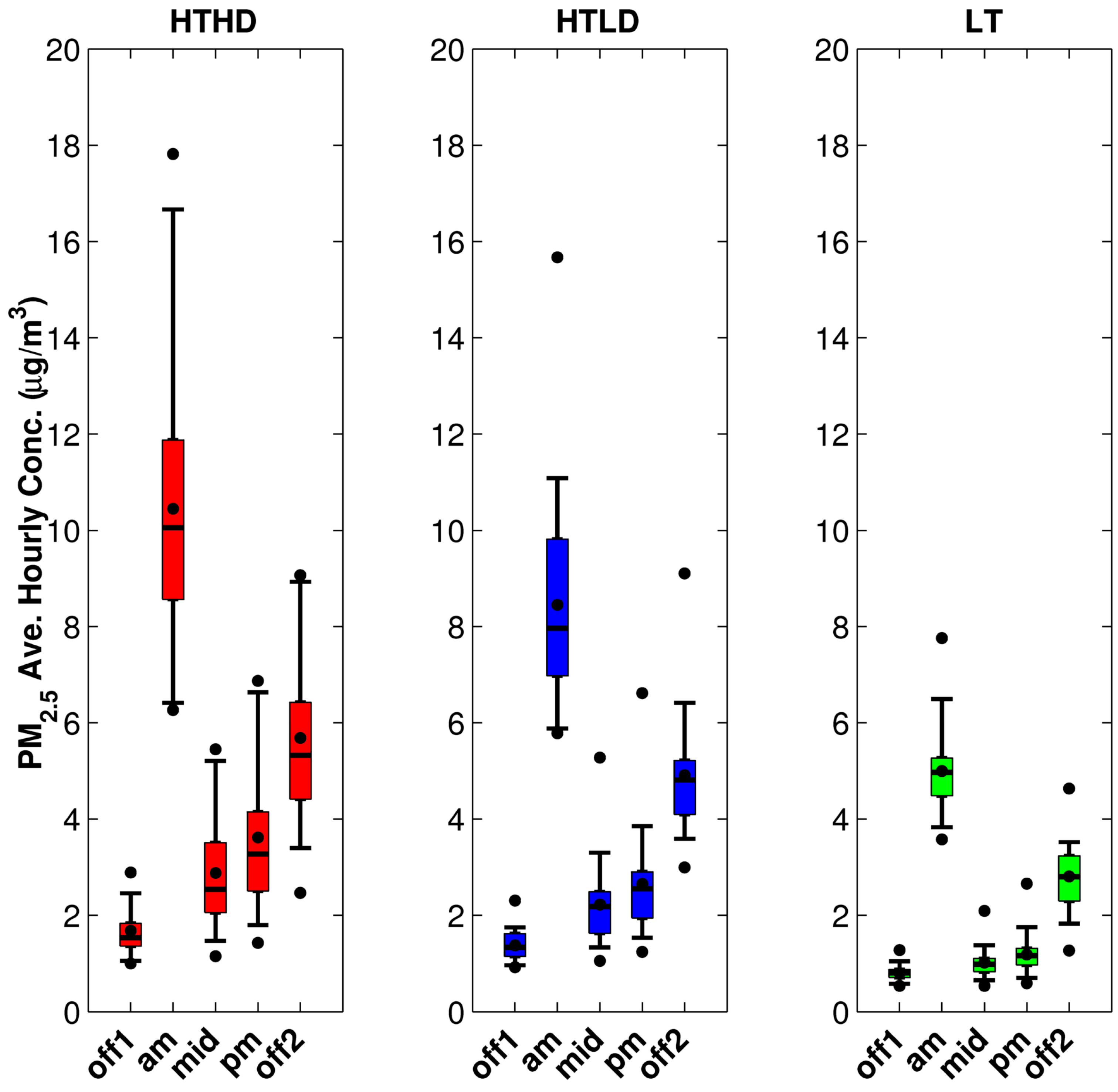The temporal pattern is illustrated in Figure 6 for PM_2.5 concentrations from mobile sources at participants’ home locations. The participants’ home locations were described as within 300 m of HTHD roadways, within 300 m of HTLD roadways, or beyond 300m from HTHD and HTLD roadways. We also calculated the average hourly concentration for the entire day using the same completeness criterion. 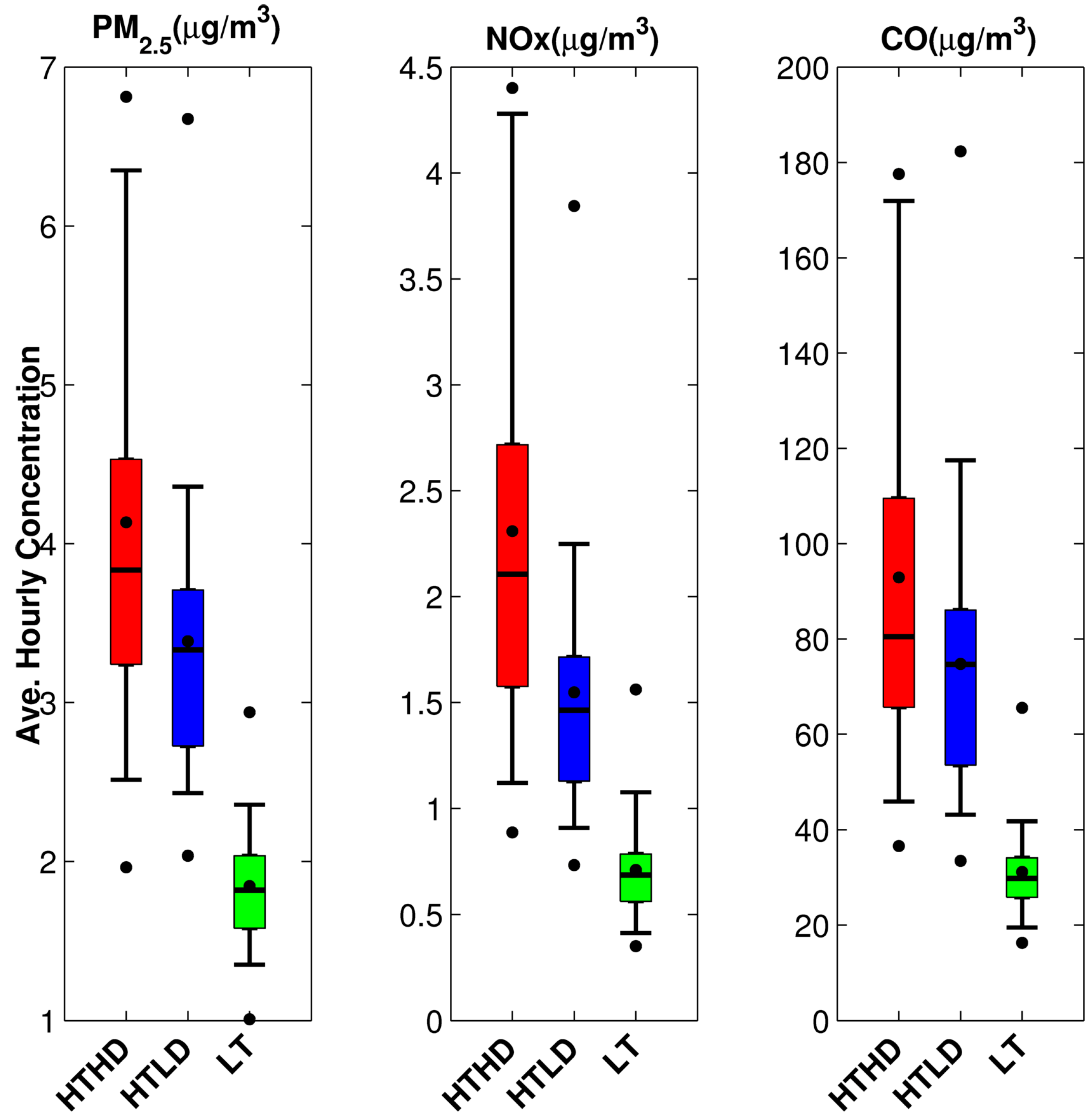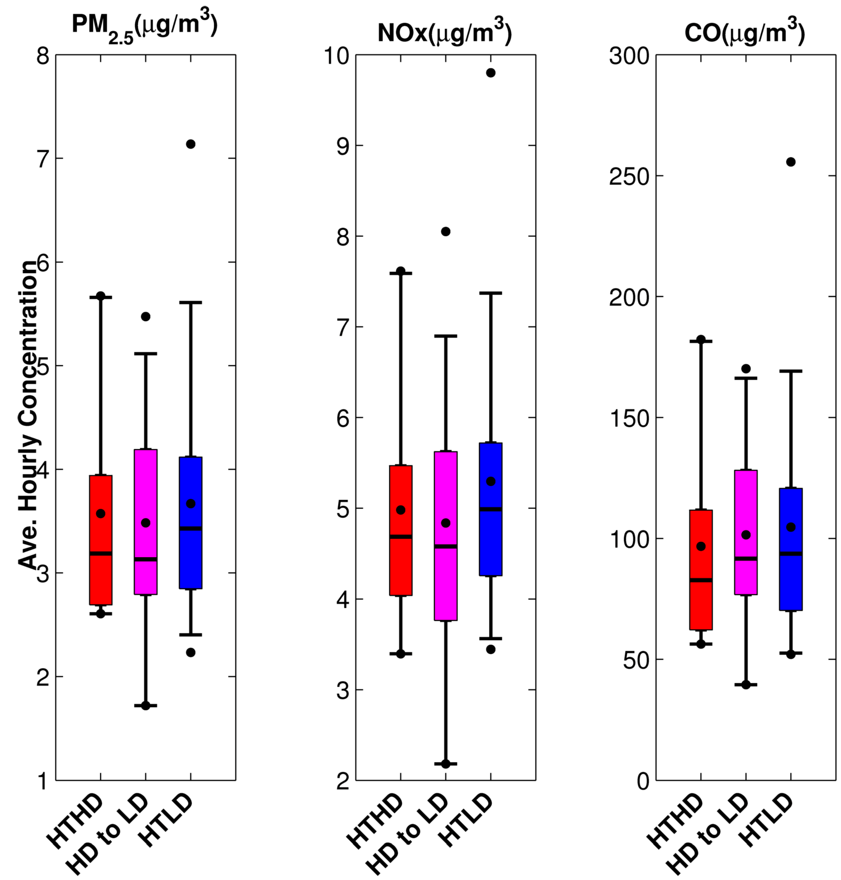Figure 7 shows the daily average hourly concentration for PM_2.5, NO_x, and CO.

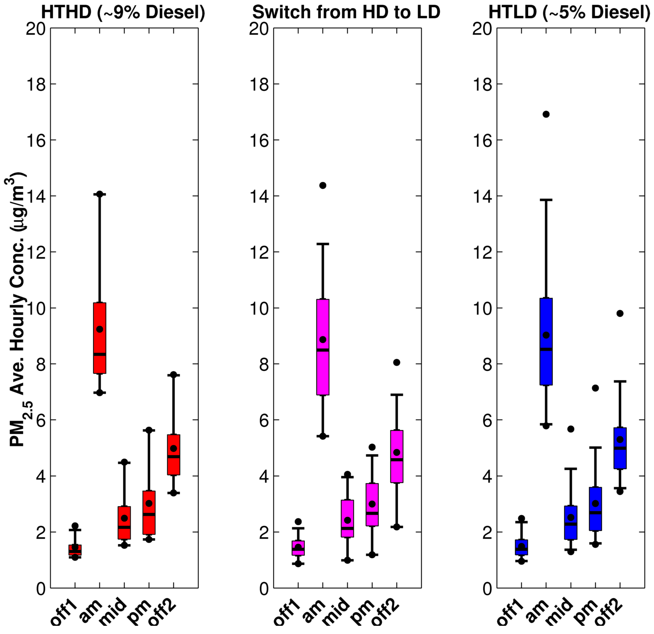
Figure 6. Temporal distributions of mobile-source component of PM_2.5 concentration for the fall 2010 period, separated into high-traffic, high-diesel (HTHD), high-traffic, low-diesel (HTLD), and low-traffic (LT) participant home locations. The box represents the middle 50% of measurements, and the median is the horizontal line in the middle; the whiskers represent the 5th and 95th percentile; and the dots represent the minimum, mean, and maximum. Time periods are defined in Table 2.

Figure 6. Temporal distributions of mobile-source component of PM_2.5 concentration for the fall 2010 period, separated into high-traffic, high-diesel (HTHD), high-traffic, low-diesel (HTLD), and low-traffic (LT) participant home locations. The box represents the middle 50% of measurements, and the median is the horizontal line in the middle; the whiskers represent the 5th and 95th percentile; and the dots represent the minimum, mean, and maximum. Time periods are defined in Table 2.

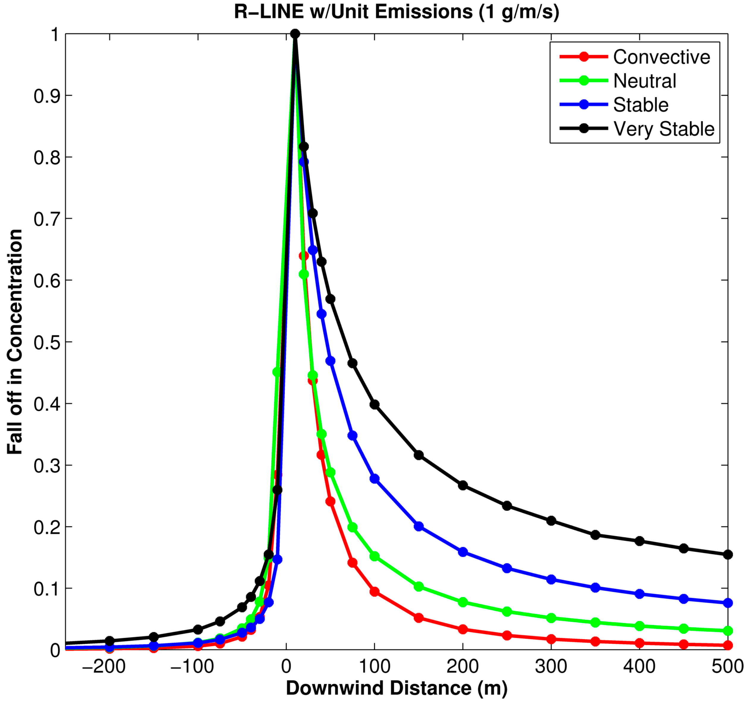
Figure 6 reflects the temporal pattern of traffic volumes used to estimate link-based emissions during the five time periods. . The AM-peak is when the highest concentrations occur for all three participant groups; this is due to the high emissions, but also the stable dispersion conditions that occur during these hours. In fact the impact of roadway emission on the low traffic cohort in the AM peak is higher than the morning off-peak, mid-day, and pm peak of the other two cohorts. This means that meteorologically stable conditions and the elevated roadway emissions impact all groups.

Figure 7, which shows the average hourly pollutant concentrations for three pollutants, indicates that the emissions are the main driver behind the mobile-source concentrations at all study participant locations. The CO median concentrations are very similar for both high-traffic cohorts, once again confirming that CO is a marker for high traffic. Also, there are slightly higher PM_2.5 average daily concentrations for the high-diesel cohort, indicating these pollutants as diesel traffic markers.

Figure 7. Average hourly pollutant concentrations for PM_2.5, CO, and NO_x for the fall 2010 period, separated into high-traffic, high-diesel (HTHD), high-traffic, low-diesel (HTLD), and low-traffic (LT) zones.

Figure 7. Average hourly pollutant concentrations for PM_2.5, CO, and NO_x for the fall 2010 period, separated into high-traffic, high-diesel (HTHD), high-traffic, low-diesel (HTLD), and low-traffic (LT) zones.

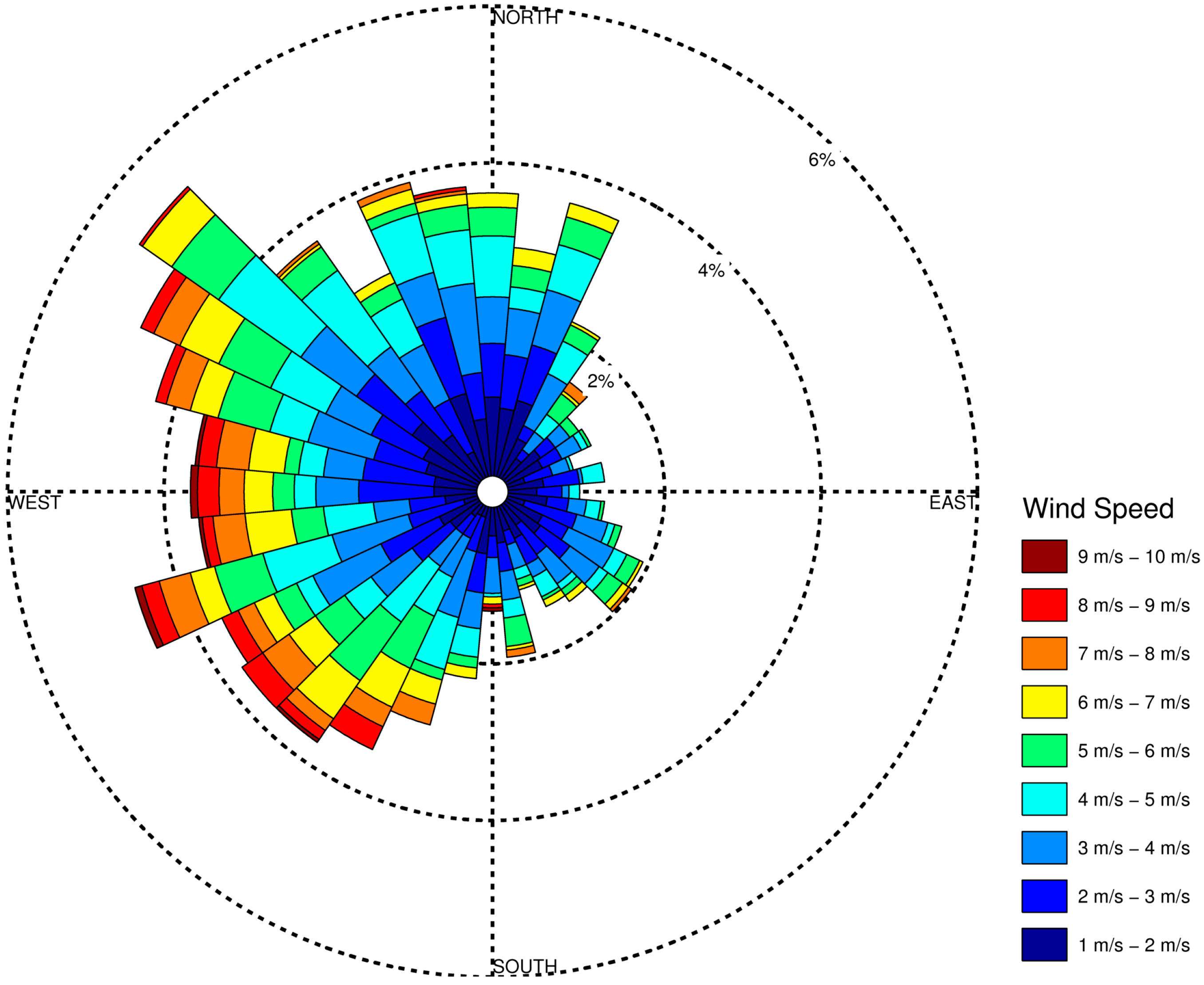
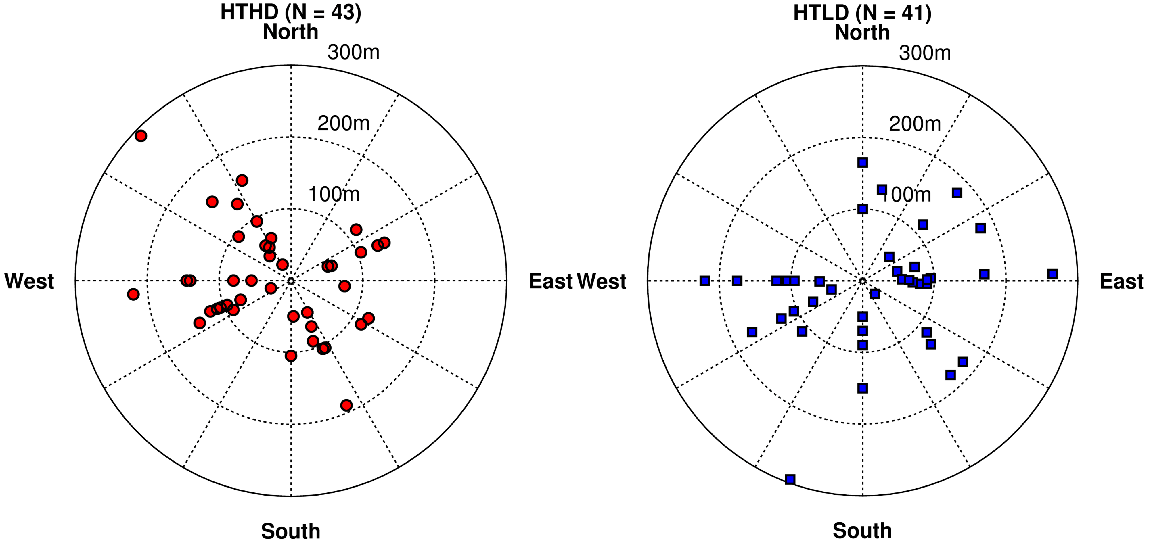
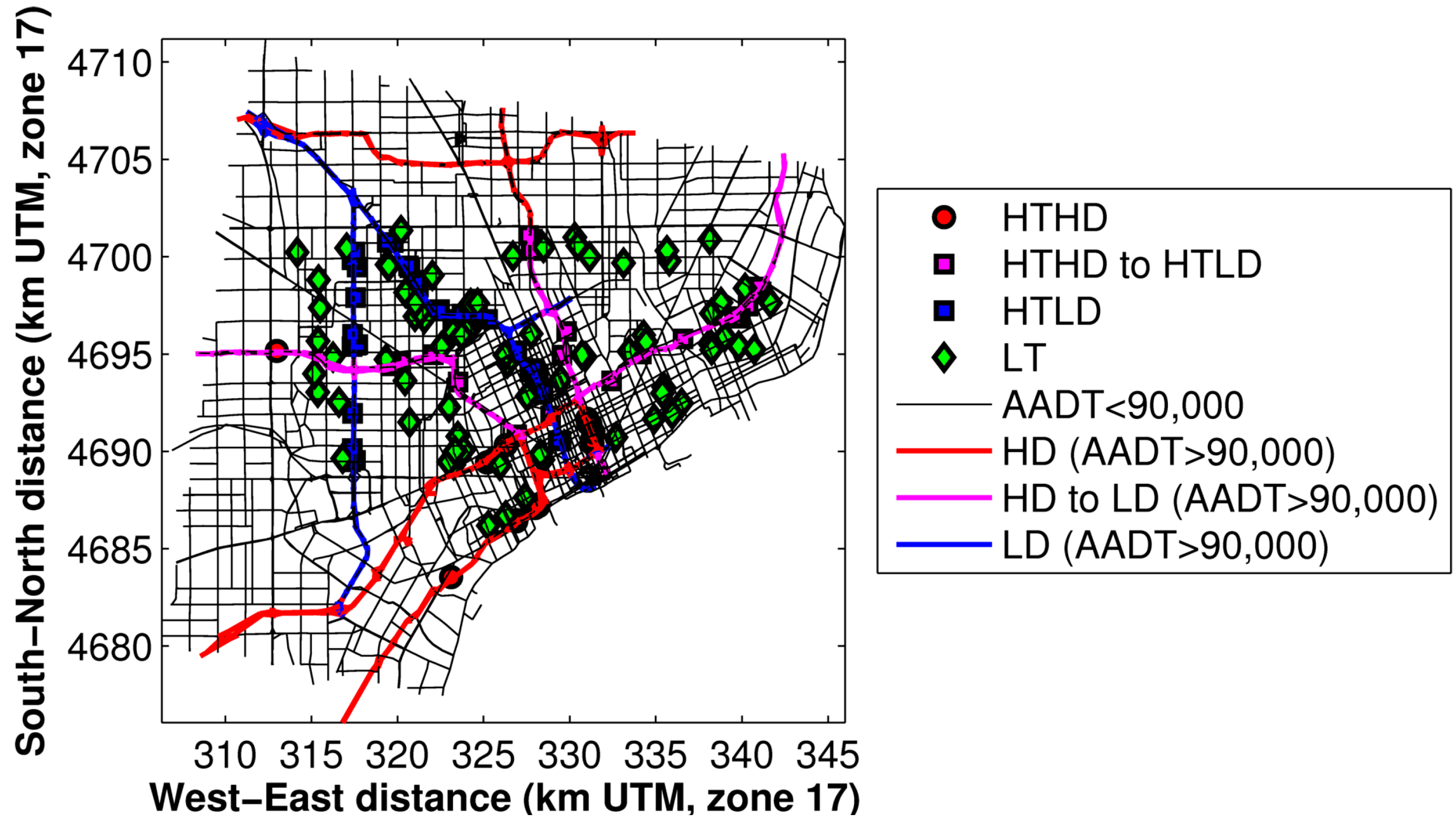
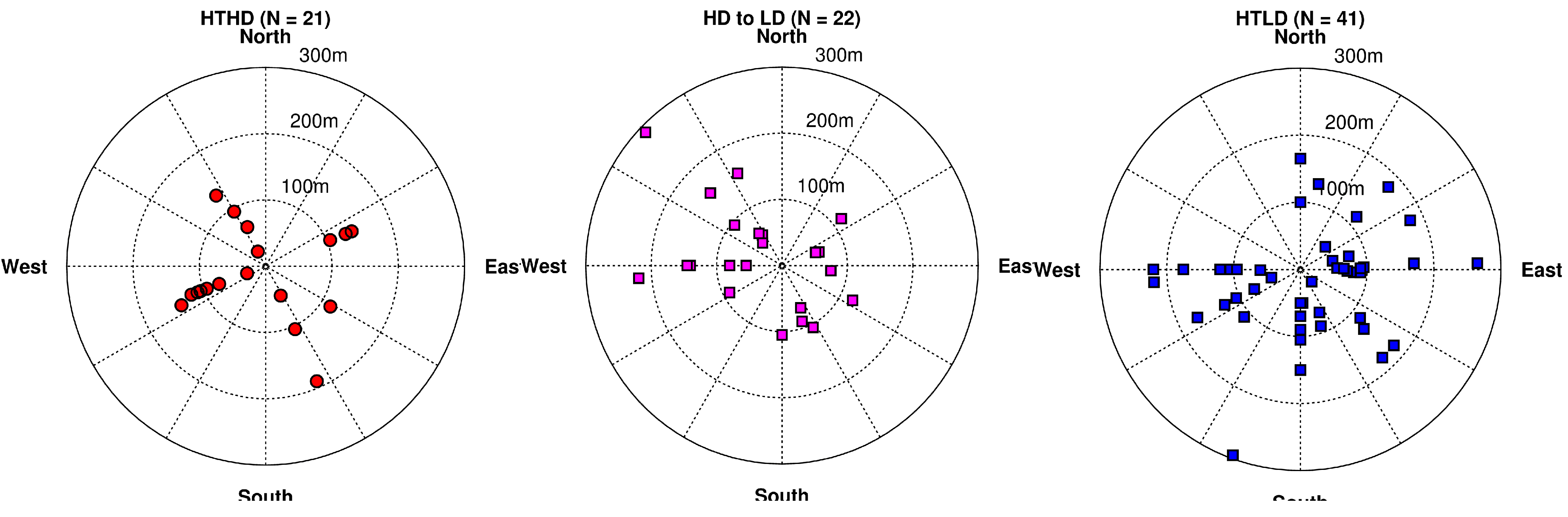
The orientation of the participants’ homes with respect to the roadway is important in analyzing results, so we examine this information in Figure 8. Examining these plots with the wind rose in Figure 4, we find that the most prevalent wind direction and a large percentage of the most stable meteorological conditions occur when the wind is blowing from the northwest toward the southeast. As a result, the participants to the southeast will have the highest exposures and participants to the northwest will have the lowest exposures. Note that some of the HTHD participants (this term refers to the cohort of participants living near high-diesel roadways) have exposures to PM_2.5 less than the HTLD participants (the cohort of participants living near lower-diesel roadways). This is due to the lack of HTLD participants in the lowest exposure wind direction quadrant, the northwest quadrant. Also, there are 39 HTHD participants within 150 m of the roadway as compared to 30 HTLD participants, which explains the distribution of CO in Figure 7 being slightly higher for the HTHD participants.

Figure 8. Locations of study participants’ homes with respect to two types of roadways: high traffic and high fraction of diesel vehicles (left panel), and high traffic and low fraction of diesel vehicles (right panel). Radial distances represent the perpendicular distance from the roadway to the study participants’ home locations.

Figure 8. Locations of study participants’ homes with respect to two types of roadways: high traffic and high fraction of diesel vehicles (left panel), and high traffic and low fraction of diesel vehicles (right panel). Radial distances represent the perpendicular distance from the roadway to the study participants’ home locations.

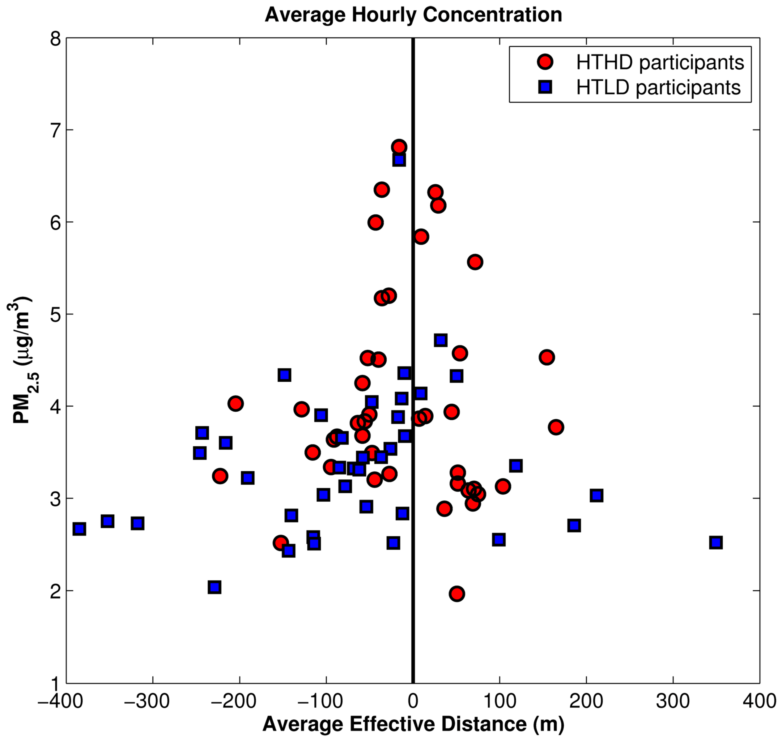
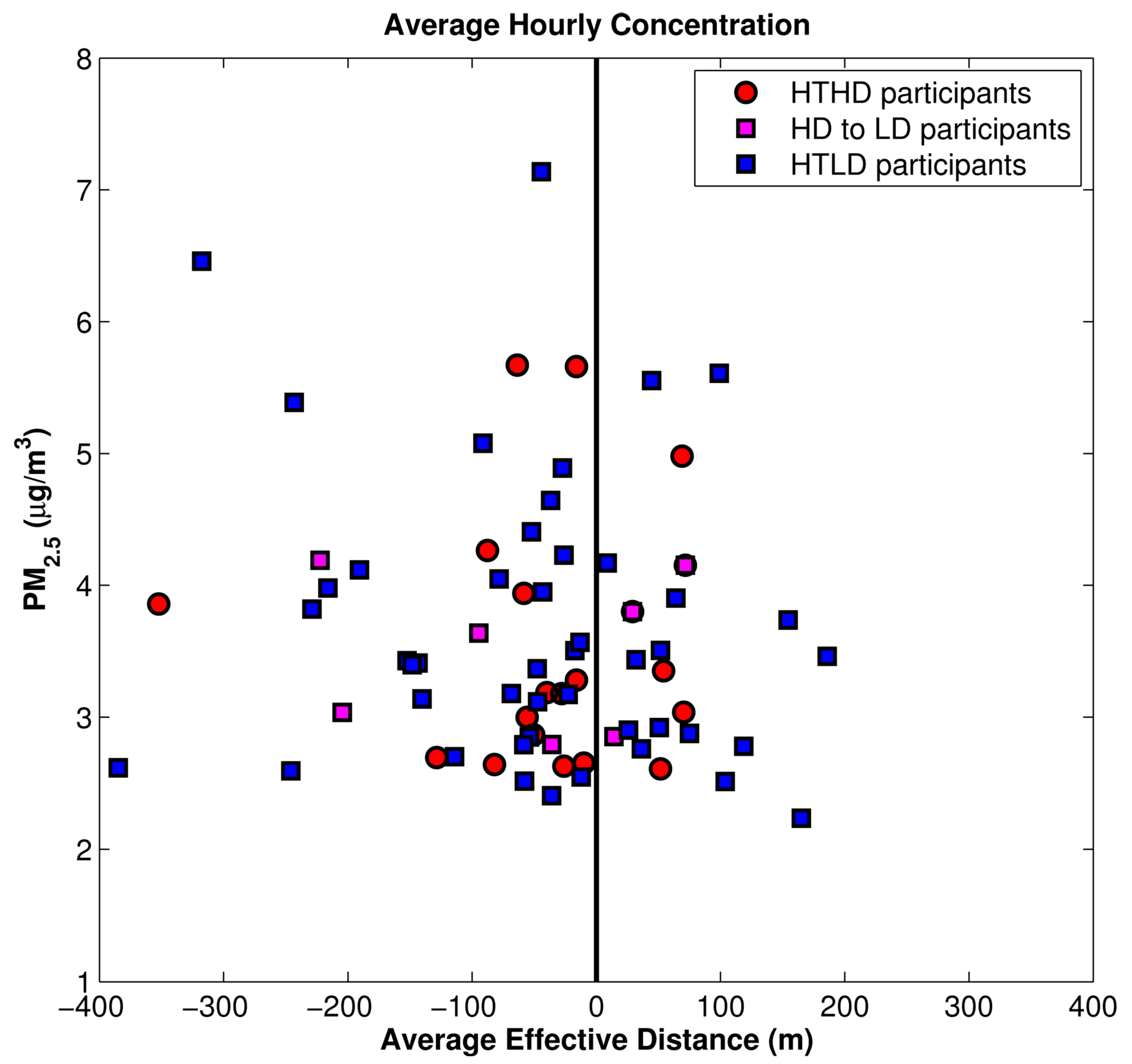
We took the analysis one step further to examine the average hourly concentration of PM_2.5 as a function of effective distance from the roadway for the two high-traffic cohorts (Figure 9). “Effective distance” utilizes hourly wind direction to compute the distance in the wind direction between the source and the receptor, and it was used with good success in an earlier health study in Detroit [19]. This figure shows a slight high bias in concentrations in the high-diesel cohort, especially when the effective distance from the roadway is very small.

Overall, the results are consistent with the NEXUS study design. The HTHD cohort has higher exposures to diesel-related pollutants, such as PM_2.5 and NO_x, than does the HTLD group. Also, both of the high-traffic cohorts have high exposures to traffic-related pollutants such as CO. This means that the methodology of combining emissions estimation and dispersion modeling is a valid tool to use for both long- and short-term health studies examining traffic-related pollutants.

Figure 9. Average hourly concentration for PM_2.5 vs. effective distance for HTHD and HTLD participants.

Figure 9. Average hourly concentration for PM_2.5 vs. effective distance for HTHD and HTLD participants.

4.2. Impacts of Adjusting Emissions Inputs Using Local-Scale Information

The methodology described in Section 2.1 uses MOVES emissions and SEMCOG roadway speeds and volumes to estimate mobile-source pollutant emissions, and our results (Section 4.1) seem to confirm the validity of the study design. However, it is important to remember that the validity of the outputs from this methodology is highly dependent on the accuracy of the inputs to the emissions modeling. We therefore decided to see whether we could improve our emissions estimates by incorporating local-scale data into our analysis.

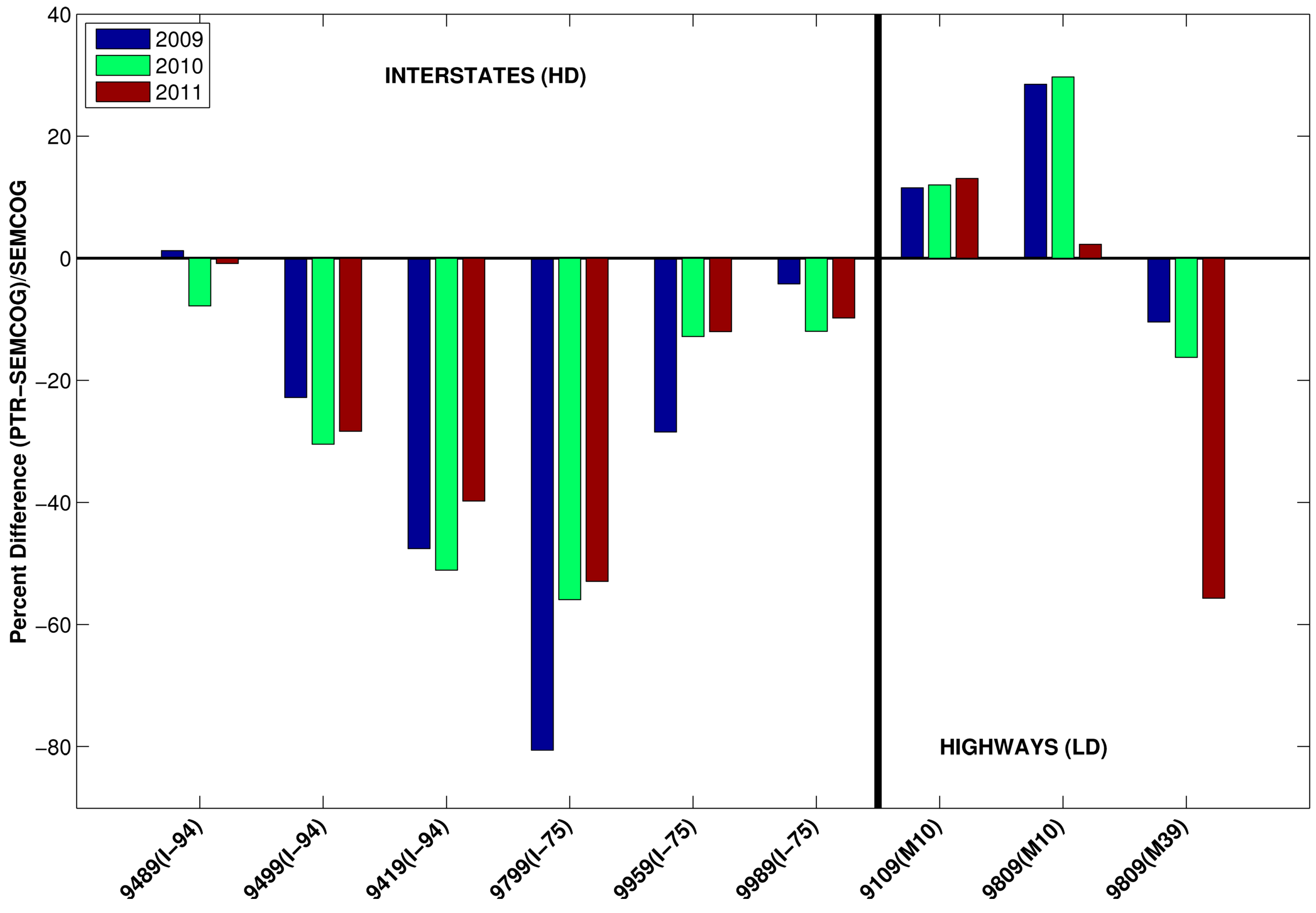
As noted earlier, the AADT (total traffic volume) estimates we used from the SEMCOG database are not based upon measurements but rather TDM outputs, calculated for all road links in the Detroit area using limited, short-term measurements, TAFs, and vehicle records. However, there is an alternative database available in which the data are local-scale measurements (although this data set does not cover all Detroit road links). The Michigan DOT (MDOT) has deployed a network of real-time permanent traffic recorders (PTRs) on many major roadways in the Detroit area [20]. To compare our SEMCOG-based results with results generated using local measurements from the PTRs, we equated PTR AADTs to TDM-based AADTs in our emissions modeling, and in cases where measurements or estimates of the commercial AADT (CAADT) were available, we equated these to diesel percentage.

We first selected links from the SEMCOG database that had corresponding real-time measurements from PTRs. Consistent with the study design, we split these links into interstates and freeways, and then compared the model-generated versus measured AADTs. Because AADT represents the average traffic for any day of the year, we took the yearly total and found the average daily vehicle count, to remove the influence of seasonal and day-of-week variations. Also, we analyzed traffic counts from 2009 and 2011 as well as 2010 to evaluate whether the differences between AADT from SEMCOG’s TDM and from the traffic counters could be attributed to an increasing or decreasing traffic volume trend or the economic struggles of the automotive industry in Detroit in 2010. The comparison is shown in Figure 10; locations of the PTR measurements are shown in the supplemental material (Figure S5).

Figure 10. Comparison of AADT from SEMCOG TDM runs versus measured AADT at selected MDOT PTR locations, shown as percent difference. This figure contains measurements at multiple locations (each group of bars); the interstates are shown on the left side of the figure and the highways are shown on the right side of the figure.

Figure 10. Comparison of AADT from SEMCOG TDM runs versus measured AADT at selected MDOT PTR locations, shown as percent difference. This figure contains measurements at multiple locations (each group of bars); the interstates are shown on the left side of the figure and the highways are shown on the right side of the figure.

First, the figure indicates that the differences for 2010 were not influenced by trends or economic conditions. Next, evaluating the estimation error in the SEMCOG TDM results by comparing them with the MDOT PTR measurements indicated that the amount of error ranged from a 45% underestimation to a 35% overestimation. This difference translates directly to a +45 to −35% uncertainty in pollutant concentration, since traffic volume is just a weighting factor in the emissions estimation. Although this range represents a significant amount of uncertainty, it is impossible to eliminate all of it without a PTR on every road link. Based on the results of Figure 10 we repeated the emissions estimations after decreasing the SEMCOG AADT on all interstates (NFC 11) by 20%, an average percent difference for the road links measured. To maintain consistent vehicle miles traveled (VMT) across the whole study domain, we made a corresponding increase of SEMCOG AADT on all freeways (NFC 12) based on the ratio of total interstate length to freeway length.

In addition to total volume measurements (AADT), MDOT also has data for commercial AADT (CAADT). This allowed us to evaluate the diesel/nondiesel percentages that we used to estimate emissions for each road link. We found that on many high-diesel (HD) interstates (NFC 11), the diesel percentage was only 5% (see Table 7), not the 9% that was previously modeled based on the aggregation of fleet mixes and local demographics.

Table 7. Comparison of diesel percentages based on NFC class and CAADT/AADT measurements on selected interstates and freeways.

Roadway Characteristic	Interstates (NFC 11)			Freeways (NFC 12)
	I-75	I-94	I-96	M10	M39
Diesel percentage in NFC class fleet mix	9%	9%	9%	5%	5%
Diesel percentage based on MDOT measurements (CAADT/AADT)	9% 5% (north of downtown)	9% 5% (east of downtown)	9% 5% (north of downtown)	5%	5%

Table 7. Comparison of diesel percentages based on NFC class and CAADT/AADT measurements on selected interstates and freeways.

Roadway Characteristic	Interstates (NFC 11)			Freeways (NFC 12)
	I-75	I-94	I-96	M10	M39
Diesel percentage in NFC class fleet mix	9%	9%	9%	5%	5%
Diesel percentage based on MDOT measurements (CAADT/AADT)	9% 5% (north of downtown)	9% 5% (east of downtown)	9% 5% (north of downtown)	5%	5%

It became clear that the use of 9% in our previous modeling had overestimated the diesel impact for study participants living near these roadways. We therefore performed an additional sensitivity simulation in which we decreased the diesel percentages on these roadways, which results in some HD roadways being reclassified as LD roadways. We also reclassified some of the study participants’ home locations, because previously they were within 300m of a HTHD roadway. Now they are within 300 m of a HTLD roadway. These combined adjustments are shown in Figure 11.

After making the adjustments in traffic volume and fleet mix analysis, we repeated the analyses discussed in Section 3.1 and shown in Figure 6, Figure 7, Figure 8 and Figure 9. The results are given in Figure 12, Figure 13, Figure 14 and Figure 15. Again, Figure 12 reflects the temporal pattern of the traffic volumes used to estimate link-based emissions. Comparing the three panels of this figure shows less distinction between the estimated concentrations for all three HT groups than was shown in Figure 6 between the two HT groups (the left and middle panels).

Reclassification of some study participants from the HD group to the LD group shown as HD to LD in Figure 13 shows that there is less distinction between the HD and LD participant groups as compared to Figure 7. The group classification was based on proximity to a HT roadway and the classification of the roadway; however the dispersion model, which produces concentrations, also takes into account the wind direction and actual distance between the roadway and the participants’ home location. We again plotted the radial distance and the wind direction normal to the roadway with HT.

Figure 11. NEXUS study domain, after making adjustments in diesel impact. Interstates (HD) and participants within 150 m of high-traffic/high-diesel (HTHD) roadways are shown in red; freeways (LD) and participants within 150 m of low-diesel/high-traffic roadways are shown in blue; control-group participants >300 m from interstates or freeways are in green; and participants and roadways that were reclassified from HD to LD are shown in magenta.

Figure 11. NEXUS study domain, after making adjustments in diesel impact. Interstates (HD) and participants within 150 m of high-traffic/high-diesel (HTHD) roadways are shown in red; freeways (LD) and participants within 150 m of low-diesel/high-traffic roadways are shown in blue; control-group participants >300 m from interstates or freeways are in green; and participants and roadways that were reclassified from HD to LD are shown in magenta.

Figure 12. Average hourly pollutant concentrations for PM_2.5 for the fall 2010 period separated into HTHD, HTLD, and LT after adjusting traffic volume and fleet mix used in the modeling. HT study participants’ whose home locations were reclassified from HD to LD are shown in magenta between the HTLD and HTLD groups.

Figure 12. Average hourly pollutant concentrations for PM_2.5 for the fall 2010 period separated into HTHD, HTLD, and LT after adjusting traffic volume and fleet mix used in the modeling. HT study participants’ whose home locations were reclassified from HD to LD are shown in magenta between the HTLD and HTLD groups.

Figure 13. Temporal distributions of mobile-source component of PM_2.5 concentration for the fall 2010 period after adjusting traffic volume and fleet mix used in the modeling. HT study participants whose home locations were reclassified from HD to LD are shown in magenta between the HTLD and HTLD groups.

Figure 13. Temporal distributions of mobile-source component of PM_2.5 concentration for the fall 2010 period after adjusting traffic volume and fleet mix used in the modeling. HT study participants whose home locations were reclassified from HD to LD are shown in magenta between the HTLD and HTLD groups.

Figure 14. Locations of study participants’ homes with respect to the roadways in the high-traffic (HT), high-diesel (HD) group (left panel); participants previously classified in the HD group who were switched to the low diesel (LD) group (middle panel); and participants in the LD group (right panel). Radial distances represent the perpendicular distance from the roadway to the study participants’ home locations.

Figure 14. Locations of study participants’ homes with respect to the roadways in the high-traffic (HT), high-diesel (HD) group (left panel); participants previously classified in the HD group who were switched to the low diesel (LD) group (middle panel); and participants in the LD group (right panel). Radial distances represent the perpendicular distance from the roadway to the study participants’ home locations.

Figure 14 shows a much smaller difference between the HD and LD participants’ exposure when compared against Figure 8. It is important to note that a significant amount of HD participants who were reclassified as LD are located to the northwest of the HT roadway. From Figure 4 the most prevalent wind direction was from northwest to southeast, where the participants living to the northwest of a roadway would have the lowest impact, this combined with the larger distance between the roadway and participants’ home leads to the on average very low impacts for the reclassified group compared to the other groups. There are still participant locations southeast of the HT roadway and most locations within 150 m of the roadway, as shown in the left panel, which will have high impacts from the HT roadway. Thus even though the HT roadways that the participant locations are adjacent to have lower emissions of some pollutants, they still have a high impact due to the orientation and proximity of the roadway near their home. Finally, we examined the average hourly concentration of PM_2.5 as a function of effective distance from the roadway, finding the average effective distance for each participant over the fall period (Figure 15).

Figure 15. Average hourly concentration for PM_2.5 vs. effective distance for HTHD participants, participants switched from HD to LD, and HTLD participants.

Figure 15. Average hourly concentration for PM_2.5 vs. effective distance for HTHD participants, participants switched from HD to LD, and HTLD participants.

The distribution of modeled PM_2.5 concentrations in Figure 15 shows that the reclassification of these roadways from HD to LD makes for less distinction between the HD and LD participants’ home locations when compared to Figure 9. In Figure 9 the HTHD participants were the majority of the locations where the highest mobile-source impact was estimated. However after the reclassification this pattern is no longer the case; the highest estimated impacts from mobile sources are shown across the HT participant locations.

In conclusion, we found that the availability of local traffic measurements should influence the overall study design, and we determined that inclusion of local measurements might alter the results concerning health outcomes when making associations between the prevalence of childhood asthma and exposure to mobile-source-related air pollutants.

5. Limitations of Methodology and Future Improvements

One of the major limitations of our methodology for modeling the impact of traffic-generated pollutants was caused by the limited amount of local road-link-specific data available in the urban area of interest. The speeds used in this modeling were obtained from a TDM model that is based on vehicle miles traveled (VMT) from local inspections, gas sales, and activity patterns between home, work, school, and amenities. This modeling probably captures overall average speeds for roadways but lacks the hour-specific data needed to capture exact hourly traffic on every road link, for direct comparison with hourly measurements. Therefore, the methodology will capture overall trends in an urban area based on meteorology, but cannot capture hourly emissions events like traffic jams or traffic detouring. Ideally, there would be measurements of AADT or traffic volume on every link in an urban area, but in reality this is not feasible.

As we conducted our extensive analysis in Detroit, we found that we were limited by the national default classifications of major roadways (either NFC 11 or NFC 12). Detroit interstates that are near study participant locations were always classified with a higher diesel percentage (NFC 11) and the major freeways with a lower diesel percentage (NFC 12). However, the availability of local measurements allowed us to reclassify stretches of interstates to lower diesel percentages. These measurements were not available when the study was originally designed, or we would have been able to select and classify participants differently. In future studies, it will be essential to conduct extensive research into the local traffic activity and roadway classifications.

We should also note that the methodology to produce link-based emissions and road link networks is very computationally expensive. On the positive side, however, this methodology is easily transferable to other applications when road network data, data on traffic patterns and speeds, and emissions factors are available.

Additionally, there are various limitations of using a dispersion model. We are able to capture only primary pollutant concentration gradients near roadways, because the chosen dispersion model does not have treatment of chemistry, and thus we cannot currently estimate the concentrations of reactive pollutants such as NO₂. We are also limited by the quality of meteorological inputs to the dispersion model. We choose DET airport meteorology as representative, but meteorological parameters could vary slightly throughout the city depending on building characteristics. Additional meteorological measurements could reduce uncertainties in the dispersion estimates, but would add a significant computational burden. That is because when multiple meteorological stations are present, dispersion from each road link would be found using meteorology from the nearest meteorological station. Additional computational burden would result from mapping roadlinks to meteorological stations and making multiple dispersion model runs, since the model is not currently setup to handle multiple meteorological station inputs. In addition, when we examined other meteorological datasets in the Detroit region, we found many contained hours with incomplete measurements, although DET was the most complete. Missing hours, especially hours that are missing certain variables in meteorological datasets, presents gaps in dispersion estimations for some sources. Thus any hour with incomplete meteorological data at any meteorological site would need to be eliminated from the analysis, leading to less data input to the health analysis and possibly weaker associations between air quality estimates and health outcomes.

6. Summary and Conclusions

We developed a bottom-up methodology for using link-based road networks and traffic activity, and used a national emissions model with local observations of hourly meteorology to develop a detailed emissions inventory. Inventory data were further used as inputs for a line-source dispersion model to estimate the effects on air quality from roadways in in support of the NEXUS study in Detroit, MI. This methodology used detailed information on roadway speeds and fleet mixes to produce highly resolved emissions estimates that vary based on roadway type and time of day.

We examined multiple aspects of the emissions and dispersion calculations used to determine pollutant concentrations at the locations of NEXUS health study participants’ homes including a multi-pollutant estimation of mobile source impacts from high-diesel and low-diesel roadways. In addition, we used local traffic measurements when available, to decrease some uncertainties in estimating traffic volume.

We also conducted a sensitivity study comparing idealized high- and low-diesel roadways, which showed that the exposure to some pollutants (e.g., PM_2.5) could differ significantly based on differences in the fleet composition of the roadway. This highlights the importance of using highly resolved roadway emissions estimates when modeling air quality near major roadways. Another key conclusion is that national or regional fleet mixes by roadway type are not always representative of the local traffic; this reinforces previous work by Lindhjem et al. [16]. Roadways classified as the same type can potentially have very different fleet mixes; thus local measurements are needed to adjust fleet mixes in order to more realistically capture exposures to pollutants from traffic, especially due to diesel fleet.

It is also important to keep in mind the broader picture. In Detroit, as in nearly all other major urban areas of the United States, there are large manufacturing/industrial sources of pollutants. The individuals that live near these facilities may be more affected by these sources than by roadways, so it is important to take into account all emissions sources when assessing the connections between exposures and adverse health effects. As part of the NEXUS study, all sources are modeled, as is the urban background air quality. The methods for obtaining the contributions of these other sources are outlined in companion papers by Isakov [6] and Arunachalam [5]. The modeled mobile-source component of air quality is important for addressing the main goals and hypotheses of the NEXUS design, but these other components should be addressed as well when forming conclusions about the overall impact of air quality on the health of study participants.