
Impacts of Climatic Variability on Vibrio parahaemolyticus Outbreaks in Taiwan


Abstract
:1. Introduction
2. Materials and Methods
2.1. Materials/Data
2.2. Methods/Analysis
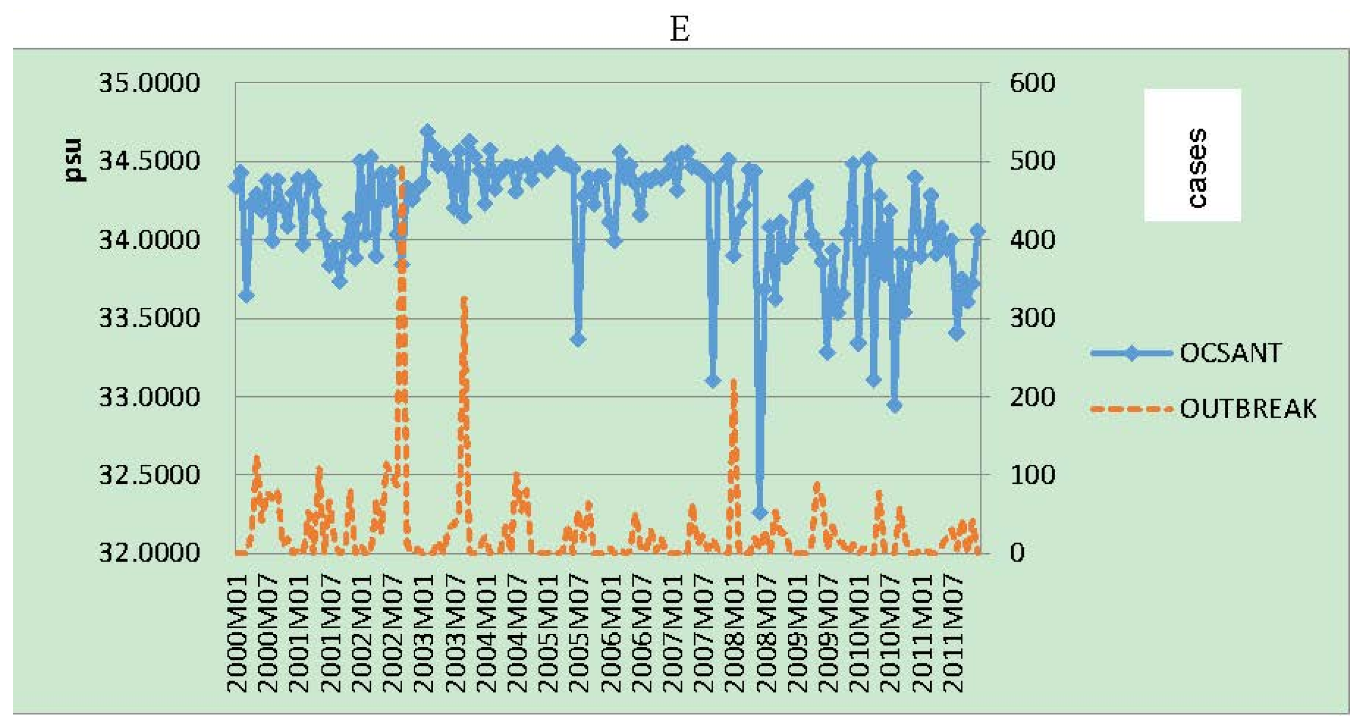
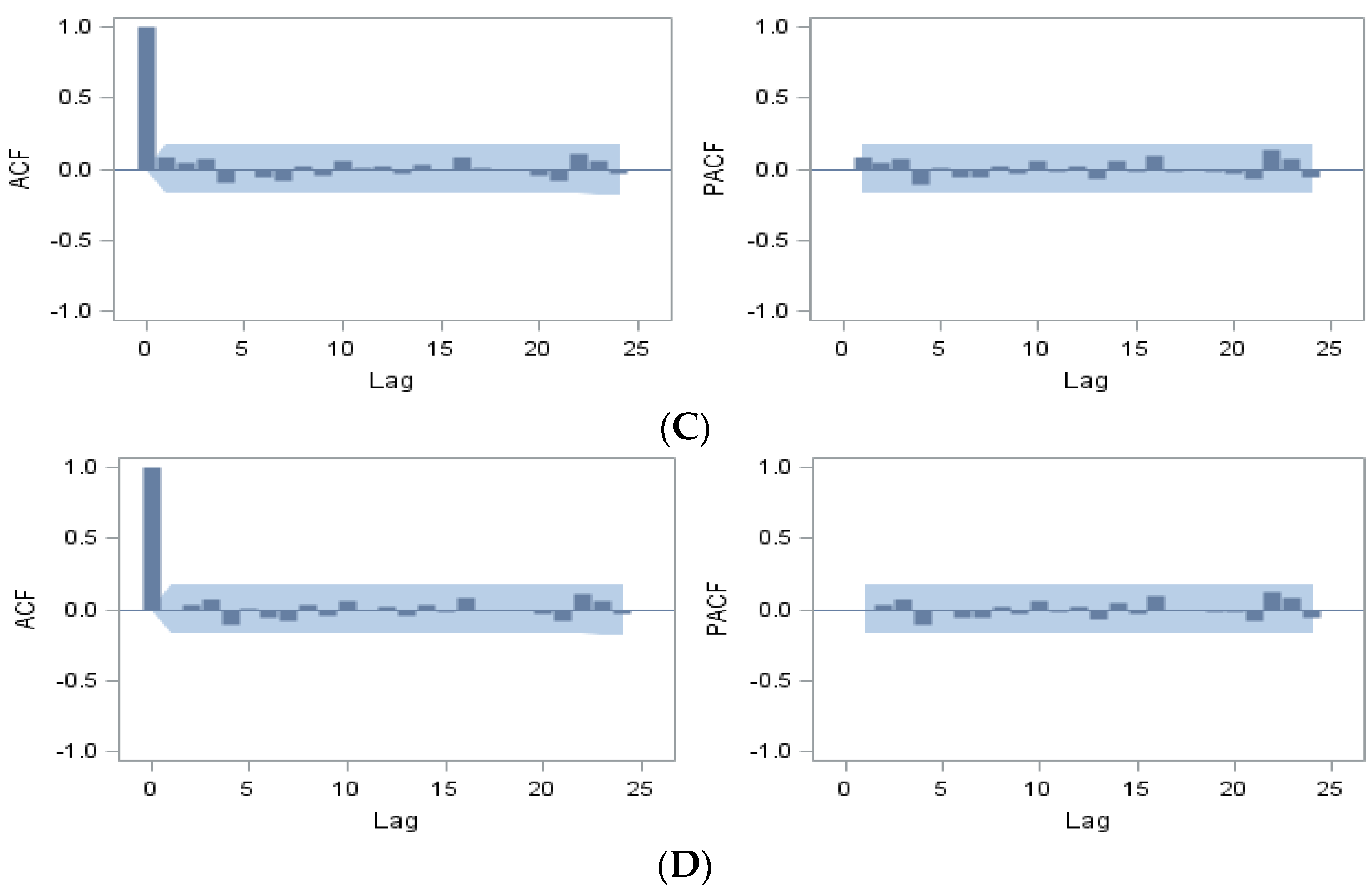
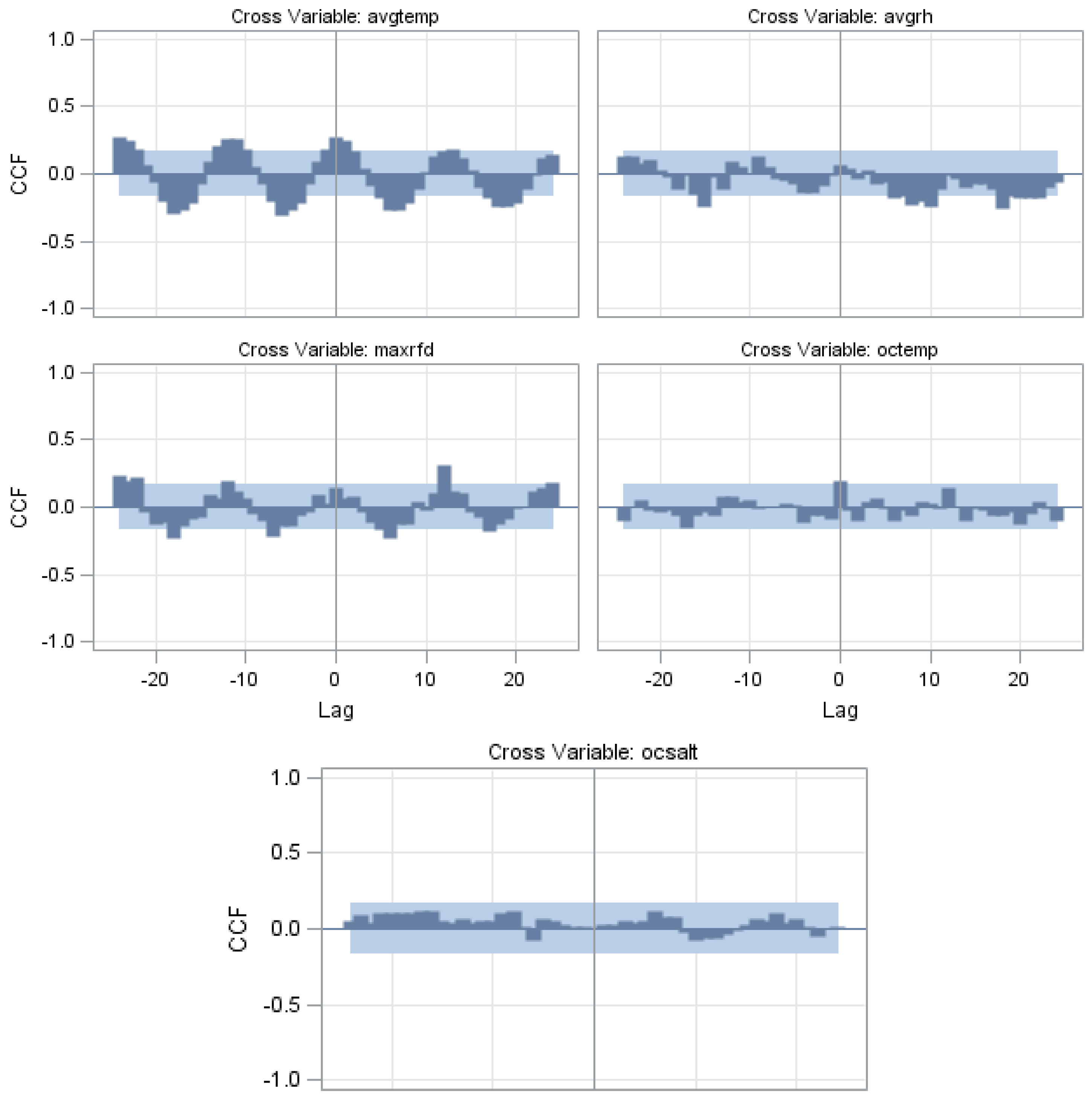
3. Results

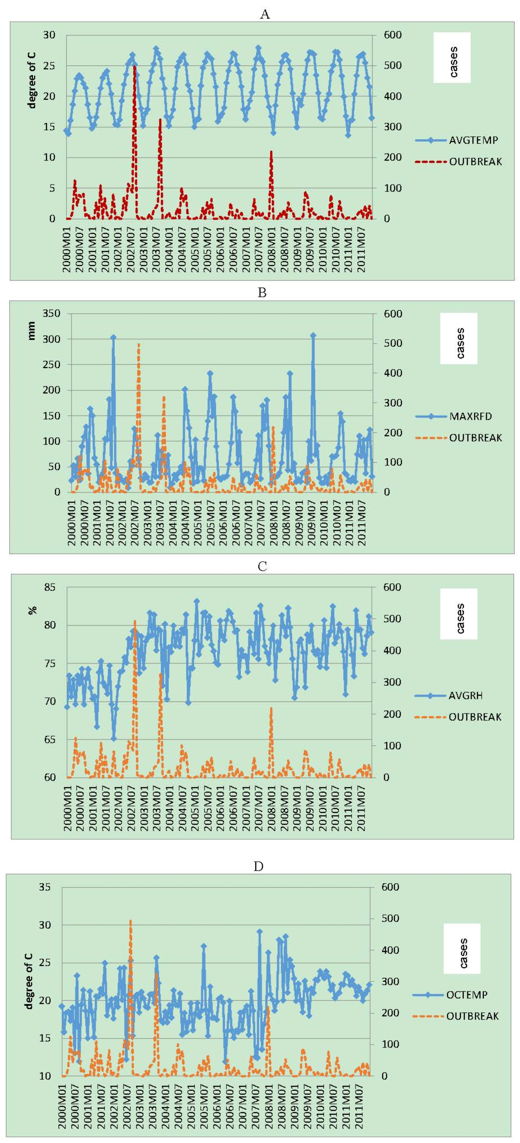
| 2000 | 2001 | 2002 | 2003 | 2004 | 2005 | 2006 | 2007 | 2008 | 2009 | 2010 | 2011 | Total | ||
|---|---|---|---|---|---|---|---|---|---|---|---|---|---|---|
| Top 5 | Pathogens | |||||||||||||
| 1 | Vibrio parahaemolyticus | 84 | 52 | 86 | 82 | 64 | 62 | 58 | 38 | 52 | 61 | 60 | 52 | 751 |
| 2 | Staphylococcus | 22 | 9 | 18 | 7 | 8 | 12 | 18 | 23 | 14 | 30 | 41 | 27 | 229 |
| 3 | Bacillus cereus | 5 | 8 | 4 | 11 | 7 | 9 | 10 | 7 | 12 | 11 | 46 | 36 | 166 |
| 4 | Salmonella | 9 | 9 | 6 | 11 | 8 | 7 | 8 | 11 | 14 | 22 | 27 | 11 | 143 |
| 5 | Pathogenic Escherichia coli | 1 | 0 | 0 | 0 | 0 | 0 | 2 | 1 | 1 | 10 | 11 | 16 | 42 |
| Top 5 | Food | |||||||||||||
| 1 | Seafood | 8 | 5 | 15 | 8 | 6 | 7 | 7 | 4 | 10 | 4 | 12 | 23 | 109 |
| 2 | Meat | 2 | 0 | 3 | 4 | 0 | 2 | 4 | 6 | 2 | 3 | 5 | 2 | 33 |
| 3 | Cereal | 2 | 2 | 2 | 0 | 0 | 5 | 7 | 5 | 2 | 2 | 1 | 4 | 32 |
| 4 | Vegetable | 1 | 2 | 1 | 1 | 8 | 2 | 2 | 1 | 0 | 0 | 5 | 7 | 30 |
| 5 | Bakery and confectionary | 3 | 3 | 0 | 0 | 2 | 0 | 1 | 0 | 2 | 4 | 4 | 1 | 20 |
| Total of food poisoning outbreaks b | 208 | 178 | 262 | 251 | 274 | 247 | 265 | 248 | 272 | 351 | 503 | 426 | 3485 |
| Variable | Avgtemp a | Maxtemp | Mintemp | Avgrf | Maxrfd | Avgrh | Maxrh | Minrh | Octemp | Ocsant |
|---|---|---|---|---|---|---|---|---|---|---|
| avgtemp | 1.0000 | |||||||||
| maxtemp | 0.9971 *** b | 1.0000 | ||||||||
| mintemp | 0.9978 *** | 0.9901 *** | 1.0000 | |||||||
| avgrf | 0.5261 *** | 0.4889 *** | 0.5516 *** | 1.0000 | ||||||
| maxrfd | 0.5577 *** | 0.5252 *** | 0.5791 *** | 0.9410 *** | 1.0000 | |||||
| avgrh | 0.4417 *** | 0.4320 *** | 0.4487 *** | 0.4498 *** | 0.3371 *** | 1.0000 | ||||
| maxrh | 0.2354 *** | 0.2590 *** | 0.2127 ** | 0.1253 | 0.0678 | 0.7315 *** | 1.0000 | |||
| minrh | 0.5781 *** | 0.5517 *** | 0.6023 *** | 0.5403 *** | 0.4856 *** | 0.7423 *** | 0.3601 *** | 1.0000 | ||
| octemp | 0.0956 | 0.1003 | 0.0913 | 0.0875 | 0.1070 | 0.1498 * | 0.1438 * | 0.0963 | 1.0000 | |
| ocsant | −0.2152 *** | −0.2096 ** | −0.2167 *** | −0.1933 ** | −0.2136 ** | −0.1204 | −0.0384 | −0.1721 | −0.4668 *** | 1.0000 |
| outbreak | 0.2675 *** | 0.2674 *** | 0.2700 *** | 0.1174 | 0.1402 * | 0.0639 | −0.0377 | 0.1273 | 0.1938 ** | −0.0064 |
| Variable (Unit) | January | February | March | April | May | June | July | August | September | October | November | December | Average | |
|---|---|---|---|---|---|---|---|---|---|---|---|---|---|---|
| outbreaks (people) | avg | 22.2 | 1.3 | 5.3 | 10.5 | 49.6 | 29.4 | 44.7 | 28.5 | 105.6 | 7.8 | 15.7 | 2.2 | 26.9 |
| max | 219 | 7 | 53 | 70 | 125 | 114 | 101 | 86 | 497 | 26 | 82 | 12 | 76.9 | |
| min | 0 | 0 | 0 | 0 | 0 | 0 | 0 | 0 | 0 | 0 | 0 | 0 | 10.4 | |
| avgtemp (°C) | avg | 15.4 | 16.5 | 17.9 | 20.9 | 23.6 | 25.2 | 26.4 | 26.3 | 25.2 | 22.9 | 20.3 | 17 | 21.4 |
| max | 16.7 | 19.4 | 19.4 | 22.2 | 24.8 | 26.4 | 27.9 | 27.2 | 26.9 | 24.4 | 21.6 | 18.3 | 22.2 | |
| min | 13.6 | 13.9 | 16.1 | 18.7 | 20.9 | 22.9 | 23.4 | 23 | 22.1 | 20.4 | 17.2 | 15.4 | 19.3 | |
| maxrfd (mm) | avg | 27.7 | 28.7 | 29.2 | 37.7 | 62.9 | 102.4 | 121.4 | 119.9 | 127.2 | 83.1 | 56.9 | 35.8 | 69.4 |
| max | 54.6 | 52.4 | 46.9 | 66.2 | 104.9 | 186.4 | 232.9 | 307.3 | 303.4 | 180.7 | 150.2 | 103.3 | 91.4 | |
| min | 17.1 | 19.2 | 17 | 8.6 | 19.4 | 37.1 | 27 | 43.5 | 36.7 | 15.2 | 17.3 | 9.2 | 46.8 | |
| avgrh (%) | avg | 75.3 | 77 | 75.4 | 76.9 | 77.3 | 79.1 | 77.2 | 78.3 | 78.1 | 75.3 | 75.5 | 73.7 | 76.6 |
| max | 80.6 | 83.1 | 79.9 | 81.6 | 81.9 | 82.5 | 80.5 | 82.5 | 82.2 | 79.7 | 81.1 | 79 | 78.8 | |
| min | 69.3 | 70.6 | 66.7 | 72.9 | 69.6 | 72.5 | 72 | 71 | 69.6 | 69.6 | 65.1 | 69 | 70.9 | |
| octemp (°C) | avg | 19.8 | 19.8 | 19.9 | 19.7 | 19.5 | 20.8 | 20 | 20.4 | 21.2 | 19.1 | 19.8 | 20 | 20.0 |
| max | 26.3 | 24.2 | 23 | 24.2 | 23.1 | 28 | 27.7 | 28.1 | 29.1 | 22.3 | 25.4 | 24.5 | 23.2 | |
| min | 15 | 15.8 | 17.1 | 15.1 | 11.9 | 16 | 12.2 | 12.4 | 11.9 | 13.5 | 15.8 | 17 | 17.2 | |
| ocsant (psu) | avg | 34.2 | 34.1 | 34.3 | 34 | 34.3 | 34.1 | 33.5 | 33.7 | 34 | 34.1 | 34.2 | 34.3 | 34.1 |
| max | 34.5 | 34.7 | 34.6 | 34.6 | 34.5 | 34.5 | 34.4 | 34.6 | 34.5 | 34.6 | 34.5 | 34.5 | 34.5 | |
| min | 33.3 | 33.1 | 33.1 | 33.1 | 33.1 | 32.3 | 27.6 | 30.6 | 33.1 | 33.5 | 33.9 | 33.9 | 32.7 | |
| Type | t-Statistic | p-Value a |
|---|---|---|
| zero mean without trend | −9.20254 | 0.0000 |
| single mean without trend | −10.8712 | 0.0000 |
| single mean with trend | −11.18945 | 0.0000 |


− 0.1734 maxrfdt-1 + 0.9559 avgrht − 4.5770 avgrht-9 + 4.5140 octempt
+13.4580 ocsantt-6 + 0.5153 εt−12 + εt


| Variable | ARIMA(1,0,0)12 a | ARIMA(0,0,1)12 | ARIMA(1,0,1)12 | ARIMA(1,0,0) × (1,0,1)12 |
|---|---|---|---|---|
| Intercept | 24.5430 *** b | 26.4550 *** | 8.4141 *** | 14.9992 |
| AR at lag1 | 0.0636 | |||
| AR at lag 12 | 0.3826 *** | 0.7526 *** | 0.7995 *** | |
| AR at lag 13 | −0.0473 | |||
| MA at lag 12 | 0.3790 *** | −0.6836 | −0.6372 *** | |
| AIC | 10.8494 | 10.8170 | 10.7066 | 10.7647 |
| RMSE | 54.0868 | 53.2847 | 49.7958 | 50.3811 |
| Variable | Covariate #1 | Covariate #2 | Covariate #3 | Covariate #4 |
|---|---|---|---|---|
| Intercept | −344.9471 | −368.2690 | −364.3913 * | −310.1019 |
| AR at lag 12 | 0.3518 *** a | −0.0211 | ||
| MA at lag 12 | 0.3230 *** | 0.5153 *** | ||
| avgtemp | 3.8521 ** | 4.7055 *** | 2.3822 | 3.5590 *** |
| avgtemp at lag1 | 2.2843 | |||
| maxrfd | −0.1022 | −0.1630 * | −0.1401 * | −0.0151 |
| maxrfd at lag1 | −0.1307 | −0.1368 * | −0.1682 ** | −0.1734 ** |
| avgrh | 1.1641 | 1.2892 | 1.2607 | 0.9559 |
| avgrh at lag9 | −4.2791 *** | −3.7936 *** | −4.0850 *** | −4.5770 *** |
| octemp | 4.7350 *** | 4.1967 *** | 4.4053 *** | 4.5140 *** |
| ocsant at lag6 | 13.0870 ** | 12.2781 ** | 12.8271 ** | 13.4580 *** |
| AIC | 10.8543 | 10.8054 | 10.7346 | 10.5413 |
| RMSE | 51.8809 | 54.5196 | 51.3805 | 48.5625 |
4. Discussion
4.1. Key Findings
4.2. Limitations
5. Conclusions
Acknowledgments
Author Contributions
Conflicts of Interest
References
- Mead, P.S.; Slutsker, L.; Dietz, V.; McCaig, L.F.; Bresee, J.S.; Shapiro, C.; Griffin, P.M.; Tauxe, R.V. Food-related illness and death in the United States. Emerg. Infect. Dis. 1999, 5, 607–625. [Google Scholar] [CrossRef] [PubMed]
- Taiwan Food and Drug Administration. Food-Borne Disease Data by Years. Available online: http://www.fda.gov.tw/TC/includes/GetFile.ashx?mID=133&id=39089&chk=8fdff827-a191-4e4b-8b81-11b876c0b7ce (accessed on 25 October 2015).
- Iwamoto, M.; Ayers, T.; Mahon, B.E.; Swerdlow, D.L. Epidemiology of seafood-associated infections in the United States. Clin. Microbiol. Rev. 2010, 23, 399–411. [Google Scholar] [CrossRef] [PubMed]
- Kirs, M.; Depaola, A.; Fyfe, R.; Jones, J.L.; Krantz, J.; van Laanen, A.; Cotton, D.; Castle, M. A survey of oysters (Crassostrea gigas) in New Zealand for Vibrio parahaemolyticus and Vibrio vulnificus. Int. J. Food Microbiol. 2011, 142, 149–153. [Google Scholar] [CrossRef] [PubMed]
- Su, Y.C.; Liu, C. Review: Vibrio parahaemolyticus: A concern of seafood safety. Food Microbiol. 2007, 24, 549–558. [Google Scholar] [CrossRef] [PubMed]
- Drake, S.L.; DePaola, A.; Jaykus, L. An overview of Vibrio vulnificus and Vibrio parahaemolyticus. Compr. Rev. Food Sci. Food Saf. 2007, 6, 120–144. [Google Scholar] [CrossRef]
- Havelaar, A.H.; Brul, S.; de Jong, A.; de Jonge, R.; Zwietering, M.H.; ter Kuile, B.H. Future challenges to microbial food safety. Int. J. Food Microbiol. 2010, 139, S79–S94. [Google Scholar] [CrossRef] [PubMed]
- Daelman, J.; Jacxsens, L.; Devlieghere, F.; Uyttendaele, M. Microbial safety and quality of various types of cooked chilled foods. Food Control 2013, 30, 510–517. [Google Scholar] [CrossRef]
- Jacxsens, L.; Kirezieva, K.; Luning, P.A.; Ingelrham, J.; Diricks, H.; Uyttendaele, M. Measuring microbial food safety output and comparing self-checking systems of food business operators in Belgium. Food Control 2015, 49, 59–69. [Google Scholar] [CrossRef]
- Van der Spiegel, M.; van der Fels-Klerx, H.J.; Marvin, H.J.P. Effects of climate change on food safety hazards in the dairy production chain. Food Res. Int. 2012, 46, 201–208. [Google Scholar] [CrossRef]
- Marques, A.; Nunes, M.L.; Moore, S.K.; Strom, M.S. Climate change and seafood safety: Human health implications. Food Res. Int. 2010, 43, 1766–1779. [Google Scholar] [CrossRef]
- Mendizabal, M.; Sepulveda, J.; Torp, P. Climate change impacts on flood events and its consequences on human in Deba River. Int. J. Environ. Res. 2014, 8, 221–230. [Google Scholar]
- Parmesan, C.; Yohe, G. A globally coherent fingerprint of climate change impacts across natural systems. Nature 2003, 421, 37–42. [Google Scholar] [CrossRef] [PubMed]
- Walther, G.R.; Post, E.; Convey, P.; Menzel, A.; Parmesan, C.; Beebee, T.J.C.; Fromentin, J.M.; Hoegh-Guldberg, O.; Bairlein, F. Ecological responses to recent climate change. Nature 2002, 416, 389–395. [Google Scholar] [CrossRef] [PubMed]
- Scavia, D.; Field, J.; Boesch, D.; Buddemeier, R.; Burkett, V.; Cayan, D.; Fogarty, M.; Harwell, M.; Howarth, R.; Mason, C.; et al. Climate change impacts on U.S. coastal and marine ecosystems. Estuaries 2002, 25, 149–164. [Google Scholar] [CrossRef]
- DaMatta, F.M.; Grandis, A.; Arenque, B.C.; Buckeridge, M.S. Impacts of climate changes on crop physiology and food quality. Food Res. Int. 2010, 43, 1814–1823. [Google Scholar] [CrossRef]
- Del Ponte, E.M.; Fernandes, J.M.C.; Pavan, W.; Baethgen, W.E. A model-based assessment of the impacts of climate variability on Fusarium Head Blight seasonal risk in Southern Brazil. J. Phytopathol. 2009, 157, 675–681. [Google Scholar] [CrossRef]
- Gouache, D.; Bensadoun, A.; Brun, F.; Pagé, C.; Makowski, D.; Wallach, D. Modelling climate change impact on Septoria Tritici Blotch (STB) in France: Accounting for climate model and disease model uncertainty. Agric. For. Meteorol. 2013, 170, 242–252. [Google Scholar] [CrossRef]
- Tirado, M.C.; Clarke, R.; Jaykus, L.A.; McQuatters-Gollop, A.; Frank, J.M. Climate change and food safety: A review. Food Res. Int. 2010, 43, 1745–1765. [Google Scholar] [CrossRef]
- Paz, S.; Bisharat, N.; Paz, E.; Kidar, O.; Cohen, D. Climate change and the emergence of Vibrio vulnificus disease in Israel. Environ. Res. 2007, 103, 390–396. [Google Scholar] [CrossRef] [PubMed]
- Chou, W.C.; Wu, J.L.; Wang, Y.C.; Huang, H.; Sung, F.C.; Chuang, C.Y. Modeling the impact of climate variability on diarrhea-associated diseases in Taiwan (1996–2007). Sci. Total Environ. 2010, 409, 43–51. [Google Scholar] [CrossRef] [PubMed]
- Kovats, R.S.; Edwards, S.; Hajat, S.; Armstrong, B.; Ebi, K.L.; Menne, B. The effect of temperature on food poisoning: A time-series analysis of salmonellosis in ten European countries. Epidemiol. Infect. 2004, 132, 443–453. [Google Scholar] [CrossRef] [PubMed]
- Fleury, M.; Charron, D.F.; Holt, J.D.; Allen, O.B.; Maarouf, A.R. A time series analysis of the relationship of ambient temperature and common bacterial enteric infections in two Canadian provinces. Int. J. Biometeorol. 2006, 50, 385–391. [Google Scholar] [CrossRef] [PubMed]
- Akin, S.-M.; Martens, P.; Huynen, M. Climate change and infectious disease risk in Western Europe: A survey of Dutch expert opinion on adaptation responses and actors. Int. J. Environ. Res. Public Health 2015, 12, 9726. [Google Scholar] [CrossRef] [PubMed]
- Davies, G.; McIver, L.; Kim, Y.; Hashizume, M.; Iddings, S.; Chan, V. Water-borne diseases and extreme weather events in Cambodia: Review of impacts and implications of climate change. Int. J. Environ. Res. Public Health 2014, 12, 191. [Google Scholar] [CrossRef] [PubMed]
- Zhang, Y.; Bi, P.; Hiller, J.E. Climate variations and Salmonella infection in Australian subtropical and tropical regions. Sci. Total Environ. 2010, 408, 524–530. [Google Scholar] [CrossRef] [PubMed]
- Tam, C.C.; Rodrigues, L.C.; O’Brien, S.J.; Hajat, S. Temperature dependence of reported Campylobacter infection in England, 1989–1999. Epidemiol. Infect. 2006, 134, 119–125. [Google Scholar] [CrossRef] [PubMed]
- Martinez-Urtaza, J.; Bowers, J.C.; Trinanes, J.; DePaola, A. Climate anomalies and the increasing risk of Vibrio parahaemolyticus and Vibrio vulnificus illnesses. Food Res. Int. 2010, 43, 1780–1790. [Google Scholar] [CrossRef]
- Box, G.E.P.; Jenkins, G.M. Time Series Analysis: Forecasting and Control; Holden-Day: Oakland, CA, USA, 1976. [Google Scholar]
- Chadsuthi, S.; Modchang, C.; Lenbury, Y.; Iamsirithaworn, S.; Triampo, W. Modeling seasonal leptospirosis transmission and its association with rainfall and temperature in Thailand using time–series and ARIMAX analyses. Asian Pac. J. Tropical Med. 2012, 5, 539–546. [Google Scholar] [CrossRef]
- MacKinnon, J.G. Numerical distribution functions for unit root and cointegration tests. J. Appl. Econom. 1996, 11, 601–618. [Google Scholar] [CrossRef]
- McLaughlin, J.B.; DePaola, A.; Bopp, C.A.; Martinek, K.A.; Napolilli, N.P.; Allison, C.G.; Murray, S.L.; Thompson, E.C.; Bird, M.M.; Middaugh, J.P. Outbreak of Vibrio parahaemolyticus gastroenteritis associated with Alaskan Oysters. New Engl. J. Med. 2005, 353, 1463–1470. [Google Scholar] [CrossRef] [PubMed]
- Parveen, S.; Hettiarachchi, K.A.; Bowers, J.C.; Jones, J.L.; Tamplin, M.L.; McKay, R.; Beatty, W.; Brohawn, K.; DaSilva, L.; DePalola, A. Seasonal distribution of total and pathogenic Vibrio parahaemolyticus in Chesapeake Bay oysters and waters. Int. J. Food Microbiol. 2008, 128, 354–361. [Google Scholar] [CrossRef] [PubMed]
- Deepanjali, A.; Kumar, H.S.; Karunasagar, I. Seasonal variation in abundance of total and pathogenic Vibrio parahaemolyticus bacteria in oysters along the southwest coast of India. Appl. Environ. Microbiol. 2005, 71, 3575–3580. [Google Scholar] [CrossRef] [PubMed]
- Lowe, J.A.; Howard, T.; Pardaens, A.; Tinker, J.; Jenkins, G.; Ridely, J.; Leake, J.; Holt, J.; Wakelin, S.; Wolk, J.; et al. UK Climate Projections Science Report: Marine and Coastal Projections. Available online: http://ukclimateprojections.metoffice.gov.uk/media.jsp?mediaid¼87905&filetype¼pdf (accessed on 20 October 2015).
- Jones, J.L. Introduction, including Vibrio parahaemolyticus, Vibrio vulnificus, and other Vibrio species. In Encyclopedia of Food Microbiology (Second Edition); Tortorello, C.A.B.L., Ed.; Academic Press: Oxford, UK, 2014; pp. 691–698. [Google Scholar]
- Borgnis, E.; Boyer, K. Salinity tolerance and competition drive distributions of native and invasive submerged aquatic vegetation in the Upper San Francisco Estuary. Estuar. Coasts 2015. [Google Scholar] [CrossRef]
- Young, I.; Gropp, K.; Fazil, A.; Smith, B.A. Knowledge synthesis to support risk assessment of climate change impacts on food and water safety: A case study of the effects of water temperature and salinity on Vibrio parahaemolyticus in raw oysters and harvest waters. Food Res. Int. 2015, 68, 86–93. [Google Scholar] [CrossRef]
- Boxall, A.B.A.; Hardy, A.; Beulke, S.; Boucard, T.; Burgin, L.; Falloon, P.D.; Haygarth, O.M.; Hutchinson, T.; Kovats, R.S.; Leonardi, G.; et al. Impacts of climate change on indirect human exposure to pathogens and chemicals from agriculture. Environ. Health Perspect. 2009, 117, 508–514. [Google Scholar] [CrossRef] [PubMed] [Green Version]
- Moore, M.V.; Pace, M.L.; Mather, J.R.; Murdoch, P.S.; Howarth, R.W.; Folt, C.L.; Chen, C.Y.; Hemond, H.F.; Flebbe, P.A.; Driscoll, C.T. Potential effects of climate change on freshwater ecosystems of the New England/mid-Atlantic region. Hydrol. Process. 1997, 11, 925–947. [Google Scholar] [CrossRef]
- Peterson, D.; Cayan, D.; Dileo, J.; Noble, M.; Dettinger, M. The role of climate in estuarine variability. Am. Sci. 1995, 83, 58–67. [Google Scholar]
- Shriner, D.S.; Street, R.B. North America. Climate change. In Contribution of Working Group II to the Fourth Assessment Report of the Intergovernmental Panel on Climate Change; Parry, M.L., Palutikof, P.J., van der Linden, C.E.H., Eds.; Cambridge University Press: Cambridge, UK, 2007. [Google Scholar]
- Chang, Y.; Lee, M.-A.; Lee, K.-T.; Shao, K.-T. Adaptation of fisheries and mariculture management to extreme oceanic environmental changes and climate variability in Taiwan. Mar. Policy 2013, 38, 476–482. [Google Scholar] [CrossRef]
- Lee, M.-A.; Yang, Y.-C.; Shen, Y.-L.; Chang, Y.; Tsai, W.-S.; Lan, K.-W.; Kuo, Y.-C. Effects of an unusual cold-water intrusion in 2008 on the catch of coastal fishing methods around Penghu Islands, Taiwan. Terr. Atmos. Ocean. Sci. 2014, 25, 107–120. [Google Scholar] [CrossRef]
- Lu, H.-J.; Lee, H.-L. Changes in the fish species composition in the coastal zones of the Kuroshio Current and China coastal current during periods of climate change: Observations from the set-net fishery (1993–2011). Fish. Res. 2014, 155, 103–113. [Google Scholar] [CrossRef]
- Mira de Orduña, R. Climate change associated effects on grape and wine quality and production. Food Res. Int. 2010, 43, 1844–1855. [Google Scholar] [CrossRef]
© 2016 by the authors; licensee MDPI, Basel, Switzerland. This article is an open access article distributed under the terms and conditions of the Creative Commons by Attribution (CC-BY) license (http://creativecommons.org/licenses/by/4.0/).
Share and Cite
Hsiao, H.-I.; Jan, M.-S.; Chi, H.-J. Impacts of Climatic Variability on Vibrio parahaemolyticus Outbreaks in Taiwan. Int. J. Environ. Res. Public Health 2016, 13, 188. https://doi.org/10.3390/ijerph13020188
Hsiao H-I, Jan M-S, Chi H-J. Impacts of Climatic Variability on Vibrio parahaemolyticus Outbreaks in Taiwan. International Journal of Environmental Research and Public Health. 2016; 13(2):188. https://doi.org/10.3390/ijerph13020188
Chicago/Turabian StyleHsiao, Hsin-I, Man-Ser Jan, and Hui-Ju Chi. 2016. "Impacts of Climatic Variability on Vibrio parahaemolyticus Outbreaks in Taiwan" International Journal of Environmental Research and Public Health 13, no. 2: 188. https://doi.org/10.3390/ijerph13020188
APA StyleHsiao, H. -I., Jan, M. -S., & Chi, H. -J. (2016). Impacts of Climatic Variability on Vibrio parahaemolyticus Outbreaks in Taiwan. International Journal of Environmental Research and Public Health, 13(2), 188. https://doi.org/10.3390/ijerph13020188