
Mapping Copper and Lead Concentrations at Abandoned Mine Areas Using Element Analysis Data from ICP–AES and Portable XRF Instruments: A Comparative Study


Abstract
:1. Introduction
2. Materials and Methods
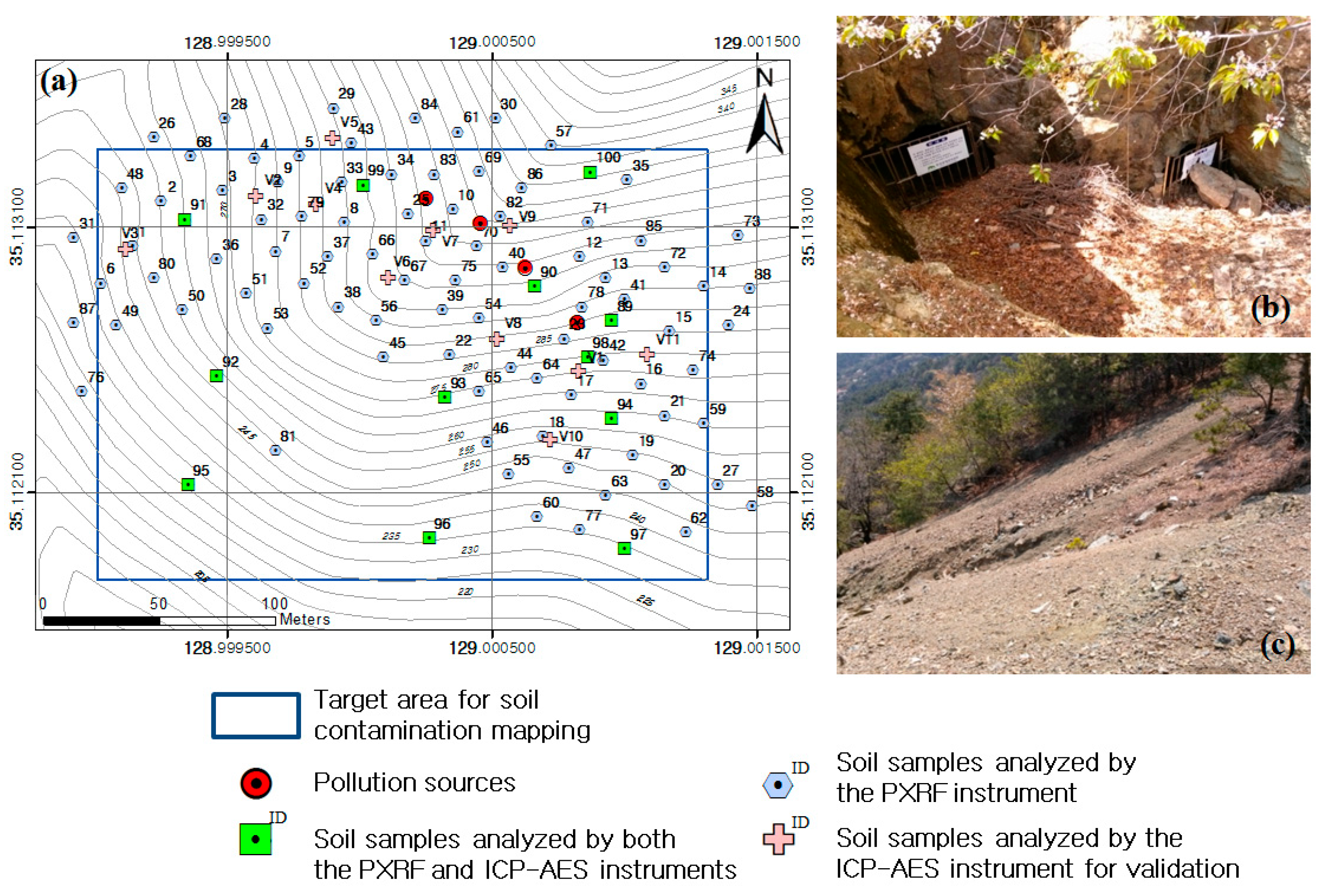
2.1. Study Area and Soil Sampling
2.2. Geostatistical Methods
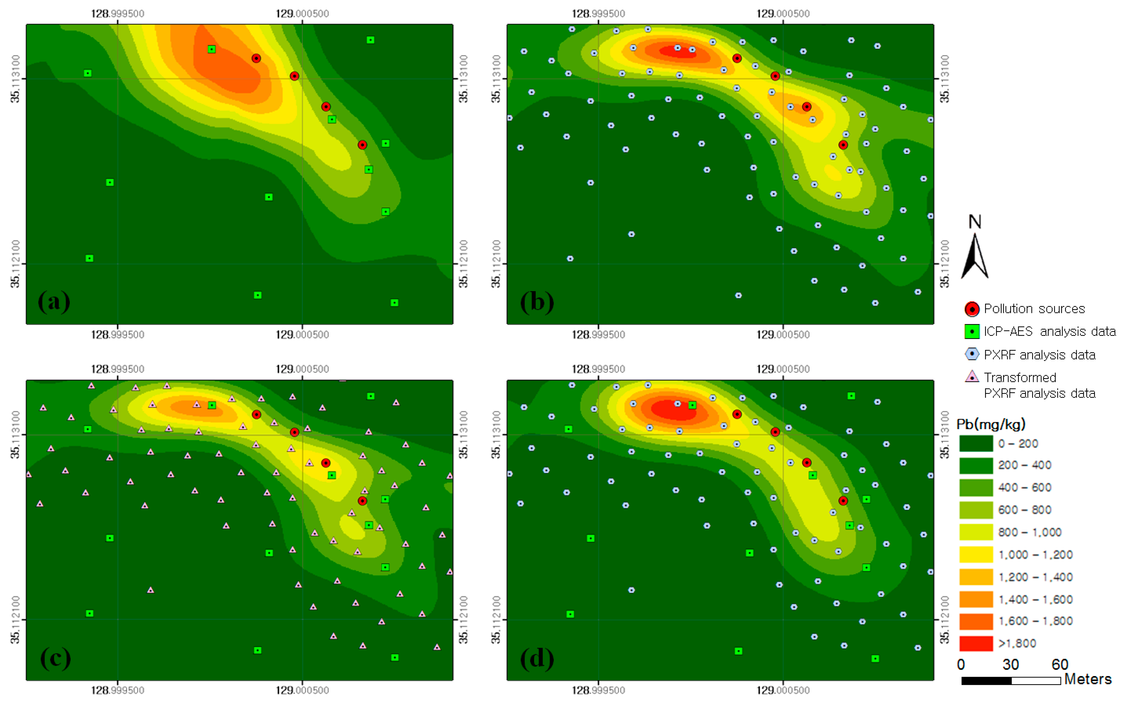
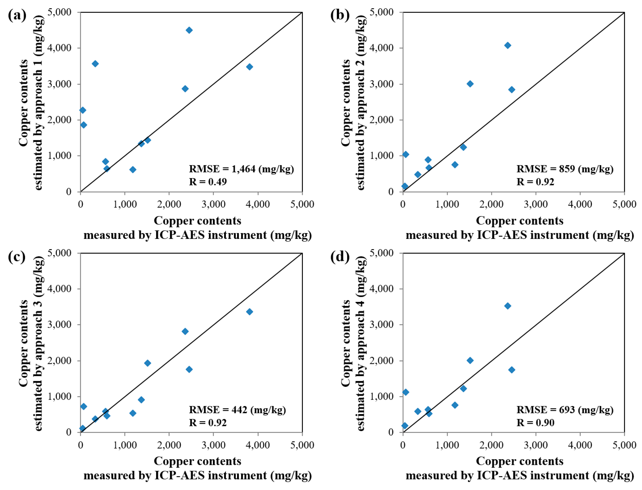
2.3. Four Different Approaches for Mapping Copper and Lead Concentrations
3. Results and Discussion
4. Conclusions
Acknowledgments
Author Contributions
Conflicts of Interest
Abbreviations
| PTEs | Potentially toxic trace elements |
| ICP–AES | Inductively coupled plasma atomic emission spectrometry |
| PXRF | Portable X-ray fluorescence |
| DEM | Digital elevation model |
| RMSE | Root-mean-square error |
References
- Kim, S.M.; Choi, Y.; Suh, J.; Oh, S.; Park, H.D.; Yoon, S.H.; Go, W.R. ArcMine: A GIS extension to support mine reclamation planning. Comput. Geosci. 2012, 46, 84–95. [Google Scholar] [CrossRef]
- Krishna, A.K.; Mohan, K.R.; Murthy, N.N.; Periasamy, V.; Bipinkumar, G.; Manohar, K.; Rao, S.S. Assessment of heavy metal contamination in soils around chromite mining areas, Nuggihalli, Karnataka, India. Environ. Earth. Sci. 2013, 70, 699–708. [Google Scholar] [CrossRef]
- Song, J.; Choi, Y.; Yoon, S.H. Analysis of photovoltaic potential at abandoned mine promotion districts in Korea. Geosyst. Eng. 2015, 18, 168–172. [Google Scholar] [CrossRef]
- Gholizadeh, A.; Borůvka, L.; Vašát, R.; Saberioon, M.; Klement, A.; Kratina, J.; Tejnecký, V.; Drábek, O. Estimation of potentially toxic elements contamination in anthropogenic soils on a brown coal mining dumpsite by reflectance spectroscopy: A case study. PLoS ONE 2015, 10. [Google Scholar] [CrossRef] [PubMed]
- Kim, S.M.; Choi, Y.; Suh, J.; Oh, S.; Park, H.D.; Yoon, S.H. Estimation of soil erosion and sediment yield from mine tailing dumps using GIS: A case study at the Samgwang mine, Korea. Geosyst. Eng. 2012, 15, 2–9. [Google Scholar] [CrossRef]
- Lee, H.; Choi, Y. A Study on the Soil Contamination Maps Using the handheld XRF and GIS in abandoned mining areas. J. Korean Assoc. Geogr. Inf. Stud. 2014, 17, 195–206. [Google Scholar] [CrossRef]
- Radu, T.; Diamond, D. Comparison of soil pollution concentrations determined using AAS and portable XRF techniques. J. Hazard. Mater. 2009, 171, 1168–1171. [Google Scholar] [CrossRef] [PubMed]
- Hou, X.; He, Y.; Jones, B.T. Recent advances in portable X-ray fluorescence spectrometry. Appl. Spectrosc. Rev. 2004, 39, 1–25. [Google Scholar] [CrossRef]
- Tolner, M.; Vaszita, E.; Gruiz, K. On-site screening and monitoring of pollution by a field-portable X-ray fluorescence measuring device. In Proceedings of the Consoil 2010 Conference, Salzburg, Austria, 22–24 September 2010.
- Higueras, P.; Oyarzun, R.; Iraizoz, J.M.; Lorenzo, S.; Esbri, J.M.; Martinez-Coronado, A. Low-cost geochemical surveys for environmental studies in developing countries: Testing a field portable XRF instrument under quasi-realistic conditions. J. Geochem. Explor. 2012, 113, 3–12. [Google Scholar] [CrossRef]
- Kalnicky, D.J.; Singhvi, R. Field portable XRF analysis of environmental samples. J. Hazard. Mater. 2001, 83, 93–122. [Google Scholar] [CrossRef]
- Carr, R.; Zhang, C.; Moles, N.; Harder, M. Identification and mapping of heavy metal pollution in soils of a sports ground in Galway City, Ireland, using a portable XRF analyser and GIS. Environ. Geochem. Health 2008, 30, 45–52. [Google Scholar] [CrossRef] [PubMed]
- Isaaks, E.H.; Srivastava, R.M. Applied Geostatistics; Oxford University Press: New York, NY, USA, 1989. [Google Scholar]
- Buttafuoco, G.; Tallarico, A.; Falcone, G. Mapping soil gas radon concentration: A comparative study of geostatistical methods. Environ. Monit. Assess. 2007, 131, 135–151. [Google Scholar] [CrossRef] [PubMed]
- Webster, R.; Oliver, M.A. Geostatistics for Environmental Scientists, 2nd ed.; Wiley: Chichester, UK, 2007. [Google Scholar]
- Buttafuoco, G.; Tallarico, A.; Falcone, G.; Guagliardi, I. A geostatistical approach for mapping and uncertainty assessment of geogenic radon gas in soil in an area of southern Italy. Environ. Earth. Sci. 2010, 61, 491–505. [Google Scholar] [CrossRef]
- Steiger, B.; Webster, R.; Schulin, R.; Lehmann, R. Mapping heavy metals in polluted soil by disjunctive kriging. Environ. Pollut. 1996, 94, 205–215. [Google Scholar] [CrossRef]
- Goovaerts, P. Geostatistics for Natural Resources Evaluation; Oxford University Press: New York, NY, USA, 1997. [Google Scholar]
- Li, X.; Lee, S.; Wong, S.; Shi, W.; Thornton, I. The study of metal contamination in urban soils of Hong Kong using a GIS-based approach. Environ. Pollut. 2004, 129, 113–124. [Google Scholar] [CrossRef] [PubMed]
- Lee, C.S.; Li, X.; Shi, W.; Cheung, S.C.; Thornton, I. Metal contamination in urban, suburban, and country park soils of Hong Kong: A study based on GIS and multivariate statistics. Sci. Total Environ. 2006, 356, 45–61. [Google Scholar] [CrossRef] [PubMed]
- Cheng, J.; Shi, Z.; Zhu, Y. Assessment and mapping of environmental quality in agricultural soils of Zhejiang Province, China. J. Environ. Sci. 2007, 19, 50–54. [Google Scholar] [CrossRef]
- Mahmoudabadi, E.; Sarmadian, F.; Savaghebi, G.H.; Alijani, Z. Accuracy assessment of geostatistical methods for zoning of heavy metals in soils of urban-industrial areas. Int. Res. J. Appl. Basic. Sci. 2012, 3, 991–999. [Google Scholar]
- MOE. Soil Contamination Assessment Report in Abandoned Metallic Mines; Ministry of Environment: Kyunggi, Gwachun, Korea, 2007; pp. 973–987. [Google Scholar]
- Buttafuoco, G.; Conforti, M.; Aucelli, P.P.C.; Robustelli, G.; Scarciglia, F. Assessing spatial uncertainty in mapping soil erodibility factor using geostatistical stochastic simulation. Environ. Earth. Sci. 2012, 66, 1111–1125. [Google Scholar] [CrossRef]
- Goovaerts, P.; Webster, R.; Dubois, J.P. Assessing the risk of soil contamination in the Swiss Jura using indicator geostatistics. Environ. Ecol. Stat. 1997, 4, 49–64. [Google Scholar] [CrossRef]
- Chile’s, J.P.; Delfiner, P. Geostatistics: Modelling Spatial Uncertainty, 2nd ed.; Wiley: New York, NY, USA, 2012. [Google Scholar]
- Roth, C. Is lognormal kriging suitable for local estimation? Math. Geol. 1998, 30, 999–1009. [Google Scholar] [CrossRef]
- Choi, Y.; Park, H.D.; Sunwoo, C. Flood and gully erosion problems at the Pasir open pit coal mine, Indonesia: A case study of the hydrology using GIS. Bull. Eng. Geol. Environ. 2008, 67, 251–258. [Google Scholar] [CrossRef]
- Choi, Y.; Yi, H.; Park, H.D. A new algorithm for grid-based hydrologic analysis by incorporating stormwater infrastructure. Comput. Geosci. 2011, 37, 1035–1044. [Google Scholar] [CrossRef]
- Choi, Y. A new algorithm to calculate weighted flow-accumulation from a DEM by considering surface and underground stormwater infrastructure. Environ. Modell. Softw. 2012, 30, 81–91. [Google Scholar] [CrossRef]


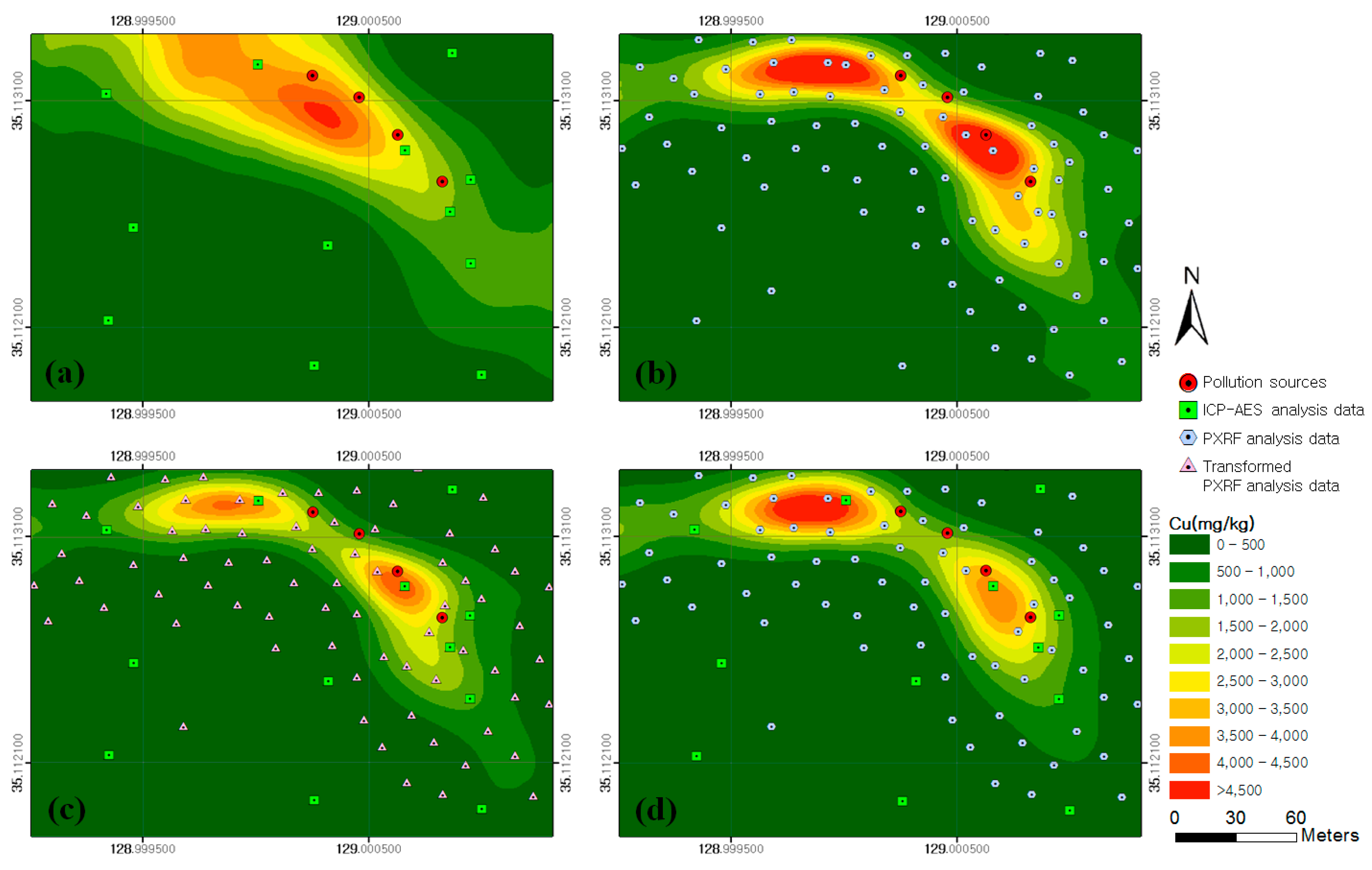
| ID | Input Data | Geostatistical Method |
|---|---|---|
| 1 | ICP–AES analysis data | Ordinary kriging |
| 2 | PXRF analysis data | Ordinary kriging |
| 3 | ICP–AES and PXRF analysis data transformed by considering the correlation between them | Ordinary kriging |
| 4 | ICP–AES (primary) and PXRF (secondary) analysis data | Co-kriging |
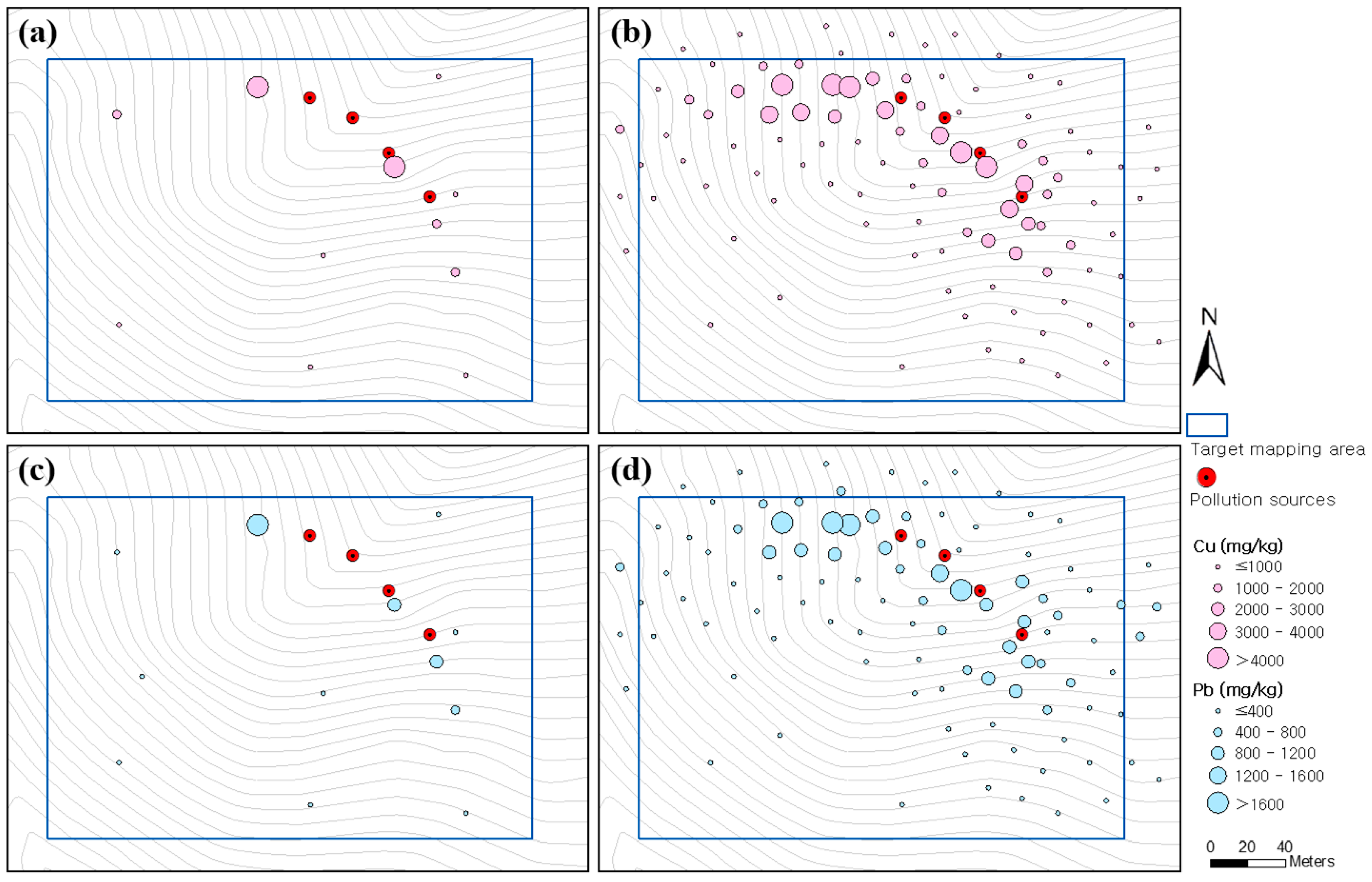
| ID | Cu (mg/kg) | Pb (mg/kg) | EC (µS·cm) | pH | Remark |
|---|---|---|---|---|---|
| 89 | 636 | 188 | 44.0 | 5.76 | 12 samples in which the PXRF and ICP–AES analyses were performed together |
| 90 | 4437 | 811 | 17.8 | 5.69 | |
| 91 | 1080 | 223 | 26.3 | 5.04 | |
| 92 | 17 | 26 | 27.1 | 4.72 | |
| 93 | 57 | 81 | 32.4 | 4.56 | |
| 94 | 1338 | 402 | 36.4 | 5.01 | |
| 95 | 33 | 59 | 51.3 | 4.80 | |
| 96 | 29 | 46 | 30.1 | 5.57 | |
| 97 | 344 | 94 | 27.6 | 4.68 | |
| 98 | 1535 | 872 | 13.7 | 5.32 | |
| 99 | 4041 | 1924 | 22.4 | 4.93 | |
| 100 | 48 | 29 | 48.3 | 5.09 | |
| V1 | 1517 | 602 | 29.7 | 4.95 | 11 samples collected at random points for validating the soil contamination maps |
| V2 | 2364 | 562 | 26.7 | 5.01 | |
| V3 | 1176 | 262 | 35.4 | 5.20 | |
| V4 | 3814 | 1545 | 30.3 | 4.95 | |
| V5 | 334 | 114 | 38.2 | 4.89 | |
| V6 | 48 | 29 | 59.6 | 4.88 | |
| V7 | 2454 | 695 | 65.0 | 4.41 | |
| V8 | 1368 | 536 | 31.7 | 5.10 | |
| V9 | 69 | 32 | 14.5 | 5.47 | |
| V10 | 589 | 132 | 37.1 | 5.21 | |
| V11 | 567 | 187 | 50.9 | 5.38 |
| ID of Approach | Element | Model | Type | Nugget | Sill | Range (Major/Minor) | Major Direction 1 | Cross-Validation | |
|---|---|---|---|---|---|---|---|---|---|
| ME 2 | RMSE 3 | ||||||||
| 1 | Cu | Gaussian model | Isotropic model | 0.6 | 3.2 | 90 | - | 475 | 2392 |
| Pb | 0.3 | 2.2 | 80 | 88 | 611 | ||||
| 2 | Cu | Geometric anisotropic model | 0.4 | 1.7 | 70/35 | 115 | 232 | 588 | |
| Pb | 0.2 | 0.8 | 75/40 | 115 | 35 | 170 | |||
| 3 | Cu | Geometric anisotropic model | 0.25 | 1.4 | 65/40 | 115 | 86 | 330 | |
| Pb | 0.2 | 0.8 | 75/40 | 115 | 29 | 140 | |||
| 4 (primary) | Cu | Isotropic model | 0.6 | 3.2 | 90 | - | 572 | 1044 | |
| Pb | 0.3 | 2.2 | 80 | 56 | 248 | ||||
| 4 (secondary) | Cu | 0.5 | 1.6 | 90 | - | - | |||
| Pb | 0.5 | 0.7 | 80 | - | - | ||||
| 4 (cross variogram) | Cu | N/A | 2.2 | 90 | - | - | |||
| Pb | N/A | 1.0 | 80 | - | - | ||||
© 2016 by the authors; licensee MDPI, Basel, Switzerland. This article is an open access article distributed under the terms and conditions of the Creative Commons by Attribution (CC-BY) license (http://creativecommons.org/licenses/by/4.0/).
Share and Cite
Lee, H.; Choi, Y.; Suh, J.; Lee, S.-H. Mapping Copper and Lead Concentrations at Abandoned Mine Areas Using Element Analysis Data from ICP–AES and Portable XRF Instruments: A Comparative Study. Int. J. Environ. Res. Public Health 2016, 13, 384. https://doi.org/10.3390/ijerph13040384
Lee H, Choi Y, Suh J, Lee S-H. Mapping Copper and Lead Concentrations at Abandoned Mine Areas Using Element Analysis Data from ICP–AES and Portable XRF Instruments: A Comparative Study. International Journal of Environmental Research and Public Health. 2016; 13(4):384. https://doi.org/10.3390/ijerph13040384
Chicago/Turabian StyleLee, Hyeongyu, Yosoon Choi, Jangwon Suh, and Seung-Ho Lee. 2016. "Mapping Copper and Lead Concentrations at Abandoned Mine Areas Using Element Analysis Data from ICP–AES and Portable XRF Instruments: A Comparative Study" International Journal of Environmental Research and Public Health 13, no. 4: 384. https://doi.org/10.3390/ijerph13040384