Abstract
The ventilation rate (VR) is a key parameter affecting indoor environmental quality (IEQ) and the energy consumption of buildings. This paper reviews the use of CO2 as a “natural” tracer gas for estimating VRs, focusing on applications in school classrooms. It provides details and guidance for the steady-state, build-up, decay and transient mass balance methods. An extension to the build-up method and an analysis of the post-exercise recovery period that can increase CO2 generation rates are presented. Measurements in four mechanically-ventilated school buildings demonstrate the methods and highlight issues affecting their applicability. VRs during the school day fell below recommended minimum levels, and VRs during evening and early morning were on the order of 0.1 h−1, reflecting shutdown of the ventilation systems. The transient mass balance method was the most flexible and advantageous method given the low air change rates and dynamic occupancy patterns observed in the classrooms. While the extension to the build-up method improved stability and consistency, the accuracy of this and the steady-state method may be limited. Decay-based methods did not reflect the VR during the school day due to heating, ventilation and air conditioning (HVAC) system shutdown. Since the number of occupants in classrooms changes over the day, the VR expressed on a per person basis (e.g., L·s−1·person−1) depends on the occupancy metric. If occupancy measurements can be obtained, then the transient mass balance method likely will provide the most consistent and accurate results among the CO2-based methods. Improved VR measurements can benefit many applications, including research examining the linkage between ventilation and health.
1. Introduction
The ventilation rate (VR) affects indoor environmental quality (IEQ) and the energy consumption of buildings. Ventilation with outdoor air is intended to remove moisture and pollutants emitted from indoor sources, and sufficiently high VRs are needed so as to not compromise IEQ and cause health, comfort, absenteeism and productivity problems [1,2,3,4,5,6,7,8,9,10]. Buildings are large contributors to energy consumption and greenhouse gas emissions, and heating, ventilation and air conditioning (HVAC) systems are the most demanding component among building energy services, accounting for an estimated 50% of building energy consumption and 20% of total energy consumption in the U.S. [11]. Excessively high VRs increase energy consumption and incur additional energy-related costs, however, the health benefits of higher VRs may greatly outweigh these costs [5]. In schools, for example, increasing the VR to be consistent with minimum recommended levels has been estimated to decrease absences related to illness and to yield a net economic benefit [6].
VRs should be consistent with minimum targets specified in building codes. Outdoor air rates specified for classrooms in ANSI/ASHRAE Standard 62.1 are the sum of personal (5 L·s−1·person−1) and area (0.6 L·s−1·m−2) minimum values [12]. Using the default occupant densities of 25 and 35 persons per 100 m2 for ages 5 to 8 and 9 and older, respectively, noted in the standard, the minimum VRs are 7.4 and 6.7 L·s−1·person−1 for the two age groups. With a ceiling height of 3 m, this is equivalent to air change rates of 2.22 and 2.01 h−1. For residential dwelling units, the same standard prescribes 2.5 L·s−1·person−1 and 0.3 L·s−1·m−2. For a 200 m2 area, 600 m3 volume, 3-bedroom dwelling with 4 occupants, the VR is equivalent to 20 L·s−1·person−1 and an air change rate of 0.48 h−1, similar to a minimum of 0.5 h−1 recommended for homes [5].
Ventilation metrics, including the VR (m3·h−1), VR per person (L·s−1·person−1), the outdoor air change rate (A, h−1) and others [13], can be determined using air flow measurements [14], pulse or constant injections of tracer gases [15,16,17,18], occupant-generated carbon dioxide (CO2) as a “natural tracer” gas [19,20,21,22,23,24,25,26], and the comparison of indoor and outdoor concentrations, concentration trends, and sometimes temperatures [27,28]. Air flow measurements from fan pressurization tests [29] provide a related measurement, the “tightness” of the building envelope. A recent review describing the use and history of air change rate measurements highlights the use of the constant tracer injection method with perfluorocarbon tracers like SF6 [13]; this method also allows multizone analyses [30]. VRs are measured for many purposes, e.g., to inform complaint-driven building investigations, to verify building system performance (e.g., commissioning), and as part of epidemiologic studies. However, obtaining accurate VR measurements can be challenging [19], and relatively few IEQ studies have adequately measured VRs or otherwise appropriately characterized the ventilation performance of buildings under study [13]. Additional information is needed to improve the understanding of the linkage between ventilation and health [31].
Occupant-generated CO2 has been widely used as a tracer gas for estimating the VR. CO2-based methods are convenient since CO2 is inert, emission sources (people) are present in all buildings and usually well dispersed throughout occupied spaces, and inexpensive and reasonably accurate measurement and logging instrumentation is available. CO2 is especially suitable for high occupancy spaces like schools since indoor levels can far exceed outdoor concentrations [32]. In addition, occupant-generated CO2 does not raise issues associated with the injection of a tracer gas, especially a potent greenhouse gas like SF6, that can concern school officials and require parental permission. CO2-based methods have been classified by the occupancy phase or the concentration trend into build-up (or “step-up” or “charge-up”), steady-state (or equilibrium), and decay (or “step-down”) phases [15,25,32]. Other CO2-based methods include pulse injections, techniques that combine multiple occupancy phases, and transient mass balance methods that can model multiple occupancy phases as well as arbitrary occupancy patterns. Guidance and standards for several of these methods is available [24,26,33]. These methods have different assumptions, strengths and limitations [24,25] and, as shown later, can produce different results.
While convenient, CO2 is not an ideal tracer gas [24]. CO2 sources are not unique, e.g., replacement air contains CO2 whether it is outside air where the global level currently averages 400 ppm, or if replacement air arises from other portions of the building. In addition, outdoor CO2 levels fluctuate daily and diurnally, e.g., levels tend to be lowest in the early afternoon and highest in the early morning with average diurnal changes from 50 to 100 ppm in large urban areas such as Baltimore, and levels vary by location, largely due to traffic-related emissions that can produce yet larger increments over the global level [34]. Also, CO2 generation rates in buildings vary over time and the time window considered for VR measurements, depending on the number of occupants and the level of metabolic activity. Generation rates are rarely measured, but instead estimated based on relationships established between occupant weight, height (or age and gender) and metabolic activity. Finally, sensor performance can be a concern. While the non-dispersive infrared (NDIR) sensors commonly used to measure CO2 are considered stable, durable and robust against interferences from other air components and pollutants, these sensors can be affected by temperature, atmospheric pressure and length of use [35].
This paper reviews and critiques CO2-based methods for estimating the VR with specific application to school classrooms. We present techniques presented in the literature, propose enhancements to the build-up method, extend the transient mass balance method, provide school grade- and age-specific emission rates needed for these methods, and discuss the effect of post-exercise recovery periods on CO2 generation. The methods are demonstrated for classrooms in four schools. Because the literature contains very few if any reports that compare CO2-based VR methods to reliable or “reference” methods for relatively large buildings like schools under real-life conditions, a difficult task but a clear gap in the literature, this review focuses on a comparison of the CO2-based methods. The paper consolidates methods and experience in the literature, and provides guidance for applications in classrooms, a critical environment with known ventilation issues.
2. Materials and Methods
2.1. Approaches to Estimating Ventilation Rates
Methods using CO2 as a tracer gas are based on a fully mixed mass balance model:
where V = room (or zone) volume (m3); C = CO2 concentration in the room (mg·m−3); CR = CO2 concentration in outdoor air or replacement air (mg·m−3); Q = flow rate of outdoor or replacement air (m3·h−1), and E = CO2 emission rate of indoor sources (mg·h−1). Generally, E is calculated as n GP, where n = number of persons in the space, and GP = CO2 generation rate per person (L·h−1), which is age- and activity level-specific (as described later). The air change rate, A (h−1), is Q/V. Concentrations throughout the zone are assumed to be equal; this should be confirmed using measurements at multiple locations [24]. This assumption can be violated by the uneven distribution of CO2 sources and by limited air distribution effectiveness. The CO2 methods discussed in this paper apply only to a single and fully mixed zone. Also, VRs derived using CO2-methods will include outdoor air delivered via both the ventilation system and infiltration. Finally, most applications of tracer gas methods assume that the VR is constant over a specific time window, i.e., the period over which the CO2 concentration trend or peak level is measured and analyzed.
The outdoor air flow rate per person, V0 (L·s−1·person−1), is obtained from air flow rate Q (m3·h−1) or A (h−1):
where the constant accounts for the volume and time conversions. If the number of occupants varies over the time when the VR is determined, then the choice of n is critical. In schools, students and staff often leave for lunch, recess and for other reasons, thus the average occupancy over the school day can be much lower than the maximum occupancy. In consequence, V0 determined using the average occupancy is higher, and often considerably (by about 50%) than that based on the maximum occupancy. To assess the adequacy of ventilation by reference to VR guidelines expressed as L·s−1·person−1, the use of the maximum occupancy appears most consistent. To understand contaminant exposures, the use of the average occupancy is preferable. This difference does not appear to have received attention in the literature, possibly because prior studies have not had continuous occupancy information, however, this issue appears important based on our recent experience in school classrooms [36].
V0 = 0.2778 A V/n = 0.2778 Q/n
VRs in both naturally- and mechanically-ventilated buildings can be affected by time-varying factors including internal heating and cooling loads, outdoor temperature and the indoor-outdoor temperature difference, and wind speed and direction [37]. In buildings using variable air volume (VAV) systems, air flow and the VR will depend on thermal load. If the VR varies in the study time window used to estimate the VR, then the assumption of a constant VR required by most of the CO2-based methods will be violated, although the VR estimate may be useful if the variation is small.
2.2. Steady-State Methods
Steady-state or equilibrium methods apply after CO2 levels have reached a steady-state concentration. The method is described by guidance and standards [16,24,33]. The steady-state air change rate, AS (h−1), is calculated as:
where n = number of persons in the space; GP = average CO2 generation rate per person (L·min−1·person−1); V = volume of the room or space (m3); CS = steady-state indoor CO2 concentration (ppm); and CR = CO2 concentration in replacement or outdoor air (ppm) (Given the widespread practice, the remainder of this paper uses concentration units of ppm). Steady-state methods assume that the CO2 generation rate (i.e., the number and physical activity of occupants) over the study time window is constant for a sufficiently long period to reach the indoor equilibrium concentration CS. (If CR changes over the time window, then the difference between CS and CR should approach a steady-state level.) ASTM [24] suggests that the measured CS should reflect at least 95% of the equilibrium value (i.e., as attained after three complete air changes), and provides comprehensive guidance for this method including methods to estimate uncertainty. As noted, steady-state methods assume the VR is constant over the study time window, and most assume that the outdoor CO2 concentration is constant.
AS = 6 × 10⁴ n GP/{V (CS – CR)}
In practice, the average age and average activity level of occupants are used to estimate Gp, the replacement air concentration CR is preferentially measured [24] or assumed to be 400 ppm [38], and CS is determined as the maximum 5- to 20-min average concentration over the study time window [1]. Some spaces may not reach steady-state conditions over the workday or study period. For this reason, the steady-state method is not recommended in schools if classes last 45 min or less and the air change is below 4 h−1 [21,25]. Many schools have much lower VRs, thus, the number of occupants must be constant for at least several hours to approach steady-state levels. If occupancy varies around the time of the peak concentration, then the method’s assumptions are not met. In classrooms, averaging the number of occupants n and the generation rate GP just prior to the observed CO2 peak may avoid anomalies if the occupancy fluctuates widely.
Steady-state methods may be used to estimate the VR per person using Equation (2) or as:
where V0,S = outdoor air flow rate per person (L·min−1·person−1), and the constant converts the generation rate from hours to seconds and concentrations CS and CR from ppm to a mixing ratio. For example, using a generation rate for a moderately active adult (1.7 MET; GP = 0.46 L·min−1·person−1 (Section 2.5), CS = 1479 ppm, and CR = 400 ppm, Equation (4) gives V0,S = 7.1 L·s−1·person−1, the minimum VR recommendation for many indoor spaces, including classrooms [12].
V0,S = (1.67 × 10⁴) GP/(CS – CR)
2.3. Decay Methods
Decay or step-down methods can be used when a space is vacated after occupancy, or if there is a stepwise decrease in occupancy [16,24]. The decay air change rate, AD (h−1), for a single (and well-mixed) zone can be estimated using two CO2 measurements:
where Δt = period between measurements (h); C0 and C1 = measured CO2 concentrations over the decay period (ppm); and CR = CO2 concentration (ppm) in replacement air or the steady-state concentration at the lower occupancy in the case of stepwise decrease in occupancy. The stability of this 2-point estimate can be checked using an upper bound estimate of AD, obtained by selecting C1 and C0 as the maximum and minimum concentrations, respectively, occurring near the nominal times specified, e.g., within ±1 h.
AD = 1/Δt ln{(C1 − CR)/(C0 − CR)}
Alternatively, a sequence of CO2 concentrations over a portion of the decay period, Ct, may be used to fit a solution to Equation (1) using regression or other means:
where t = time of the measurement (h). Equation (6) can be linearized:
where CS = the steady-state CO2 concentration. The estimated decay air change rate AD is the slope of the regression of ln(C1 − CR) against time t. The regression intercept is ln(CS − CR), thus CS is equal to exp(intercept) + CR.
Ct = (CS − CR) exp(−AD t) + CR
ln(Ct − CR) = −AD t + ln(CS − CR)
Decay methods have been used to estimate VRs in schools [21,32,39,40,41]. The decay method is simple, and the regression approach does not require knowledge of CR, CS, GP, n or even V. However, there are important caveats. First, the appropriate time window for analysis can require careful selection [39,42]. The concentration change over the period must be large relative to the variation in CR and CO2 measurement error; typically, changes of 100 ppm or more may be sufficient, but at least several hundred ppm are desirable given the performance of typical instrumentation. (Many CO2 instruments report accuracies of ±50 ppm plus 1% to 2% of readings.). Second, while CO2 decay curves often display near ideal behavior in many spaces, in rooms that utilize natural ventilation, opening windows during class breaks can overestimate VRs during classes [32]. Conversely, if windows are opened during occupancy but closed afterwards, VRs will be underestimated. Opened windows also can lead to significant variation in concentrations in the space, thereby violating the well-mixed assumption. Third, in mechanically-ventilated school buildings, while windows are rarely opened (and sometimes not openable), HVAC systems typically are shut down at the end of the school day. Because of the shut-down, decay air change rates will not apply to the occupied portion of the day. This applies to most U.S. schools where shut-down may occur immediately following the last class, e.g., as early as 14:20 (2:20 p.m.). (24-h time notation is used throughout this paper.) Fourth, VAV systems will provide less ventilation air if the thermal load diminishes after the space becomes unoccupied, which would have the effect of lowering the VR during the decay period even if the HVAC system is not shutdown. This especially applies to densely occupied spaces, including some classrooms. Fifth, in both naturally- and mechanically-ventilated buildings, VRs and/or infiltration rates will depend on the indoor-outdoor temperature difference, wind speed, heating and cooling load, and other factors that may change over time. For these reasons, the decay-based VR may not reflect conditions during the (occupied) school day, although it may provide information regarding the infiltration rate. Finally, while both the two-point and multipoint methods provide identical results under idealized circumstances, the former is more sensitive to measurement error and thus may be less accurate.
2.4. Build-Up Methods
Build-up methods use the increase in CO2 concentrations following occupancy to determine VRs with the assumptions that the CO2 generation rate and VR are constant over the study time window, and the zone is fully mixed (The assumption of a constant CO2 generation rate in classrooms is discussed in Section 2.5). Build-up methods can estimate the VR just after a building is occupied, or after a step-wise increase in occupancy. The method may be preferable to both the steady-state and decay methods since the derived VR applies to the occupied period, and since steady-state conditions are not required.
There are many approaches to solving the single zone mass balance for the build-up period. One approach calculates the build-up air change rate AB (h−1) using two sequential CO2 measurements:
where Δt = period between C0 and C1 measurements (h), CS = steady-state concentration (ppm), and C0 and C1 = CO2 concentrations measured at start and end of the observation time window, respectively (ppm). CS may be derived in several ways. A 3-point method uses a third concentration, CM, measured at the midpoint in time between the C0 and C1 measurements [25]. If the build-up curve follows the expected approach for the method’s assumptions (i.e., smooth and initially rapid increase that gradually plateaus), and if the method’s assumptions are valid, then ĈS may be estimated as:
AB = 1/Δt ln{(CS − C0)/(CS − C1)}
ĈS = (CM2 – C0 C1)/(2 CM – C0 − C1)
Appropriate times for measuring C0, C1 and CM in classrooms and other applications will depend on occupancy patterns and building system operation. Because build-up curves may not follow the expected approach due to time-varying occupancy or other reasons, Equation (9) can be sensitive to the time period selected (e.g., the estimated CS can be negative and meaningless if CM is less than the average of C0 and C1).
A second solution technique for the build-up method is proposed that circumvents some of the issues associated with the 3-point method. This uses an estimate of CS obtained by simultaneously solving Equations (3) and (8) so that AS = AB. Using the average number of occupant n (persons), age-adjusted CO2 generation rate GP (L·min−1·person−1), zone volume V (m3), replacement air concentration CR (ppm), and an initial air change rate estimate denoted as ÂB (h−1), an initial estimate of the steady-state concentration ĈS follows from Equation (3):
ĈS = 6 × 10⁴ n GP/(V ÂB) + CR
By substituting Equation (10) into Equation (8) and simplifying, ÂB can be solved for as the root of the following equation:
0 = exp(ÂB Δt) − {(6 × 10⁴ n GP/(V ÂB) + CR − C0)}/{6 × 104 n GP/(V ÂB) + CR − C1}
While no analytical solution exists, Equation (11) can be solved by numerical root-finding methods. Because Equation (11) has local minima and inflection points, a robust algorithm and an appropriate starting solution should be used. Since CS must exceed C1, ÂB is bounded and an upper bound estimate (that can be reduced slightly to use as a starting estimate) is:
ÂB,0 < 6 × 10⁴ n GP/{V C1 (1 − CR/C1)}
Equation (11) was solved using a modified Newton-Raphson method (described in Supplementary Materials). This implicit solution to the build-up method will yield results identical to the 3-point or other (exact) build-up methods under ideal circumstances. However, it may be more stable and less sensitive to the time window selected. It somewhat resembles a steady-state method encompassing a “correction factor” to account for measurements taken prior to reaching steady-state conditions [26].
A third solution method can be adopted from the ASTM E471 Standard, which includes a build-up method for a continuous injection of a tracer gas [16]. This is adopted for CO2 by subtracting CR from the series of CO2 observations measured over the study period, Ct at times t = 1 … T, expressing concentrations in ppm, and calculating the air change rate (rather than the air flow):
where T = number of measurements in the summation, i.e., the expression T−1 Σt (Ct − CR)−1 is the average of the inverse of the CO2 measurements after subtracting CR. The first term in Equation (13) is equivalent to the steady-state solution shown as Equation (3), but with the use of multiple measurements; the second term provides a “correction” given that concentrations C0 and C1, taken at the beginning and ending of the study time window, respectively, are not at steady-state. This solution to the non-steady-state problem can be sensitive to the time window selected, e.g., using the early part of the build-up curve can inflate the summation term due to relatively large values of inverse Ct, which leads to an overestimate of AB.
AB = 6 × 10⁴ n GP {Σt (Ct − CR)−1}/(V T) − Δt−1 ln{(C1 – CR)/(C0 – CR)}
A fourth solution technique for the build-up VR also uses the series of concentration measurements Ct over the build-up period with a solution to the fully mixed model
which may be linearized:
allowing AB to be obtained as the (negative) slope of ln(CS − Ct) versus time t. The regression intercept is equal to ln(CS − CR), thus, CR is estimated as CS – exp(intercept). This approach requires an estimate of CS, along with the sequence of CO2 measurements. A fifth and related solution method might use a non-linear solver to simultaneously estimate AB and CS in Equation (15), e.g., by minimizing the squared residuals.
Ct = (CS − CR) {1 − exp(−AB t)} + CR
ln(CS − Ct) = −AB t + ln(CS − CR)
Only a few applications of the build-up method in schools were identified [43,44]; these appear to have used the 3-point method (Equations (8) and (9)) to estimate CS. The build-up method may be used with relatively short occupied classroom periods and with low air change rates [32].
Build-up methods can be sensitive to the time window selected, as noted. In U.S. schools, the school day in primary and secondary schools generally starts about 07:30 to 08:00 and lasts till about 14:30 or 15:00, however, there can be considerable variation and many classrooms have substantial drops in occupancy during midday (e.g., due to lunch), in the afternoon, and at other times. In addition to sensitivity to the time window, the build-up air change rate may be more affected by incomplete mixing than the decay method [32]. The method assumes a constant CO2 generation rate, which requires that the number of occupants in the space and level of physical activity are unchanged over the time window, assumptions that are examined in Section 2.7. Finally, while the various solution techniques for the build-up method can provide identical results under idealized circumstances, the three point method requires that concentrations closely follow the expected trend; this method as well as the implicit method can be sensitive to measurement error; the implicit method also depends on the accuracy of the occupancy and emission estimates; and the ASTM method requires near-steady-state conditions to minimize errors. In contrast, the multipoint solution method using Equations (14) and (15) is potentially more robust. These issues are explored in Section 3.
2.5. Transient Mass Balance Methods
Transient mass balance methods to determine the VR use single or multiple occupancy phases, time-resolved occupancy and CO2 observations, and a numerical solution to the mass balance model, Equation (1). An approximate but useful solution is:
where Ct = observed CO2 concentration at time t (ppm); nt = sequence of occupancy rate observations at time t (persons); GP = average CO2 emission rate (L·min−1·person−1); Q = replacement air flow rate (m3·h−1), V = volume of the space (m3); CR = replacement air CO2 concentration (ppm); and Δt = time interval for CO2 and occupancy observations (h). The estimated air change rate, ATMB (h−1), is Q/V. The CO2 build-up from emission sources present in the space during the period Δt is expressed as the first exponential term, and the CO2 decay as the second term. If flow rate Q is constant, then the expression exp(−A/V Δt) in both terms is constant. Equation (16) is exact for step-wise changes in occupancy at Δt intervals (as obtained by occupant survey data). The key unknown, Q, is determined as the value that meets an error criterion, e.g., a numerical solver may be used to fit Q by minimizing the sum of squares between predicted and observed concentrations. We also recommend fitting the CO2 concentration at the beginning of the study time window using constraints, e.g., minimum of 375 ppm. Estimating this concentration, rather than selecting the CO2 measurement, will increase model fit and may avoid issues associated with an anomalous measurement, minor sensor errors, and in cases, CO2 levels above CR that remain elevated from the previous day. The term exp(−Q/V Δt), which does not change with time, may be precomputed to increase the optimization speed.
Ct + 1 = 6 × 10⁴ nt GP/Q {1 − exp(−Q/V Δt)} + (Ct − CR) exp(−Q/V Δt) + CR
The feasibility of using transient mass balance methods with CO2 to estimate VRs was shown for a university library in England in 1980 [45]; more recently, the method was used to determine outdoor air flow rates per person (V0) in 16 classrooms in nine schools (seven naturally ventilated) in England [46]. Applications of the method using tracer gases other than CO2 may be more common, e.g., the method was used with SF6 to determine VRs in 62 naturally ventilated classrooms in 27 schools in Greece; results showed strong correlation between VRs and CO2 concentrations [47]. CO2 simulations have been used to evaluate VRs in a few mechanically- and naturally-ventilated school rooms in the U.S. [22]. Smith [23] presents additional analyses, including extensions to multizone applications. Methods to estimate uncertainty using transient methods have been discussed elsewhere [23,45].
The transient mass balance method is very flexible. It does not require steady-state conditions, and it can be used with arbitrary (but known) occupancy patterns. It can estimate the VR for different portions of the day and different occupancy phases, e.g., morning, afternoon and evening periods, and include occupied and unoccupied periods, either separately or combined. (However, periods that might have different VRs should be analyzed separately.). The method has less sensitivity to the time window selected, any time interval Δt can be used, and the replacement air concentration CR can vary in time (if known). In addition, other unknown or uncertain parameters can be estimated, e.g., the replacement air concentration CR and the metabolic activity level used to determine GP (as well as the initial CO2 concentration mentioned). Such applications, however, should constrain estimated variables to ensure plausible values, aid convergence, and limit the sensitivity of results. While application-specific parameters should be used, for example, CR if estimated might be constrained to the range of 350 to 500 ppm, reflecting measurement uncertainty of ±50 ppm and an urban increment over average global levels of 50 ppm. Potentially the method can be used to account for the post-exercise recovery period that may temporally increase GP (see Section 2.5). Finally, fitting criteria can be calculated as a quality check, e.g., a minimum fraction of variance explained (R2) might be required, thus ensuring acceptable agreement between predicted and observed CO2 concentrations.
2.6. CO2 Generation Rates
The CO2-based VR methods, other than the decay method and some forms of the build-up method, require estimates of the CO2 generation rate GP, and all VR methods assume that GP is constant (or that its variation is known) over the time window used for analysis. This section uses a method documented elsewhere [24] to calculate school grade-level specific rates suitable for classroom applications. In addition, we include updated physical activity estimates and consider the post-exercise recovery period that can temporarily increase GP.
Estimates of GP can be derived using relationships established between occupant weight, height (or age and gender) and metabolic activity. The Dubois equation estimates an individual’s skin area:
where S = skin area (m2); H = height (m); and W = weight (kg) of an individual. The CO2 generation rate per person, GP (L·min−1·person−1), is the O2 consumption rate multiplied by the respiratory coefficient (0.83):
where MET = metabolic equivalent, a measure of an individual’s energy expenditure of physical activities.
S = 0.20247 H0.725 W0.425
GP = (60) (0.83) (0.00276) S MET/{(0.23) (0.83) + (0.77)}
Height and weight data of children for Equation (17) come from U.S. representative growth charts that list sex-specific data at the monthly level (Table 1) [48]. We took the 12-month average by grade level (assuming 1st grade children are between 6 and 7 years of age, 2nd grade between 7 and 8 years of age, and so on). For teachers, height and weight data for adults aged 20 to 70 years use representative U.S. statistics derived from NHANES 1999–2006 (Table 1) [49]. The relative variation in these data were calculated as the interquartile range (75th − 50th percentile) divided by the median (in percent). For height, this relative variation was 6% for both boys and girls, and 5% for adults. For weight, the relative variation was 22% and 30% for boys and girls, respectively, and 26% and 32% for men and women, respectively.

Table 1.
Height and weight data, surface area, and estimated CO2 generation rate GP by grade level (for children) and age (for adults).
Physical activity levels depend on task and intensity, and standard MET-based definitions have long been used to classify physical activity levels into sedentary (<1 to 1.5 MET), light (1.5 to <3 MET), moderate (3 to <6 MET) and vigorous (>6 MET) classifications. For youth (8–18 years of age), recent analyses suggest that resting energy expenditures exceed adult METS by about 33%, thus increasing the ranges stated; consequently, sedentary behaviors of children may range of up to 2.0 MET [50]. The recent compendium of physical activity for children most commonly lists 1.4 MET for children sitting quietly, studying, taking notes and writing, and having class discussion [51]. This value exceeds the “typical” MET levels stated in the guidance for using CO2 for ventilation evaluations, i.e., 1.0 to 1.2 MET for reading, writing and typing while seated [24]. For adults, the most recent compendium lists 1.5 MET for sitting tasks with light effort, e.g., office work, reading, computer work and talking; standing tasks with light effort, e.g., directing traffic, filing, talking and teaching physical education, range from 2.0 to 3.0 MET [52]. Again, these exceed values in the guidance noted earlier (1.0 to 1.2 MET for sitting activities noted earlier, and 1.4 and 2.0 MET for filing while standing and walking, respectively). Teachers and other adults in classrooms are expected to engage in a combination of sitting, standing and walking activities, thus a blend of sedentary and light activity levels is appropriate, e.g., 1.7 MET may be appropriate for a teacher who occasionally stands and walks about the classroom.
Using a physical activity value of 1.4 MET and averaging across boys and girls, the CO2 generation rate GP in classrooms ranges from 0.147 L·min−1·person−1 for pre-kindergarten children to 0.343 L·min−1·person−1 for 12th graders (Table 1). Several studies have used a single generation rate for 5th grade children, equivalent to 0.258 L·min−1·person−1 [1,6,8]; the strong dependence on age is important to recognize. For women, using a physical activity value of 1.7 MET and averaging across ages, GP is 0.442 L·min−1·person−1. GP estimates for adults have little sensitivity to age (<3% variation), unlike for children. The assumption of female teachers, used since most teachers (88%) in our school surveys have been women, is not significant since the total CO2 generation rate in classrooms is usually dominated by students. The total classroom emission rate can be calculated as the sum of emissions from children (grade level-specific GP multiplied by the number of students present) and adults (adult GP multiplied by the number of adults present).
The variability of the population’s height and weight can affect GP, as demonstrated using a limited sensitivity analysis. Using the relative variability described earlier and examining 6th grade children, a 6% increase in height over the nominal case (Table 1) would increase GP by 4% (average for boys and girls); 22% and 30% increases in weights of boys and girls, respectively, would increase GP by 10%, and increasing both height and weight by these amounts would increase GP by 15%. In most classrooms with a mix of children and imperfect correlation between height and weight, uncertainties due to height and weight variation are expected to be smaller. Uncertainties related to physical activity and metabolism levels, discussed below, are likely much more significant.
In most applications, the physical activity level of building occupants is unknown, and the actual value might considerably exceed the assumed level. Also, if the activity level changes, the assumption of a single and constant activity level might not adequately represent the CO2 generation rate GP. In addition, energy expenditures of occupants depend on activity levels prior to entering the space. In schools, for example, students may enter a classroom following more vigorous activity, e.g., walking/running to class, playing at recess, etc. Factors that affect the post-exercise recovery time needed to reach resting (or sedentary) metabolism levels include the duration and intensity of the preceding exercise and the individual’s condition and age, e.g., recovery periods for children are about half that of adults [53]. Information relevant to previous activity levels and the corresponding GP pertaining to students entering a classroom in the recovery period is not directly available, but can be inferred from several sources. For example, guidance for measuring the resting metabolic rate in adults in clinical settings suggests a minimum rest period of 10 to 20 min, and an abstention period of 2 h following moderate aerobic or anaerobic exercise [54]. The duration of excess post-exercise oxygen consumption (EPOC) for short and low intensity exercise across a number of studies examining adults listed in a comprehensive review of EPOC studies ranged between 6 and 30 min [55]. Comparable EPOC studies for healthy children engaged in low intensity exercise relevant for schools were not identified.
To evaluate effects of prior physical activity, we analyzed several scenarios that considered children exercising just prior to entering a classroom. For exercise, we assumed walking with light to hard effort, equivalent to 2.9 to 4.6 MET [51], and a nominal value of 3.5 MET. For recovery periods, we assumed a recovery time tREC (h) from 0.1 to 0.5 h, and a nominal period of 0.25 h (only adult values were available). The literature often represents recovery trajectories as a first-order (exponential decay) trend, but recovery durations have been reported using different methods. We assumed that the reported recovery time reached the resting metabolism rate within 5% of the pre-exercise value, and thus the recovery time rate constant KREC (h−1) = ln(0.05)/tREC (Larger percentages, 10% and 15%, were are also tested). With these assumptions, an individual’s instantaneous activity level after entering a classroom, METt, will exponentially decline to the sedentary level, METSED:
where METEXER = physical activity level during exercise (MET); and t = time elapsed since entering the classroom and the cessation of exercise (h). To gauge the importance of the recovery effect over the CO2 monitoring time window, METt is averaged over the time period the student is in the classroom and compared to METSED (assumed to be 1.4 MET), and expressed as a relative bias (%). This represents the amount of additional activity resulting from the post-exercise recovery period, and also the extent to which CO2 emissions will be underestimated if the post-exercise recovery effect is ignored.
METt = (METEXER – METSED) exp(−KREC t) + METSED
2.7. Application
Four classrooms in different primary schools were selected to demonstrate the VR methods, several of which have not been applied previous in schools, and to show a range of ventilation and occupancy conditions. The selected schools are a subset of those in a larger (Environmental Quality and Learning in Schools or EQUALS) study. These schools were located in the U.S. Midwestern states of Michigan, Illinois, Ohio and Indiana; all are mechanically-ventilated, and all were constructed or fully renovated in the past 15 years. Schools were visited and monitored in winter during the heating season (November 2015 to February 2016) when window or door opening was at a minimum. Our technicians conducted walk-through surveys of each classroom, ventilation system, school building, and grounds. Classroom dimensions were obtained using a laser tape measure. HVAC information, including system type, configuration, design and minimum air flow rates, were obtained from HVAC drawings, schedules and photos, as well as manufacturer’s specifications; this information was used to calculate VRs for comparison with those determined using the CO2-based methods. The studied spaces are summarized in Table 2.
Table 2.
Summary of tested classrooms, schools, ventilation systems and prevailing weather conditions. Local (airport) temperature and wind speed (mean and range in parentheses) for school day (08:00–15:00) and evening and morning period (18:00–06:00).
CO2 concentrations in each classroom were measured at a central location away from windows and doors using NDIR sensors (C7632A, Honeywell Corp., Morristown, NJ, USA); similar instrumentation on the school grounds or rooftop measured outdoor CO2 concentrations. CO2 data were reduced to 15 min averages. CO2 sensors were calibrated quarterly using zero air and a certified standard. Drift per season was typically below 25 ppm. Teachers in the selected classrooms were asked to maintain an occupancy log by recording the number of adults and children present every 15 min. This information was used to estimate CO2 generation rates on a 15 min basis using metabolic activity levels of 1.4 and 1.7 MET for children and adults, respectively, and the generation rates in Table 1. The effect of post-exercise recovery was not modeled, although a sensitivity analysis is performed in Section 3.3. One day with full data in each school was selected for analysis. To calculate build-up, steady-state and decay air change rates, study days were separated into several periods (see below) in which the VR was assumed to be constant. The 06:00 to 08:00 and 15:00 to 18:00 periods were excluded since the ventilation systems were turned on and off during these periods, which would change the VR. In addition, during these periods, occupancy rates changed dramatically, and the collected occupancy data may have been incomplete.
Steady-state VRs were calculated using Equation (3), the maximum 15-min CO2 concentration over the school day (08:00 to 15:00), the measured room volume, the average generation rate over the 2 h prior to the time of the maximum CO2 concentration (determined from the 15-min average data), and 400 ppm for the measured outdoor CO2 concentration, which was confirmed using the outdoor measurements. V0,S was calculated using Equation (4), the average per person CO2 generation rate in the classroom, and the number of persons in the classroom in the 2 h period just prior to the peak CO2 concentration. We determined the sensitivity to the time period and outdoor air concentration.
Decay air change rates were estimated using Equation (5), 15-min average CO2 measurements measured at 18:00 and 24:00 for the “evening” period, and concentrations at 24:00 and 06:00 for the “early morning” period. We searched for the maximum and minimum concentrations occurring within ±1 h of the nominal period, which were used as C0 and C1 in Equation (5). Comparable decay air change rates were found using regression to fit Equation (7) (results not shown). In addition, transient mass balance air change rates were estimated for the same periods using the sequence of 15 min average CO2 measurements.
Build-up air change rates were determined using the 2-point method in Equation (8) with an implicit estimate of CS determined using Equations (10) and (11), C0 and C1 measured as 15-min averages, a starting estimate given as 0.9999 × ÂB,0 from Equation (12), and the Newton-Raphson search method, described earlier (also see Supplemental Information). Given the occupancy patterns noted, we selected a nominal period from 08:00 to 12:00, but allowed actual start and end times to vary by ±1 h (as described earlier). The average CO2 generation rate over the selected time window was used to estimate CS. The build-up method was also implemented using the 3-point and ASTM methods (Equations (8), (9) and (13), respectively), the same selected times, and the 15-min concentration at the midpoint time (or the average of two consecutive 15-min concentrations given an even number of observations between C0 and C1).
Transient mass balance air change rates were determined using Equation (16) for three periods: the school day (8:00 to 15:00 p.m.), an evening period (18:00 to 24:00), and an early morning period 24:00 to 06:00). We used an interval of 15 min (Δt = 15 min) for observed and simulated CO2 concentrations, and the CO2 generation rate (using teacher-reported occupancy data). In addition to ATMB, we estimated the replacement air concentration (CR) with constraints (375 ppm < CR < 450 ppm), the children’s metabolic equivalent level within constraints (1.2 < MET < 1.6), and the CO2 concentration at the beginning of the simulation period with a constraint (C > 375 ppm). A generalized reduced gradient solver using central derivatives estimated these unknown parameters by minimizing the sum of squares between observed and simulated CO2 concentrations. VRs were estimated separately for each period. Each problem used the same initial solution. We also tested the sensitivity of results to the start and stop times and other parameters. Lastly, V0 is reported using both the average and the maximum number of occupants, and the estimated VR.
Outdoor temperatures and wind speeds measured at the airport nearest each school are shown in Table 2. During the school day (08:00–15:00), average temperatures varied considerably (−11 to 13 °C), depending on the day studied. Several days had moderately high wind speeds (up to 9 m/s for the school day average).
3. Results and Discussion
3.1. Comparison of Classrooms
Traces of observed and simulated CO2 levels over a 24-h period in the four classrooms are shown in Figure 1, and VRs determined using the four methods are listed in Table 3. Except where noted, predicted (using the transient mass balance method) and observed CO2 levels matched closely (R2 > 0.94). Results for the four classrooms are discussed in turn.
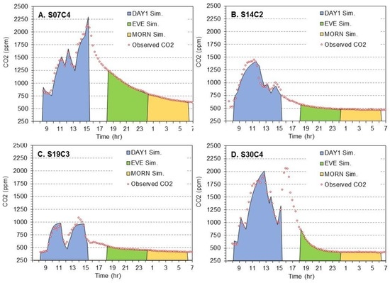
Figure 1.
Observed and simulated CO2 concentration trends over 24-h periods in classrooms in two conventional school buildings (A,B) and two EnergyStar school buildings (C,D). Red circles show observed (15-min) levels; colored areas show predicted CO2 levels using simulated air change rate estimates fitted for the school day (blue), evening (green), and early morning (yellow) periods. Time axis shows hour of day (starting at 07:00).
Table 3.
Estimated air change rates (h−1) in four classrooms based on transient mass balance, steady-state, build-up and decay methods.
Figure 1A shows trends for room S07C4. During the study period, the room contained as many as three adults and 41 children. Children were present continuously from 9:30 to 15:00 except for the lunch period (12:00 to 13:00), but the number of occupants fluctuated considerably, and the maximum occupancy occurred at the end of the school day when students from another class briefly joined the room (doubling the number of students). The “pointed” peak at the maximum CO2 concentration reveals that a steady-state level was not reached. During the school day (08:00 to 15:00), CO2 levels (15-min average) reached 2100 ppm, the transient mass balance air change rate was 0.51 h−1, the “steady-state” rate using the observed maximum CO2 level was 0.52 h−1, and build-up rates were 0.31, 0.43 and 0.52 h−1 for the 3-point, implicit and ASTM methods, respectively. All VRs calculated using CO2 fell well below those based on the HVAC schedule (shown in Table 2). Air change rates dropped to 0.14 h−1 in the evening (18:00 to 24:00) and then to 0.10 h−1 in the early morning (24:00 to 06:00). In the unoccupied period, CO2 trends followed the expected exponential decay, and the decay and transient mass balance methods gave comparable results. Based on the latter, V0 was 2.6 L·s−1·person−1 using the average occupancy (16.5 persons), but only 0.99 L·s−1·person−1 using the maximum occupancy (43 persons), an unusually large difference resulting from the large change in occupancy. CO2 levels remained above outdoor levels through the night and the next morning, a result of the previous day’s high CO2 levels and the low VR when the building was unoccupied and the HVAC system shutdown.
Figure 1B shows results for S14C2. The teacher in this classroom often shut-off the UV (the only mechanical system in the room) due to noise and opened an outside door for ventilation. This classroom contained one adult and up to 20 children. The room was continuously occupied from 07:30 to 11:45, emptied for a 45 min lunch period, and then reoccupied for two smaller classes (with a gap in between) in the afternoon. During the school day, CO2 levels reached 1440 ppm, the transient mass balance and 3-point build-up VR estimates were both 0.77 h−1; the steady state and other build-up VR estimates were lower (Table 2). V0 was 5.5 L·s−1·person−1 using the average occupancy (12.6 persons) and 3.1 L·s−1·person−1 using the maximum occupancy (22 persons). During the (unoccupied) evening and early morning periods, VRs dropped 5- to 10-fold, and the transient mass balance and decay air change rates matched closely, although CO2 levels in the early morning had only small changes, which increased uncertainty and decreased fit (e.g., R2 = 0.82). Like Figure 1A, CO2 levels the following morning remained (slightly) elevated over outdoor levels, a result of a particularly low VR during this period.
Figure 1C displays trends in room S19C3, a classroom that contained one or two adults and 22 children for most of the morning. This room emptied at lunch, and then was re-occupied with about the same number of students in the afternoon. This pattern produced two “well-formed” CO2 build-up curves in the morning and in the afternoon that reached 1080 ppm. During the occupied period, the transient mass balance air change rate was 2.4 h−1, close to that estimated using the HVAC schedule (Table 2). The estimated V0 was 5.5 L·s−1·person−1 for the average occupancy (15.1 persons) and 9.5 L·s−1·person−1 for maximum occupancy (26 persons), the highest V0 among the four classrooms. The steady-state and 3-point build-up methods gave lower VRs; the ASTM build-up method gave a very high and spurious result, a result of initially low then rapidly rising CO2 levels. During the unoccupied evening and early morning periods, VRs dropped over 10-fold, e.g., transient mass balance and decay air change rates in the evening period were 0.27 and 0.17 h−1, respectively. The divergence between these VRs, larger than usual, reflects the low CO2 levels during the unoccupied periods that increased uncertainty (R2 = 0.88).
Lastly, Figure 1D depicts 30C4. The room had one teacher and 27 students, but occupancy varied, i.e., most students left in the early afternoon, but about half were reported to have returned for their final class around 15:00. A second CO2 peak occurred in the late afternoon around 16:00 (this fell beyond the 15:00 cut-off used in the transient mass balance simulation). CO2 levels reached 1900 ppm in the morning and 2060 ppm in the afternoon. Like Figure 1A, the “pointed” peaks at the maximum CO2 concentration reveal that steady-state levels were not reached. For the occupied period, the transient mass balance air change rate was 0.71 h−1, the “steady-state” rate was 0.80 h−1, and again, the 3-point build-up rate was low and the ASTM build-up rate was high. The transient mass balance simulations capturing both peaks (running from 08:00 to 17:00, not shown) obtained a slightly air change rate (0.60 h−1), but the morning CO2 peak was over-predicted and the afternoon peak was under-predicted (both by about 300 ppm), suggesting that additional (and unreported) students had returned, that activity levels increased, or that the VR decreased. In this room, V0 was 3.3 L·s−1·person−1 using the average occupancy (16.6 persons) and 2.0 L·s−1·person−1 using the maximum occupancy. The evening trend in this classroom is unusual because the HVAC system was operated until midnight, thus the evening VR was relatively high (0.72 and 0.57 h−1 for the transient mass balance and decay methods, respectively). The air change rate dropped to very low levels (0.01 to 0.05 h−1) in the early morning when the HVAC system was shutdown.
3.2. Effect of Post-Exercise Recovery
The predicted bias due to the post-exercise recovery period for a student entering a classroom is shown in Figure 2. (Further information, including trends of activity levels in MET, are shown in the Supplemental Information.) For the nominal case, prior exercise increased the total amount of CO2 generated over a 1, 2 and 3 h period by 13%, 7% and 4%, respectively, compared to CO2 generated by the classroom activities alone (at 1.4 MET). For the “maximal effect” case (TR = 0.5 h; METEXER = 4.6), the increase was 39%, 20% and 13%, respectively; for the “minimal effect” case (TR = 0.1 h; METEXER = 2.9), the increase was only 4%, 2% and 1%. Relaxing the assumption that reported recovery times reached the resting metabolic rate reported in the literature to within 5%, specifically increasing this percentage to 10% and 15%, only modestly increased the estimated bias.
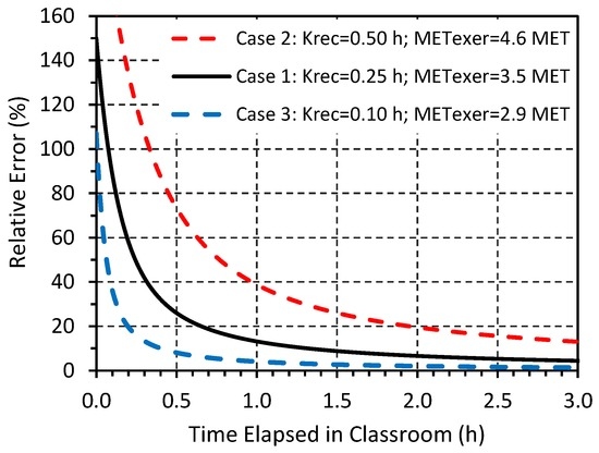
Figure 2.
Effect of post-exercise recovery on CO2 generation and metabolic activity rates, expressed as relative bias for periods of 0 to 3 h, compared to classroom activity of 1.4 MET. Assumes children undergoing light to moderate exercise (2.9 to 4.6 MET) prior to entering the classroom. Three cases shown: Case 1 uses nominal parameters; Case 2 uses “maximal effect” parameters; Case 3 uses “minimal effect” parameters.
While the analysis is approximate and uncertain given the data gaps (particularly those for children) and the simplified assumptions, results suggest that estimates of physical activity and thus GP applying to a student entering in a classroom will be underestimated if the preceding exercise is of high intensity (>4 METS) and the measurement time window is short (<1 or 2 h) and immediately follows the students’ entry into the classroom. To significantly affect the total CO2 generation rate, this must apply to most students entering the classroom. In such cases, the recovery effect will be significant and GP will be significantly underestimated, leading to an overestimate of the VR. The build-up method may be especially prone to the post-exercise recovery effect since it emphasizes the early portion of the CO2 trend; results for the transient mass balance and steady-state methods may also be affected, although smaller effects are expected since these methods tend to emphasize the higher CO2 concentrations that occur several hours after students enter the classroom. Figure 2 also suggests that the time window selected for analysis, if possible, should exclude the first hour after students enter the space. In many situations, however, the bias may be modest (<10%) even with considerable traffic into a classroom, a result of children’s quick recovery time (possibly underestimated since the analysis used the adult values), and since VR determinations typically use multihour-long time windows.
Examination of CO2 trends in the sample classrooms did not show evidence of post-exercise recovery effect, although effects could be obscured by other factors. In particular, physical activity levels might not be elevated prior to school since few children are walking or cycling to school. However, for students entering a classroom immediately following moderate to high level of physical activity from sports or other vigorous activity, METEXER may be particularly elevated, and thus the post-exercise recovery period should be excluded from the time window used to determine the VR.
3.3. Evaluation of the Methods
The sample of four classrooms in four schools was selected to demonstrate CO2-based methods, and results are not necessarily “representative” of elementary school classrooms. Still, results reflect a range of conditions, none of which appear to be exceptional, and they highlight several common issues in using CO2-based methods for determining VRs, based on the larger study [36]. First, occupancy levels vary considerably throughout the school day, and “clean” (and ideally prolonged) step-wise increases in occupancy were not seen in any of the classrooms. Instead, teachers arrived before students, students and teachers left for lunch, the number of students varied between morning and afternoon, and students generally entered and left in phases for classes and breaks. Second, VRs in the tested classrooms, all in modern mechanically-ventilated U.S. schools, are below recommended levels of 6.7 L·s−1·person−1 (assuming default occupancy and children ages 9 and up) [12]. This has been shown in other U.S. schools, e.g., V0 averaged 3.6 L·s−1·person−1 in elementary schools in the southwest U.S. (determined using CO2 and the steady-state method [8], and similar results have been reported in other countries [10,41]. Third, VRs were low (around 0.1 h−1) in the early morning (and generally the evening) when the building was not occupied, reflecting the shutdown of the ventilation system, and possibly a “tight” building envelope (Tightness was not measured in this study). Such energy and cost-savings measures, taken in the design and operation of many modern buildings, were anticipated for the EnergyStar buildings (Figure 1C,D), but also were apparent for the two conventional buildings tested (not designed to meet EnergyStar or other energy-certification system; Figure 1A,B). As discussed below, these issues have important consequences for VR estimates, which are below by method.
Often, the steady-state CO2 concentration CS in classrooms may not be reached, and CS can change over time, a result of low VRs and dynamic occupancy patterns. This was demonstrated in two of the classrooms (Figure 1A,D) that had ‘pointed’ peaks at the maximum CO2 concentration. In the two others (Figure 1B,C), CO2 trends began to plateau, an indication of the approach of steady-state conditions, but trends never became horizontal. The potential to overestimate VRs when the steady-state concentration is not attained has been recognized for many years, though this method continues to be widely used [26]. For CO2 measurements, we do not recommend averaging periods shorter than 5 to 10 min (or the use of instantaneous measurements) for CS, especially in schools and where instrumentation is unattended, given instrument noise and the possibility of unrepresentative spikes (e.g., children breathing on sensors). This also applies to CO2 measurements used in the build-up and other methods.
For classrooms that have just been vacated, CO2 levels tend to decline smoothly and exponentially, and decay and transient mass balance methods give comparable results. For the 2-point decay method (Equation (5)), selecting C0 and C1 as the maximum and minimum concentrations, respectively, within ±1 h of the nominal times for a 6 h time window, also gave similar estimates of AD as the nominal times. The decay method provided consistent results for evening and early morning time windows using 15-min average CO2 measurements and time windows as short as 2 h. However, VRs determined for the unoccupied period did not reflect conditions during the occupied period (see Section 2.2). Thus, decay-rate VRs may be less relevant to health and comfort investigations, although VRs estimated for the unoccupied period may relate to the build-up of emissions associated with building materials and furnishings (e.g., formaldehyde) and they may have energy-related and other implications.
The build-up method does not require steady-state conditions and can provide consistent results given a step-wise increase in CO2 generation rates. The method requires the identification of an appropriate time window, which must exclude changes in occupancy, and specifically the lunch period when students typically leave the classroom. Given patterns observed in the elementary schools, we recommend a nominal time window from 08:00 to 12:00 with flexible start and end times (±1 h) so as to minimize C0 and maximize C1. The classroom must be continuously occupied during the selected period. This protocol excludes the lunch hour and improves reliability. A 2 h time window was usually sufficient, which may allow analysis of both morning and afternoon build-up periods (again excluding the lunch period). Still, results can remain sensitive to the time window selected. This applied particularly to the ASTM and 3-point methods, which did not obtain consistent results, an unsurprising result given the irregularity of the observed build-up curves. In addition, the 3-point method failed when Equation (9) yielded a negative value of CS (as discussed in Section 2.3). Of the build-up methods, the implicit solution approach (Equations (10)–(12)) is recommended. This approach requires only two CO2 measurements, converged rapidly in each classroom tested using the modified Newton-Raphson method and the suggested starting solution, provided good stability, and obtained VR estimates that were more consistent with those of the transient mass balance method. However, this approach requires an estimate of occupancy over the sampling period. Only the morning period was used with the build-up method; longer periods gave poor outcomes due to occupancy changes. Even with the flexible start and stop times suggested, build-up air change rates provided by the implicit method were typically smaller (by 20% to 35%) than those calculated using the transient mass balance method, again, likely due to the irregular occupancy patterns. For each of the build-up methods, a CO2 concentration trend that follows the expected build-up curve is a necessary but not sufficient condition of a step-wise increase in occupancy and constant CO2 generation rate, assumptions of this method. To confirm results of the build-up method, the CO2 trend must follow the expected pattern, occupancy records must show a stepwise increase, and the physical activity level of students in the classroom must be constant. To minimize possible effects of the post-exercise recovery period, the selected time window might be lagged by at least one hour following periods when students undertake moderate to high intensity exercise, e.g., gym class.
The transient mass balance method, which uses a simple fully-mixed model and a straightforward optimization, yielded results that closely fitted observed CO2 levels in most cases. When occupancy patterns are irregular and steady-state levels are not achieved, the transient method generally provided larger and more potentially more accurate VRs than those from the steady-state and build-up methods. Because steady-state conditions or knowledge of CS are not required, and because all CO2 data are used (not just the measurements that border the analysis time window), the transient mass balance method may provide the most accurate and robust results among CO2-based methods for periods when classrooms are occupied. However, discrepancies can result from errors in reported occupancy and unknown activity levels of the children. Still, the overall agreement observed is excellent, demonstrating the feasibility and performance possible when using teacher−reported occupancy and 15-min block data. In most cases, results were not sensitive to the period selected, e.g., VRs for the 08:00 to 14:30 period were generally within 5% of those for the 08:00 to 16:00 period. Greater sensitivity can result if simulated and observed concentrations diverge (e.g., in the afternoon in Figure 1D), but this was the exception. As with the other methods, the time window should not bridge periods in which HVAC operation is changed.
3.4. Limitations
Several limitations apply to the methods and results. First, each room is assumed to be a single well-mixed zone that could be characterized by measurements at a central, but single location. Guidance for VR measurements using CO2 specifies that CO2 concentrations at representative locations should differ by less than 10% [24]. In the test classrooms, measurements that could evaluate this assumption were not obtained, but our experience in schools and other mechanically-ventilated spaces suggests that a central monitoring site is likely to provide measurements representative of the space. This is less likely when the HVAC system is turned off and mixing is reduced; however, the well-behaved decay curves as well as similar VRs determined for other classrooms in the same building at the same time [36] suggest that the CO2 measurements remained representative. The single zone model applied to classrooms has other limitations, e.g., classrooms can be connected together and HVAC zones can include hallways and other spaces in the building. In these cases, multizone models and additional parameters, e.g., multiple tracer gases and/or air flow measurements, may be needed to evaluate air change rates between building spaces as well as outdoors.
Second, measurements also need to be accurate, and errors will increase as CO2 levels decrease and approach outdoor levels. We did not evaluate the validity of the single zone assumption, i.e., interzone air and CO2 transport were neglected. Third, the steady-state and decay methods assumed that CO2 levels in replacement air CR are constant and known (or estimated), and the former method also requires attainment (or near-attainment) of steady-state CO2 levels. CO2 levels in replacement air should be based on contemporaneous outdoor measurements near the air intake of the space, thus accounting for possible differences in outdoor levels due to CO2 emissions from vehicle exhaust and other sources. Fourth, the decay, build-up and transient mass balance methods require measurements taken over a long enough period to observe a meaningful CO2 concentration change. This is rarely an issue in classrooms. Fifth, CO2 generation rates depend on the physical activity level of children in the classroom as well as the activity just prior to entering the classroom. The true activity level is unknown, may considerably exceed the default value assumed or the range considered, and may vary over time. This can affect VR estimates determined using the simulation, build-up and steady-state methods. Sixth, our analysis of the post-exercise recovery period was modeled, and supporting observations for children are not available. Further analysis of this issue is suggested. Seventh, each of the methods discussed require that the true VR does not change during the time window considered. As mentioned, VRs can vary for many reasons, especially in buildings that are naturally ventilated, that use variable air volume systems, that turn on or off HVAC systems during the time window, or if the infiltration rate varies during the time window (e.g., due to changes in outdoor temperatures and winds).
Examples were provided for a small set of classrooms with the intention of demonstrating the variability of CO2 patterns in schools. The sample is not necessarily representative. All studied classrooms were mechanically-ventilated and in relatively new buildings. We did not address day-to-day variability in the studied classrooms and among classrooms in the school, or quantify the uncertainty of results. However, we discussed uncertainties resulting from variations in occupant heights, weights and activity levels, occupancy data, method variation and the applicability of its assumptions, CO2 measurement errors, and the adequacy of mixing, among other factors.
Finally, it can be difficult to evaluate the performance of CO2-based and other methods to determine VRs. An independent and “reference” method, e.g., using a different and unique tracer gases or air flow measurements, was not utilized to confirm the results. Even these methods involve many assumptions and few if any intercomparisons of different methods have been conducted in parallel measurements under real-life conditions [15]. While VRs were estimated using information obtained from HVAC drawings, schedules and manufacturer’s material, this information was incomplete and does not necessarily reflect actual performance. In all cases, even the minimum VRs estimated using this information consistently exceeded the in-use VRs determined using the CO2-based methods.
4. Conclusions
Ventilation rates are critical parameters that relate to building energy performance and the health and comfort of occupants. Ventilation rates determined using CO2-based methods, which are commonly applied, were reviewed and critiqued, with special attention to classroom applications. The methods were demonstrated in primary school classrooms in modern and mechanically-ventilated buildings. As shown in the literature, ventilation rates in the tested classrooms during the school day fell below minimum recommendations. Air change rates during evening and early morning, when the ventilation system was shut down, were far lower (around 0.1 h−1).
VRs determined using transient mass balance methods are flexible, robust and advantageous given the low VRs and dynamic occupancy patterns often found in classrooms. These methods require information pertaining to changes in occupancy, some basic building and occupancy parameters, and numerical methods to estimate air change rates. Several updates to the build-up method were presented, namely, an implicit method to find AB and CS simultaneously using occupancy information, and an adaptive approach to selecting the analysis time window. The utility of the steady-state and build-up methods may be limited in classrooms for several reasons: the steady-state CO2 concentration may not be reached, measured or estimated accurately; a step-wise increase in occupancy may not be observed or confirmed; and post-exercise recovery can alter the CO2 generation rate, particularly with vigorous physical activity immediately prior to entering a classroom. During unoccupied periods, the decay and transient mass balance methods can provide equivalent results, however, VRs determined for such periods will not be representative of the occupied portion of the school day if the HVAC system is shut-down or a VAV system is utilized and the heating or cooling load changes significantly when occupants leave. In the schools examined, most HVAC systems were shut down immediately after students left. Thus, VRs determined at the end of the school day will likely be of less interest for many types of building investigations.
If occupancy measurements can be obtained, then VRs determined using transient mass balance methods will provide the most accurate and robust results. Without occupancy measurements, CO2 concentration trends must be carefully examined to determine whether the steady-state or build-up method can be used, and to determine an appropriate time window for analysis. Still, sufficient occupancy data should be collected to confirm that the method’s assumptions and results are correct. Better VR measurements would improve a number of applications, including research aimed at understanding the linkage between ventilation and health.
Supplementary Materials
The following are available online at www.mdpi.com/1660-4601/14/2/145/s1, Figure S1: Trends of a child’s activity level and the relative bias, showing the effect of the recovery period following exercise. The instantaneous MET trend is predicted using Equation (19). The average MET trend averages the instantaneous MET levels back to time t = 0. The relative error represents the difference between the average MET level (accounting for the recovery period) and the sedentary MET level (1.4 MET). Three cases are shown. Case 1 uses nominal values of recovery time and exercise activity. Case 2 uses parameters selected to have a “maximal effect” on MET predictions. Case 3 uses parameters selected to have a “minimal effect” on MET predictions. The Supplementary Materials also presents the full solution for the implicit build-up method. The author will gladly share an Excel workbook that clearly demonstrates each of the methods discussed, and a second macro-enabled Excel workbook that demonstrates the calculations and produces the graphics in this paper. Please contact the author.
Acknowledgments
We appreciate the participation and assistance of the teachers and staff at each school. We thank our research staff, including Andrew Wald, Christopher Godwin, Floyd Watkins, Geoffrey Thun, Lexuan Zhong, Feng-Chiao Su, Nicole Mitchell, Julien Heidt and An Nguyen for their assistance. The reviewers provided helpful comments. This publication was developed under Assistance Agreement No. is 83563701−0 awarded by the U.S. Environmental Protection Agency to the University of Michigan. It has not been formally reviewed by EPA. EPA does not endorse any products or commercial services mentioned in this publication. Additional support for this research was provided by grant P30ES017885 from the National Institute of Environmental Health Sciences, National Institutes of Health. The content is solely the responsibility of the authors and does not necessarily represent the official views of the EPA or the National Institutes of Health.
Conflicts of Interest
The author declares no conflict of interest.
References
- Haverinen-Shaughnessy, U.; Moschandreas, D.J.; Shaughnessy, R.J. Association between substandard classroom ventilation rates and students’ academic achievement. Indoor Air 2011, 21, 121–131. [Google Scholar] [CrossRef] [PubMed]
- Shendell, D.G.; Prill, R.; Fisk, W.J.; Apte, M.G.; Blake, D.; Faulkner, D. Associations between classroom CO2 concentrations and student attendance in Washington and Idaho. Indoor Air 2004, 14, 333–341. [Google Scholar] [CrossRef] [PubMed]
- Wargocki, P.; Wyon, D.P. The effects of outdoor air supply rate and supply air filter condition in classrooms on the performance of schoolwork by children (rp-1257). HVAC&R Res. 2007, 13, 165–191. [Google Scholar]
- Sundell, J.; Bronswijk, V.J.; Dijken, V.F. Indoor environment and pupils’ health in primary schools. Build. Res. Inform. 2006, 34, 437–446. [Google Scholar]
- Sundell, J.; Levin, H.; Nazaroff, W.W.; Cain, W.S.; Fisk, W.J.; Grimsrud, D.T.; Gyntelberg, F.; Li, Y.; Persily, A.K.; Pickering, A.C.; et al. Ventilation rates and health: Multidisciplinary review of the scientific literature. Indoor Air 2011, 21, 191–204. [Google Scholar] [CrossRef] [PubMed]
- Mendell, M.J.; Eliseeva, E.A.; Davies, M.M.; Spears, M.; Lobscheid, A.; Fisk, W.J.; Apte, M.G. Association of classroom ventilation with reduced illness absence: A prospective study in California elementary schools. Indoor Air 2013, 23, 515–528. [Google Scholar] [CrossRef] [PubMed]
- Rosbach, J.T.M.; Vonk, M.; Duijm, F.; van Ginkel, J.T.; Gehring, U.; Brunekreef, B. A ventilation intervention study in classrooms to improve indoor air quality: The FRESH study. Environ. Health 2013, 12, 110. [Google Scholar] [CrossRef] [PubMed]
- Haverinen-Shaughnessy, U.; Shaughnessy, R.J. Effects of classroom ventilation rate and temperature on students’ test scores. PLoS ONE 2015, 10, e0136165. [Google Scholar] [CrossRef] [PubMed]
- Gaihre, S.; Semple, S.; Miller, J.; Fielding, S.; Turner, S. Classroom carbon dioxide concentration, school attendance, and educational attainment. J. Sch. Health 2014, 84, 569–574. [Google Scholar] [CrossRef] [PubMed]
- Chatzidiakou, L.; Mumovic, D.; Summerfield, A.J. What do we know about indoor air quality in school classrooms? A critical review of the literature. Intell. Build. Int. 2012, 4, 228. [Google Scholar] [CrossRef]
- Pérez-Lombard, L.; Ortiz, J.; Pout, C. A review on buildings energy consumption information. Energy Build. 2008, 40, 394–398. [Google Scholar] [CrossRef]
- ASHRAE. ANSI/ASHRAE Standard 62.1-2013, Ventilation for Acceptable Indoor Air Quality; American Society of Heating, Refrigerating and Air-Conditioning Engineers, Inc.: Atlanta, GA, USA, 2013. [Google Scholar]
- Persily, A.K. Field measurement of ventilation rates. Indoor Air 2016, 26, 97–111. [Google Scholar] [CrossRef] [PubMed]
- Persily, A.K.; Gorfain, J.; Brunner, G. Survey of ventilation rates in office buildings. Build. Res. Inform. 2006, 34, 459–466. [Google Scholar] [CrossRef]
- Sherman, M.H. Tracer-gas techniques for measuring ventilation in a single zone. Build. Environ. 1990, 25, 365–374. [Google Scholar] [CrossRef]
- ASTM. Standard Test Method for Determining Air Change in a Single Zone by Means of a Tracer Gas Dilution; ASTM International: West Conshohocken, PA, USA, 2011. [Google Scholar]
- ISO. ISO 12569:2012: Thermal Performance of Buildings and Materials—Determination of Specific Airflow Rate in Buildings—Tracer Gas Dilution Method; International Organization for Standardization: Geneva, Switzerland, 2012; p. 54. [Google Scholar]
- Etheridge, D. Natural Ventilation of Buildings: Theory, Measurement and Design; John Wiley & Sons Inc./Wiley Wiley-Blackwell: West Sussex, UK, 2012. [Google Scholar]
- Bekö, G.; Gustavsen, S.; Frederiksen, M.; Bergsøe, N.C.; Kolarik, B.; Gunnarsen, L.; Toftum, J.; Clausen, G. Diurnal and seasonal variation in air exchange rates and interzonal airflows measured by active and passive tracer gas in homes. Build. Environ. 2016, 104, 178–187. [Google Scholar] [CrossRef]
- Chatzidiakou, E. Is CO2 A Good Proxy for Indoor Air Quality in School Classrooms? ProQuest Dissertations Publishing: London, UK, 2014. [Google Scholar]
- Hänninen, O.; Shaughnessy, R.; Turk, B.; Egorov, A. Evaluation of Ventilation Rates in European Schools Using CO2 Measurements as Part of a Proposed WHO School Survey; Healthy Buildings: Brisbane, Australia, 2012. [Google Scholar]
- Scheff, P.A.; Paulius, V.K.; Huang, S.W.; Conroy, L.M. Indoor air quality in a middle school, part I: Use of CO2 as a tracer for effective ventilation. Appl. Occup. Environ. Hyg. 2000, 15, 824–834. [Google Scholar] [CrossRef] [PubMed]
- Smith, P.N. Determination of ventilation rates in occupied buildings from metabolic CO2 concentrations and production rates. Build. Environ. 1988, 23, 95–102. [Google Scholar] [CrossRef]
- ASTM. Standard Guide for Using Indoor Carbon Dioxide Concentrations to Evaluate Indoor Air Quality and Ventilation; ASTM International: West Conshohocken, PA, USA, 2012. [Google Scholar]
- Hänninen, O. Novel second-degree solution to single zone mass-balance equation improves the use of build-up data in estimating ventilation rates in classrooms. J. Chem. Health Saf. 2013, 20, 14–19. [Google Scholar] [CrossRef]
- Mudarri, D.H. Potential correction factors for interpreting CO2 measurements in buildings. ASHRAE Trans. 1997, 103, 244–254. [Google Scholar]
- Carrilho, J.D.; Mateus, M.; Batterman, S.; da Silva, M.G. Air exchange rates from atmospheric CO2 daily cycle. Energy Build. 2015, 92, 188–194. [Google Scholar] [CrossRef] [PubMed]
- Hänninen, O.O.; Lebret, E.; Ilacqua, V.; Katsouyanni, K.; Künzli, N.; Srám, R.J.; Jantunen, M. Infiltration of ambient PM2.5 and levels of indoor generated non-ETS PM2.5 in residences of four European cities. Atmos. Environ. 2004, 38, 6411–6423. [Google Scholar]
- ASTM. E779-10 Standard Test. Method for Determining Air Leakage Rate by Fan Pressurization; American Society for Testing and Materials: West Conshohocken, PA, USA, 2010. [Google Scholar]
- Du, L.; Batterman, S.; Godwin, C.; Chin, J.-Y.; Parker, E.; Breen, M.; Brakefield, W.; Robins, T.; Lewis, T. Air change rates and interzonal flows in residences, and the need for multi-zone models for exposure and health analyses. Int. J. Environ. Res. Public Health 2012, 9, 4639–4662. [Google Scholar] [CrossRef] [PubMed]
- Carrer, P.; Wargocki, P.; Fanetti, A.; Bischof, W.; De Oliveira Fernandes, E.; Hartmann, T.; Kephalopoulos, S.; Palkonen, S.; Seppänen, O. What does the scientific literature tell us about the ventilation-health relationship in public and residential buildings? Build. Environ. 2015, 94, 273–286. [Google Scholar] [CrossRef]
- Hänninen, O. Combining CO2 Data from Ventilation Phases Improves Estimation of Air Exchange Rates; Healthy Buildings: Brisbane, Australia, 2012. [Google Scholar]
- WHO. Methods for Monitoring Indoor Air Quality in Schools: Report from the Meeting 4–5 April 2011 Bonn, Germany; World Health Organization: Copenhagen, Denmark, 2011; p. 32. [Google Scholar]
- George, K.; Ziska, L.H.; Bunce, J.A.; Quebedeaux, B. Elevated atmospheric CO2 concentration and temperature across an urban-rural transect. Atmos. Environ. 2007, 41, 7654–7665. [Google Scholar] [CrossRef]
- Yasuda, T.; Yonemura, S.; Tani, A. Comparison of the characteristics of small commercial NDIR CO2 sensor models and development of a portable CO2 measurement device. Sensors 2012, 12, 3641–3655. [Google Scholar] [CrossRef] [PubMed]
- Batterman, S.; Su, F.-C.; Wald, A.; Watkins, F.; Godwin, C.; Thun, T. Ventilation rates in recently constructed U.S. elementary school classrooms. Indoor Air 2017. under review. [Google Scholar]
- Breen, M.S.; Schultz, B.D.; Sohn, M.D.; Long, T.; Langstaff, J.; Williams, R.; Isaacs, K.; Meng, Q.Y.; Stallings, C.; Smith, L. A review of air exchange rate models for air pollution exposure assessments. J. Expo. Sci. Environ. Epidemiol. 2014, 24, 555–563. [Google Scholar] [CrossRef] [PubMed]
- Lawrence, T.M. Selecting CO2 criteria for outdoor air monitoring. ASHRAE J. 2008, 50, 18. [Google Scholar]
- Morse, R.G.; Haas, P.; Lattanzio, S.M.; Zehnter, D.; Divine, M. A cross-sectional study of schools for compliance to ventilation rate requirements. J. Chem. Health Saf. 2009, 16, 4–10. [Google Scholar] [CrossRef]
- You, Y.; Niu, C.; Zhou, J.; Liu, Y.; Bai, Z.; Zhang, J.; He, F.; Zhang, N. Measurement of air exchange rates in different indoor environments using continuous CO2 sensors. J. Environ. Sci. 2012, 24, 657–664. [Google Scholar] [CrossRef]
- Turanjanin, V.; Vutiaevic, B.; Jovanovic, M.; La Mirkov, N.; Lazovic, I. Indoor CO2 measurements in Serbian schools and ventilation rate calculation. Energy 2014, 77, 290–296. [Google Scholar] [CrossRef]
- Mundt, E.; Mathisen, H.M.; Nielsen, P.V.; Moser, A. Ventilation Effectiveness; REHVA Federation of European Heating Ventilation and Air Conditioning Associations: Brussels, Belgium, 2004. [Google Scholar]
- Canha, N.; Mandin, C.; Ramalho, O.; Wyart, G.; Ribéron, J.; Dassonville, C.; Hänninen, O.; Almeida, S.M.; Derbez, M. Assessment of ventilation and indoor air pollutants in nursery and elementary schools in France. Indoor Air 2016, 26, 350–365. [Google Scholar] [CrossRef] [PubMed]
- Hänninen, O.; Canha, N.; Dume, I.; Deliu, A.; Mata, E.; Egorov, A. P-217. Epidemiology 2012, 23, 1. [Google Scholar] [CrossRef]
- Penman, J.M. An experimental determination of ventilation rate in occupied rooms using atmospheric carbon dioxide concentration. Build. Environ. 1980, 15, 45–47. [Google Scholar] [CrossRef]
- Mumovic, D.; Palmer, J.; Davies, M.; Orme, M.; Ridley, I.; Oreszczyn, T.; Judd, C.; Critchlow, R.; Medina, H.A.; Pilmoor, G.; et al. Winter indoor air quality, thermal comfort and acoustic performance of newly built secondary schools in England. Build. Environ. 2009, 44, 1466–1477. [Google Scholar] [CrossRef]
- Santamouris, M.; Synnefa, A.; Asssimakopoulos, M.; Livada, I.; Pavlou, K.; Papaglastra, M.; Gaitani, N.; Kolokotsa, D.; Assimakopoulos, V. Experimental investigation of the air flow and indoor carbon dioxide concentration in classrooms with intermittent natural ventilation. Energy Build. 2008, 40, 1833–1843. [Google Scholar] [CrossRef]
- National Center for Health Statistics. Percentile Data Files with LMS Values, CDC Growth Charts. Available online: http://www.cdc.gov/growthcharts/percentile_data_files.htm (accessed on 1 October 2016).
- U.S. Environmental Protection Agency. Exposure Factors Handbook: 2011 Edition; U.S. Environmental Protection Agency: Washington, DC, USA, 2011.
- Saint-Maurice, P.F.; Kim, Y.; Welk, G.J.; Gaesser, G.A. Kids are not little adults: What MET threshold captures sedentary behavior in children? Eur. J. Appl. Physiol. Occup. Phys. 2016, 116, 29–38. [Google Scholar] [CrossRef] [PubMed]
- Ridley, K.; Ainsworth, B.E.; Olds, T.S. Development of a compendium of energy expenditures for youth. Int. J. Behav. Nutr. Phys. Act. 2008, 5, 45. [Google Scholar] [CrossRef] [PubMed]
- Ainsworth, B.E.; Haskell, W.L.; Herrmann, S.D.; Meckes, N.; Bassett, D.R., Jr.; Tudor-Locke, C.; Greer, J.L.; Vezina, J.; Whitt-Glover, M.C.; Leon, A.S. 2011 compendium of physical activities: A second update of codes and MET values. Med. Sci. Sports Exerc. 2011, 43, 1575–1581. [Google Scholar] [CrossRef] [PubMed]
- Buchheit, M.; Laursen, P.B.; Ratel, S.; Duché, P. Postexercise heart rate recovery in children: Relationship with power output, blood pH, and lactate. Appl. Physiol. Nutr. Metab. 2010, 35, 142–150. [Google Scholar] [CrossRef] [PubMed]
- Compher, C.; Frankenfield, D.; Keim, N.; Roth-Yousey, L. Best practice methods to apply to measurement of resting metabolic rate in adults: A systematic review. J. Am. Diet. Assoc. 2006, 106, 881–903. [Google Scholar] [CrossRef] [PubMed]
- Laforgia, J.; Withers, R.T.; Gore, C.J. Effects of exercise intensity and duration on the excess post-exercise oxygen consumption. J. Sports Sci. 2006, 24, 1247–1264. [Google Scholar] [CrossRef] [PubMed]
© 2017 by the author. Licensee MDPI, Basel, Switzerland. This article is an open access article distributed under the terms and conditions of the Creative Commons Attribution (CC BY) license ( http://creativecommons.org/licenses/by/4.0/).