Article

Mobile Measurements of Particulate Matter in a Car Cabin: Local Variations, Contrasting Data from Mobile versus Stationary Measurements and the Effect of an Opened versus a Closed Window

1
Institute of Occupational, Social, and Environmental Medicine, Goethe University Frankfurt, Theodor-Stern-Kai 7, 60590 Frankfurt am Main, Germany
2
Institute of Occupational Medicine, Charité–School of Medicine, Humboldt-University & Free University, Augustenburger Platz 1, 13353 Berlin, Germany
*
Author to whom correspondence should be addressed.
Int. J. Environ. Res. Public Health 2018, 15(12), 2642; https://doi.org/10.3390/ijerph15122642
Submission received: 24 October 2018 / Revised: 20 November 2018 / Accepted: 21 November 2018 / Published: 26 November 2018
(This article belongs to the Special Issue Transportation-Related Air Pollution and Human Health)

Abstract

:
Air pollution of particulate matter (PM) from traffic emissions has a significant impact on human health. Risk assessments for different traffic participants are often performed on the basis of data from local air quality monitoring stations. Numerous studies demonstrated the limitation of this approach. To assess the risk of PM exposure to a car driver more realistically, we measure the exposure to PM in a car cabin with a mobile aerosol spectrometer in Frankfurt am Main under different settings (local variations, opened versus a closed window) and compare it with data from stationary measurement. A video camera monitored the surroundings for potential PM source detection. In-cabin concentrations peaked at 508 µg m−3 for PM10, 133.9 µg m−3 for PM2.5, and 401.3 µg m−3 for coarse particles, and strongly depended on PM size and PM concentration in ambient air. The concentration of smaller particles showed low fluctuations, but the concentration of coarse particles showed high fluctuations with maximum values on busy roads. Several of these concentration peaks were assigned to the corresponding sources with characteristic particle size distribution profiles. The closure of the car window reduced the exposure to PM, and in particular to coarse particles. The mobile measured PM values differed significantly from stationary PM measures, although good correlations were computed for finer particles. Mobile rather than stationary measurements are essential to assess the risk of PM exposure for car passengers.

1. Introduction

Urban agglomeration areas are usually characterized by a high rate of air pollution caused by particulate matter (PM). In urban areas, PM is mainly emitted by cars burning fossil fuel or during abrasion processes of vehicle tires and brakes, respectively, from raised dust. Further sources are power plants and chemical or metallurgical factories [1,2]. Very high concentrations can especially be reached nearby roads [3]. PM can contain particles with a lot of different sizes [4]. For monitoring air quality, usually the particle fractions PM10 (particulate matter with an aerodynamic diameter less than 10 µm), PM2.5 (particulate matter with an aerodynamic diameter less than 2.5 µm), and PM1 (particulate matter with an aerodynamic diameter less than 1 µm) are used. Particles with an aerodynamic diameter between 2.5 and 10 µm belong to coarse fraction (PMcoarse) [5]. High exposures of PM have negative consequences for human health and are therefore a key issue in current research [6]. Already, very low concentrations of PM can increase the blood pressure or raise the risk of cardiovascular diseases [7]. Recent research showed that even short-term exposures with very high PM concentrations, which are typical for traffic participants, can be harmful to health [8,9,10]. Under long-term exposure, the consequences can be even worse. The probability for the formation of lung carcinomas increases [11]. A long-term exposure can also negatively affect fetal growth or changes heart rate variability [12,13,14,15,16]. Due to increased health risks, especially in urban areas, where anthropogenic emissions of PM are the highest, further research is obligatory. Many cities have a system of air quality monitoring stations (AQMS) for getting an overview of the local PM pollution [17]. The AQMS data is often used to estimate the PM exposure for society. Based on this knowledge, guidelines are created and political decisions are made [18]. Because AQMS measurements are only for outside air and the PM concentration with its respective sources is generally distributed very heterogeneously within a certain area, it is questionable whether these static measurements are generally suitable for estimating the actual exposure to traffic participants, especially to passengers inside a car [19,20,21,22]. In Germany, for example, people spend, on average, 1 h and 28 min a day travelling, depending on their occupation and residence, mainly in cars [23]. Some occupation groups, such as taxi or courier drivers, spend even more time in their cars. During that driving time, most of the daily PM uptake is made [24,25,26]. Because of such a high medical relevance, monitoring PM concentrations in the driver cabin is an essential research field. Frankfurt am Main, the study site in the presented study, is predestinated for a mobile air quality study because of its extremely high commuter traffic and a population density of almost 3000 people/km². This value is one of the highest in Germany [27]. In the course of this study, local and temporal variations of PM concentrations and particle sizes in the cabin of a car were characterized while driving on an urban circular drive in Frankfurt am Main. Furthermore, the PM concentration and the particle size distribution from rides with an opened window (OW) and closed window (CW) have been compared with each other. By comparing the measured data in a car cabin with AQMS data, the suitability of the AQMS data for estimating the actual PM exposure for a driver was tested to assess his potential health risk from exposure to traffic-related PM.

2. Materials and Methods

2.1. Measurement of Particulate Matter

Car rides for the mobile air quality study were made with an electric vehicle of the BMW i3 model with the intention to avoid an exhaust related increase of in-cabin PM concentration by the car itself. The PM in-cabin concentration was measured by an aerosol spectrometer, type GRIMM 11-R. It was used according to the quality guidelines of the supplier and calibrated before the measurement. The suction of the instrument was placed at the co-driver’s seat at head height to get a realistic image of the actual PM exposure to the driver in the cabin. The spectrometer was connected to a laptop (Fujitsu Lifebook) and a GPS (Global Positioning System) mouse. Every six seconds, a value was generated for the fractions, PM10, PM2.5, and PM1. The measured PM data was linked to the corresponding localization, velocity, and distance run. Data were visualized by converting them into a kml file (Keyhole Markup Language) and by the use of Google Earth (Figure 1).
In addition to the PM measurement, a camera was recording the surroundings of the car for further identifications of potential PM sources at concentration peaks of PM.

2.2. Driving Routes

In our experimental set up, two different types of routes were driven. Each of them was focusing on certain problems. Local differences in PM concentration and particle size distribution in the driver’s cabin were analyzed on a 15 km circular drive through Frankfurt am. PM concentration differences depending on the ventilation mode (opened window vs. closed window) were quantified on a circular drive in a residential area.

2.2.1. In-Cabin PM Concentration (Local Differences in Concentration and Particle Size Distribution)

Local differences in PM concentration and particle size distribution in the driver’s cabin were analyzed on a 15 km circular drive through Frankfurt am Main (Course 1; Figure 2).
To collect representative data of the commuter traffic, the route included minor roads, main roads, and a part of a high way. Furthermore, test rides were run on different days of the week before, during, and after rush hour. At peak times, there were numerous traffic jams within the city, especially at traffic lights. Thus, there is a maximum difference in the round time of 17 min (Table 1), with an average round time of 38 min. The test rides were run with different ventilation modes (opened window/closed window).
During the rides with opened window (OW), the window was halfway down and the air conditioning (AC) was switched off. During rides with closed window (CW), the ventilation of the AC was turned on at half of the power with a temperature of 20 °C. A ventilation break of 3 min was made after every ride with OW.
For comparison of the PM data from mobile measurement with AQMS data, the course was chosen to pass the AQMS “Friedberger Landstraße” located at a high-traffic point in Frankfurt am Main. Open-source PM data from the AQMS “Friedberger Landstraße” were downloaded from the homepage from Hessisches Landesamt für Naturschutz, Umwelt und Geologie (HLNUG).
Course 1 was run repeatedly on nine different days between May 2015 and January 2016. Driving dates, intervals, and the point of time while passing the AQMS are given for Course 1 in Table 1.

2.2.2. In-Cabin PM Concentration—Opened Window versus Closed Window

For better quantification of in-cabin PM concentration differences depending on the ventilation mode (OW vs. CW), a different test location was chosen (Course 2; Figure 3).
In this context, it must be ensured that external conditions, like weather or traffic volume, did not change significantly while concentrations from two following rides were compared with each other. For this purpose, a circular drive in a residential area was chosen. On this much shorter route, with a speed limit of 30 km/h, the traffic volume is very low. The route consisted mainly of one-way streets. Other driving vehicles were only rarely in direct proximity to our test vehicle. The driving time was mostly identical (Table 2). The influence of potential point sources, which lead to high short-term PM concentrations and falsifications in the analyses, were therefore minimized. Nevertheless, the location between two main roads represented the urban traffic influence. The interval between opened window and closed rides was consequently limited to 15 min, so it can be assumed that the background PM concentration did not vary significantly. For the comparison, an alternation between driving with OW and CW was made. During the rides with OW, the window was halfway down and the AC was switched off. During rides with CW, the ventilation of the AC was turned on at half of the power with a temperature of 20 °C. A ventilation break of 3 min was made after every ride with OW. This course was run eight times on each of the four dates. The date and time intervals for the rides in the residential area are listed in Table 2.

2.3. Statistics

The local PM concentration and particle size distribution measured inside the cabin were analyzed based on mobile measured PM values with a 6-s resolution.
To discriminate between the short-term concentration peaks of PM and the background concentration, both components must be separated from each other. Percentile-filters were applied on PM values because they eliminate strongly fluctuating short-term concentration peaks, but maintain the slowly changing background concentration. The use of 5%-percentiles (the average of the 5%-lowest values for a certain period) is widely accepted for mobile outdoor measurements [28]. Although the measurements in this study took place inside the cabin, the application of the 5%-percentile seemed to be an adequate method to gain a clear discrimination between both PM trends. For this specific experimental set-up, the velocity driven and the length of the circular drive with an interval of three minutes was used. The 3-min-5%-percentile was computed with R and the graphical presentation was made with Graphpad Prism. The coefficient of variation (CV) was calculated as a dimension for the general concentration inhomogeneity measured in the car while driving through the urban area.
For the comparison between the PM concentrations measured inside the car and the PM concentrations measured by the AQMS, two different approaches were applied.
For each test ride on the 15 km circular drive (Course 1), a mean value (PMmean) of the mobile measurement was calculated for PM10, PM2.5, and PMcoarse. Because the AQMS does not provide data for PM1, a comparison in this particle size category was not possible.
Furthermore, PM values of the period of time, when the car passes the AQMS (PMdirect), were computed for all particle fractions based on the GPS-data and kml files. PMdirect also is a PM average measured 30 s before and 30 s after the AQMS was passed. Both, PMmean and PMdirect, were compared to the chronological fitting PM data of the AQMS. A slight deviation could not be avoided because the highest resolution of the AQMS data is given for a 0.5 h mean value. Possible correlations between the PM values from the mobile measurement and the values of the AQMS were analyzed with the Spearman-test and p-values were calculated. Additionally, the quotients, PMmean/PMAQMS and PMdirect/PMAQMS, were calculated. These ratios reveal PM concentration differences and show whether the mobile measured values relate to the AQMS values. In combination with the corresponding coefficients of variation, the ratios show whether a statement about the driver’s PM exposure based on AQMS measurements can be made. For the analyses of single point sources, size particles were grouped in the categories of 2.5–10 µm, 1–2.5 µm, and <1 µm. For the calculation of the range of particles with diameters between 2.5 and 10 µm, the PM2.5 concentration was subtracted from the PM10 concentration. For the range of particles with a diameter between 1 and 2.5 µm, the PM1 concentration was subtracted from the PM2.5 concentration.
In order to compare in-cabin PM concentrations from OW rides with CW rides (Course 2; Figure 3), the median for each test ride was calculated. The medians of the test rides were compared with each other in a rank-based Mann-Whitney U-Test and p-values were calculated. In this case, the medians were used as robust values to minimize the influence of short-term concentration peaks, which are typical for single point sources. Particles have been grouped in the categories of 2.5–10 µm, 1–2.5 µm, and <1 µm. The medians of every consecutive opened window-closed window ride were analyzed and compared. The PM reduction achieved by closing the window was calculated separately for each fraction. Finally, the average PM reduction after closing the window was made for each of the four driving days.

3. Results

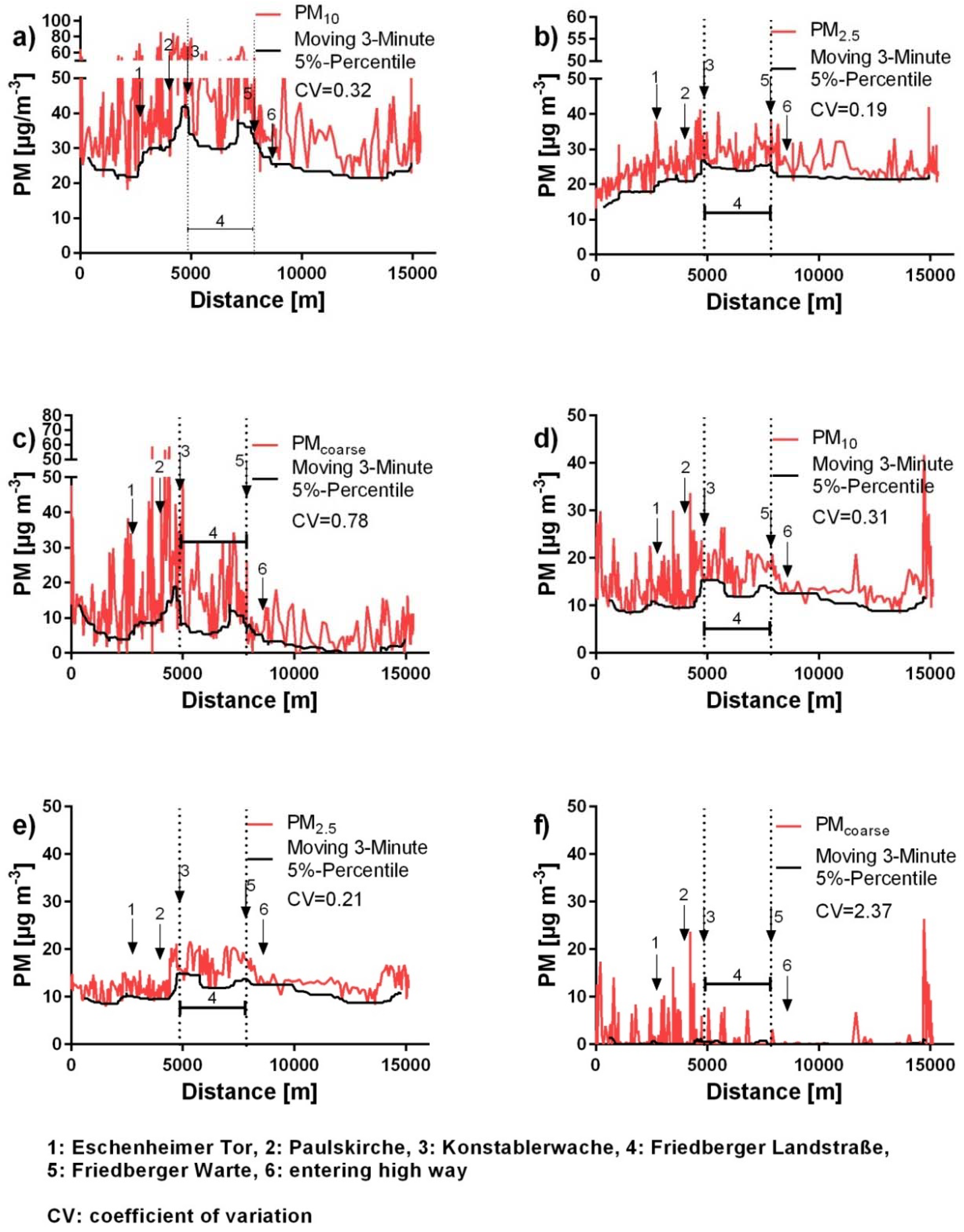
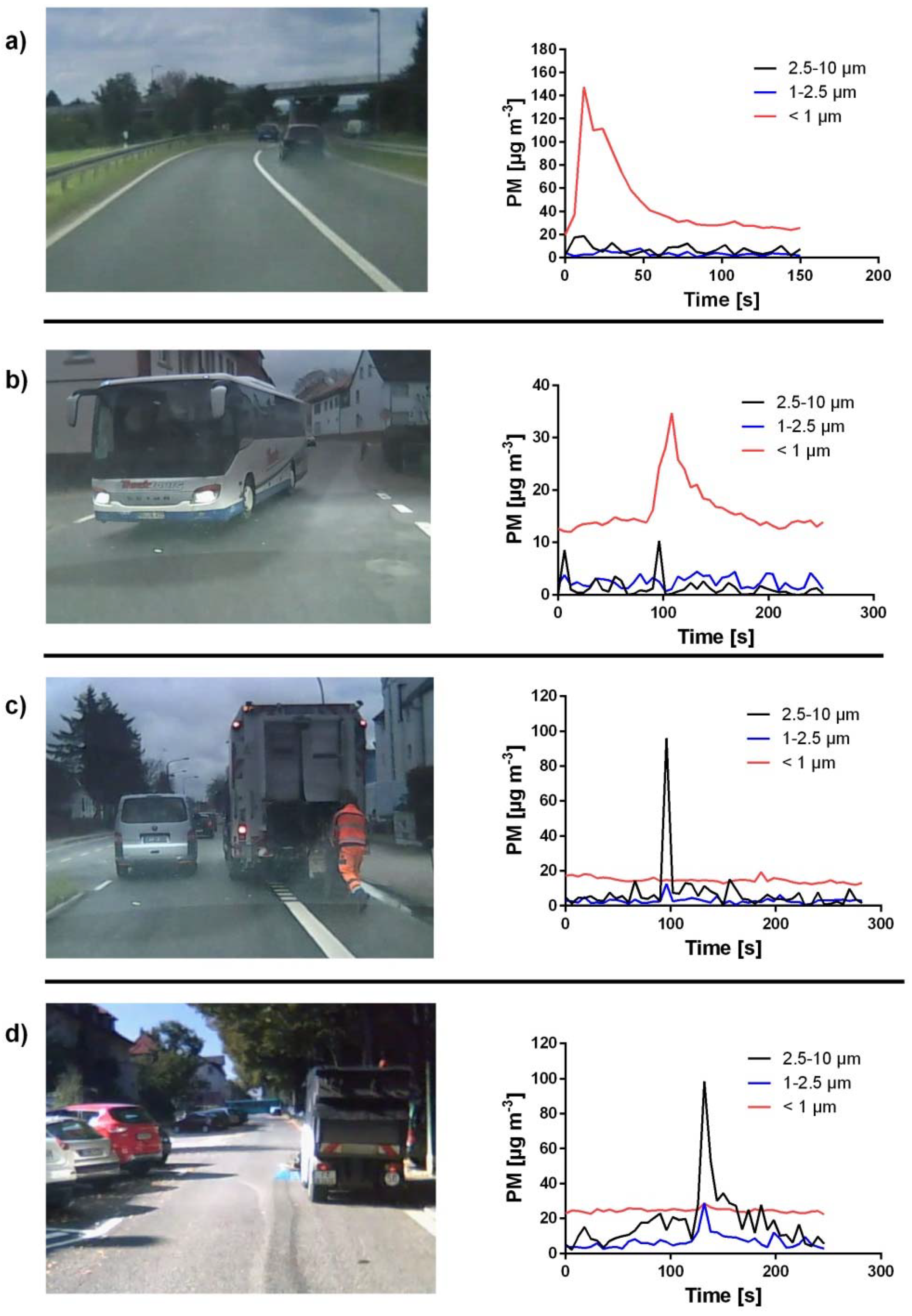
3.1. Local Variations of In-Cabin PM Concentrations and Particle Size Distribution

During the circular drive on Course 1 (Figure 2), maximum OW-concentrations of 508.9 µg m−3 for PM10 (Figure 4a), 401.3 µg m−3 for PMcoarse (Figure 4a), 133.9 µg m−3 for PM2.5 (Figure 4b), and 122.9 µg m−3 for PM1 (Figure 4b) were measured. Figure 4 shows examples for significantly high concentrations measured during the whole period of this study with a subdivision in different particle size fractions.
Those short-term concentration peaks generally lasted only seconds or a few minutes. The particle spectrums of these peaks show strong variations. While driving with CW, the concentration pattern was similar, but with lower values of 85.1 µg m−3 for PM10, 30.3 µg m−3 for PMcoarse, 85.0 µg m−3 for PM2.5, and 84.6 µg m−3 for PM1.
By visualizing the alternation of the local PM background concentrations measured in the car while driving within the city, characteristic trends were observed (Figure 5).
The PM10 background concentrations under OW conditions are slightly changing during the circular drive. The highest concentrations are mainly measured in the city center and the area of “Friedberger Landstraße”. The signal of the absolute PM10 concentration shows numerous short-term peaks.
The pattern of the background concentrations of PM2.5 and PM1 show an increase in the beginning and subsequently stay on approximately the same level. The absolute concentration levels reveal several short-term peaks, but less in frequency and magnitude, than in the PM10 signal.
The pattern of the background concentrations of PMcoarse vary strongly. The highest concentrations under opened window conditions are mainly measured in the city center and in the area of “Friedberger Landstraße”.
The median coefficient of variation of all rides with OW is 0.32 for PM10, 0.20 for PM2.5, 0.18 for PM1, and 1.04 for PMcoarse (n = 14).
While driving with a closed window, the pattern of the background concentrations of PM10, PM2.5, and PM1 show a similar trend. They stay approximately on the same level and reach their highest concentrations in the city center.
The CW profiles also show several short-term concentration peaks. The profiles of PMcoarse do not show any trends. Only isolated concentration peaks were monitored irregularly. A relation to specific locations in the city was not observed. The median coefficients of variation are 0.30 for PM10, 0.21 for PM2.5, 0.22 for PM1, and 3.07 for PMcoarse (n = 12).
The additional evaluation of the video material allowed the assignment of several short-term concentration peaks to the corresponding sources (Figure 6).
While driving behind a street sweeper or a garbage truck, particles with a diameter between 2.5 and 10 µm dominated. While driving behind a bus or a car with soot production, particles smaller than 1 µm were measured almost exclusively.
These observations were only made while driving with an opened window. In contrast, short-term concentration peaks could not distinctively be connected to any ambient sources while driving with a closed window.

3.2. PM In-Cabin versus PM AQMS

Table 3 summarizes the mobile measured in-cabin PM concentrations (PMmean, PMdirect) on the 15 km urban circular drive, Course 1 (Figure 2), with the chronological fitting PM data from the AQMS (PMAQMS) for the different particle size fractions and driving modes.
Correlations between PMmean and PMAQMS, respectively, between PMdirect and PMAQMS are given in Table 4. Rides with OW and rides with CW are analyzed separately.
In-cabin PMmean concentrations correlate significantly with the PM concentrations measured at stationary by the AQMS for the particle fractions, PM10 and PM2.5. The best correlation between PMmean and PMAQMS was observed for the fraction, PM2.5. There was no correlation between PMmean and PMAQMS for the fraction, PMcoarse. The same observation was made for OW and CW conditions, although the correlation between PMmean and PMAQMS was slightly stronger during an OW-ride.
By comparing PMdirect to PMAQMS, strong correlations were found for PM10 and PM2.5. The best correlation between PMdirect and PMAQMS was observed for the fraction PM2.5. There was no correlation between PMdirect and PMAQMS for the fraction, PMcoarse. The same observation was made for OW as well as for CW. Correlations between PMdirect and PMAQMS were slightly stronger for driving with an OW.
While driving with an OW, the correlations between PMmean and PMAQMS were slightly stronger than between PMdirect and PMAQMS. While driving under CW conditions, the correlation between PMmean and PMAQMS and between PMdirect and PMAQMS were on a similar level.
The quotients of the concentrations measured in the cabin (PMmean, PMdirect) and the corresponding data of the AQMS are given in Table 5.
The values of the PMin car/PMAQMS-quotients for PMmean and for PMdirect have a similar magnitude. The quotient is continuously higher than 1.0 while driving under OW conditions, thus concentrations measured inside the car are higher than concentrations measured by the AQMS. The most striking difference between the concentrations measured in the car and those measured by the AQMS can be observed in the PM2.5 fraction. While driving under CW conditions, values for PM2.5 and, especially, for PM10 of the in-cabin measurement are similar to the concentrations measured by the AQMS. The PM2.5 fraction still shows slightly higher concentrations inside the cabin in contrast to the AQMS. Particles of the PMcoarse fraction show a much lower concentration inside the car in comparison to the concentration measured by the AQMS. High coefficients of variation, especially for PMcoarse, show that PMmean/PMAQMS and PMdirect/PMAQMS vary strongly between the single rides.

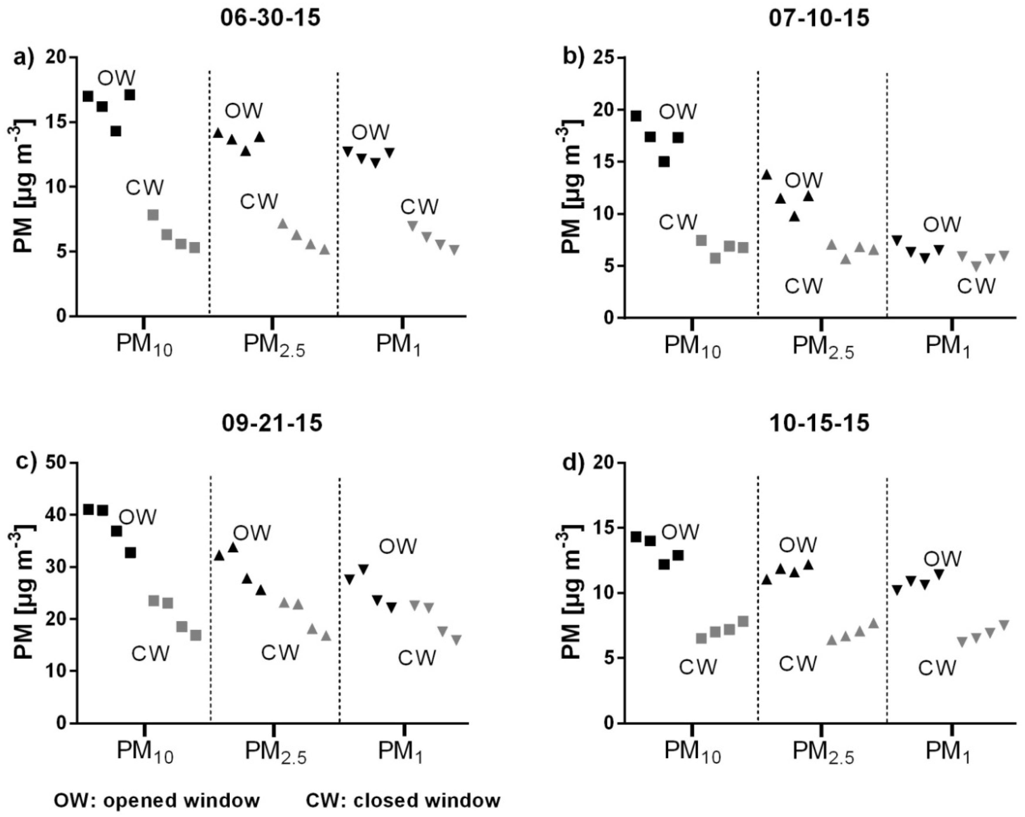
3.3. In-Cabin PM Concentration—Opened Window versus Closed Window

Medians for the PM10 concentration range between 12.2 µg m−3 and 41.1 µg m−3 (OW) and between 5.3 µg m−3 and 23.5 µg m−3 (CW). For PM2.5, medians range between 9.8 µg m−3 and 33.8 µg m−3 (OW) and between 5.2 µg m−3 and 23.2 µg m−3 (CW). Medians for PM1 range between 5.7 µg m−3 and 29.5 µg m−3 (OW) and between 4.9 µg m−3 and 22.6 µg m−3 (CW). Medians of the PM concentration of different particle fractions of four different days are shown in Figure 7.
On each of the four evaluation days, the concentrations of all fractions inside of the car were higher while driving with OW than while driving with CW. Differences in PM concentration could also be observed between the individual test rides (OW as well as CW rides) within a day. Both an increase and a decrease in concentration occurred. The u-test shows significantly high differences between driving with OW and with CW for all fractions with p-values <0.0001. The amount of PM reduction differs strongly between the single particle size fractions. In the coarse fraction (2.5–10 µm), there is a relative PM reduction between 87.9% and 97.4% (median: 96.9%) after closing the window. In the next finer fraction (1–2.5 µm), the PM reduction decreases to values between 77.9% and 88.2% (median: 82.3%). In the finest fraction (<1 µm), the PM reduction alternates very strongly between values from 13.0% to 52.0% (median: 31.1%). The absolute PM reduction varies between 1.5 µg m−3 and 7.8 µg m−3 (median: 4.2 µg m−3) for the coarse fraction, between 0.7 µg m−3 and 4.3 µg m−3 (median: 2.0 µg m−3) for the next finer fraction, and between 0.9 µg m−3 and 6.4 µg m−3 (median: 4.7 µg m−3) for the finest fraction. Thus, closing the window has a significant reducing impact on the PM concentrations in the car, especially on the coarser particles (Figure 8).

4. Discussion

4.1. Variations in the Local Particle Concentration and Size Distribution within the Urban Area

Outside PM concentration and particle size distribution has a significant effect to the concentration measured inside the cabin and is strongly dependent on the location. Even single point sources can lead to concentration shifts inside the cabin [29].
It becomes apparent that in-cabin PM concentrations of the PM2.5 and PM1 fraction are only changing slightly while driving through the city under OW conditions, with marginal higher values in the city center and on busy roads. These finer particles have a high residence time in the atmosphere and are widely and equally spread. Particles of those fractions can still be measured far away from their sources and therefore can also affect areas with a low primary PM emission within the city [30]. That leads to the comparatively steady in-cabin PM concentration.
Particles in this size range (PM2.5, PM1) typically originate from vehicle emissions, like abrasion of tires, brakes, and gear shifts, but also from combustion processes. Furthermore, particles from transformation processes of gaseous species and aged particles of other origins occur within this size range [1,30]. Although diesel cars in environmental zones, like in Frankfurt am Main, need to have particle filters and gasoline cars have modern catalytic converters, direct exhaust PM emissions can be measured. Most particles emitted by diesel engines are smaller than 1 µm and mainly appear in two main size ranges. Larger particles with a diameter up to 0.5 µm belong to the accumulation mode and mainly consist of solid material, such as carbon or metallic ash. The smaller particles with diameters under 50 nm belong to the nucleation mode and mainly comprise volatile material [31]. Most particles, especially from the accumulation mode, which partly are in the measuring range of the spectrometer (>0.25 µm), are eliminated by the particle filters. However, there is still a certain part of particles that is not eliminated, especially when the filter is not working probably [32].
In Figure 6a,b, examples for obvious PM sources as direct exhaust emissions are shown. There was probably a problem with the engine or the exhaust system in the car with the visible soot production, whereas behind older buses and heavy duty vehicles, generally high concentrations can be measured as well [21,33]. Also, cars with gasoline engines can emit particles in the measuring range of the spectrometer. Since controlled catalytic converters have been established in Germany since the late 1980s, PM concentrations of emissions of gasoline engines and their particle diameters are low [34,35]. However, especially modern cars with low CO2 emissions and direct injection engines emit high PM concentrations with higher particle diameters, which also can be measured by the spectrometer used in this campaign [36]. There were a lot more of those short-term concentration peaks in the size fraction smaller than 1 µm, which could not be linked to certain sources. It can be assumed that several of those peaks also reflect PM emissions from combustion processes of diesel or gasoline cars. The fact that a very high peak concentration for PM1 with a value of 122.9 µg m−3 was measured while standing at a stop light is an indication for such exhaust-related PM emissions.
In summary, the PM2.5 and PM1 signal seemed to be a combination of the urban background concentration, mainly of aged mixed aerosols, and the local emission peaks in areas with high traffic caused by abrasion processes and partly by direct exhaust emissions too. The PM fractions, PM2.5 and PM1, are only limited as being suitable as tracers for traffic emissions because of the relative high background level and its equal distribution. Chowdhury et al. already showed that in urban areas, direct emissions caused by traffic only play a minor role for the ambient PM2.5 concentration [37].
Background concentrations of the coarse particles (PMcoarse) while driving with an opened window was alternating stronger than the background concentration of the smaller fractions. The highest PM levels were reached in the city center, where plenty of short-term peaks can be observed. PMcoarse is mainly produced by abrasion of tires or brakes, raised dust, and resuspension in the wake of passing traffic [1]. These coarse particles are eliminated from the atmosphere quickly by depositing [38]. They can only be measured locally. For that reason, they show a strong alternating background signal with many significant short-term concentration peaks. Especially in busy streets, this background value was high in each ride.
Figure 6c,d are typical examples for sources of PMcoarse. The street sweeper as well as the garbage truck raise dust off the street while cleaning or while depositing garbage.
The PM10 signal, which includes the particles of all size categories (PM1, PM2.5, PMcoarse), shows a pattern of a rather constant concentration of the finer fractions (PM1, PM2.5) and also the impact of the strong concentration variations in the coarse fraction (PMcoarse).
While driving with a closed window, the patterns of PM10, PM2.5, and PM1 were very similar to each other. The reason for that is that almost exclusively, particles smaller than 1 µm were measured. In this case, the PM1 concentration matches the PM2.5 and the PM10 concentrations. Comparing the trend of the PM2.5 and the PM1 concentration from driving with OW and CW, the highest concentrations were measured in corresponding areas, which are mainly the busy roads in the city center. In contrast to driving with OW, the signal of PMcoarse neither shows a background nor a specific trend within the city while driving with CW. Nevertheless, there are some short-term concentration peaks irregularly distributed over the whole ride. They are probably not reflecting the outside concentration. More likely, they display processes inside the cabin, such as raising dust from the seats or the dashboard.

4.2. Comparability of Stationary versus Mobile Measured Particulate Matter

Positive correlations for certain particle fractions have shown that PMmean and PMAQMS correlate, even though the mobile measured local changing PM concentrations within a single round are not reflected by the static measured AQMS data. Also, PMdirect and PMAQMS concentrations correlate well although a single measured value of the AQMS represents the average concentrations of half an hour. In that time period, traffic may change significantly at the AQMS. Especially, the PM2.5 fraction can easily be correlated. That confirms that this fraction is equally distributed in the city and is independent of the location and the time of the measurement. These observations were made during the opened window and closed window rides.
In contrast, the mobile measured PMmean and PMdirect concentrations of the fraction, PMcoarse, are not reflected by the AQMS data, neither while driving with OW nor with CW. Particles of this fraction are distributed irregularly over the whole city, and concentration peaks in general only last for a short period of time. In this case, AQMS data from a single location has no informative value for the real drivers’ exposure.
The analysis of the PMcar/PMstation-quotients shows strong alternations between all rides. Developing a constant correction factor to approximate the in-cabin PM concentration from AQMS data is not reasonable.
While driving with OW, the in-cabin PM concentrations were approximately doubled if compared to corresponding values from the AQMS for all particle size fractions. That might be due to different reasons. Our mobile measuring device and thus also passengers in a car are normally much closer to the potential PM sources, like preceding vehicles or raised dust from the street, compared to the sample inlet from the AQMS installed at a height of 3.50 m, with a certain distance to the street [39,40]. Furthermore, the volume of the cabin is very limited so that PM can be accumulated and higher concentrations can be reached [41]. Different studies have already demonstrated that data from AQMS and the actual exposure in a car can differ significantly [18,29,41]. Kaur et al. has found that traffic participants are exposed to generally higher concentrations than data from AQMS would suggest [18]. Praml and Schierl even revealed a three to five times higher PM concentration inside the cabins of buses and trams in contrast to the data from an AQMS station near the road [29].
While driving with CW, concentrations from the mobile measurement and the AQMS are in the same range for PM10 and PM2.5. Particles of PMcoarse reach a much lower concentration in the cabin. So, closing the window and driving with AC on medium ventilation can probably partly reduce the in-cabin PM concentration.
Studies that prove whether in-cabin PM concentrations, generally, are higher than the direct ambient air are discussed controversially [22,42,43,44]. Putative conflicting results can partially be explained by different driving settings. Ventilation mode, traffic situation, and the type of car seem to be critical factors [45,46,47,48].
This study was performed in terms of modern mobility with an electric vehicle. It can be assumed that in vehicles, which themselves have very high PM emissions, even higher in-cabin concentrations can be measured.
For the evaluation, whether the achieved in-cabin PM concentrations have a potential harmful effect to health, limit values have to be set. Because official valid PM limit values are only defined for outside air, results of medical studies for in-cabin PM concentrations can be used for an assessment [49]. Riediker et al. revealed that the average PM2.5 concentration of 24 µg m−3 reached in the cabin during a shift of highway patrols on four subsequent days led to decreased lymphocytes and increased red blood cells, heart beat cycle length, and heart rate variability [50]. PM values of this magnitude were reached at the mobile OW measurement more often than the AQMS data suspected. Furthermore, high short-term in-cabin PM concentrations with a high medical relevance cannot be detected by the AQMS. The limited room of a cabin favors long-lasting high PM concentrations [41].
The data of the AQMS station can only, to a limited extent, approximate the actual PM exposure of a passenger. The daily shifting background concentration, which is reflected in the AQMS and in-cabin measurements, is mainly responsible for good correlations between AQMS and in-cabin PM concentration values. Meteorological variables, like wind speed or atmospheric stability, are the determining parameters in this case [51]. The daily traffic volume, which underlays high fluctuations, and the different point sources, which appear within one ride irregularly, are partly overlaid by this shifting background concentration. Despite good correlations between AQMS and in-cabin PM concentration values, absolute values strongly differ and thus, an exposure assessment including a medical risk assessment on the basis of AQMS data is highly uncertain.
Especially, high short-term in-cabin exposures cannot be captured by AQMS data and we conclude that mobile measurements are indispensable for monitoring them. Also, the particle size distribution of the PM exposure cannot be analyzed with AQMS data probably because there is no further differentiation within particle sizes smaller than 2.5 µm. The aerosol spectrometer used in our campaign is able to analyze and categories particles down to a size of 0.25 µm. This additional classification is of high medical importance because different particle sizes have different adverse health effects. Especially, airborne particles with aerodynamic diameters less than 1 µm have a high probability of deposition in the respiratory tract. Exacerbate respiratory diseases may be consequences. Small particles also lead to a higher burden of toxins. While absorbing those particles, negative respiratory health effects are possible [52,53,54].

4.3. Comparison of In-Cabin PM Exposure on Drivers between Rides with an Opened and Closed Window

When driving with CW and AC turned on, the PM concentration is significantly lower than while driving with an OW. Due to the filtering system and a smaller degree of air exchange, a decrease of the concentration can be reached. Jain and Apte et al. also showed that using AC in a car with CW can lead to lower concentrations while driving through urban areas [33,55]. Closing the window and using the AC also leads to a shift in the particle size distribution to particles with smaller diameters. The car filtering systems are rather suitable for reducing bigger particles. Smaller particles are not affected and not eliminated properly [44].
While driving through areas with a high PM pollution, it is sensible to close the window and use the AC. Thus, the total PM amount is reduced significantly. Although the potentially more harmful particles with smaller diameters are only reduced slightly, on days with a high pollution, also a significant absolute reduction in this size fraction can be reached.
Our test vehicle had a new pollen filter and was parked in an underground car park between the individual test rides. It is expected that the filter performance would decrease after a long run and permanent weather exposure. It must be ensured that vehicles are maintained regularly.
For further PM protection, using the internal recirculation mode from the AC or installing active charcoal filters may be an option [47,56].
Despite the short time frame of a measurement day, the PM concentration differences between the single OW rides and between the single CW rides can be explained by changes in external and internal conditions. Individual point sources along the roadside, such as raised dust or changes in wind speed, are examples of this. Small air turbulences, accumulation processes, or sedimentation can also lead to changes of in-cabin PM concentration.

4.4. Limitation of the Study

The PM measurements were carried out by a mobile aerosol spectrometer. Although more precise methods are available, they would not be suitable for mobile measurements. Particles with aerodynamic diameters below 0.25 µm cannot be detected. Since particles with diameters up to 0.1 µm still belong to the particulate matter fraction, a small proportion cannot be measured.
For the comparison of mobile measured data with PM data from stationary measurement, in-cabin concentrations were compared to the chronological fitting PM data of the AQMS. Since the highest resolution of the AQMS data is given for a 0.5 h mean value, slight deviations to the mobile measurement could not be avoided.

5. Conclusions

This study showed the importance of mobile measurements in the context of quantifications of in-cabin PM exposure. PM concentrations and PM size distributions were analyzed while driving through the city. Concentrations of smaller particles (PM2.5 and PM1) had a rather equal level in the city with slightly higher values in areas with a high traffic density. The concentration of coarse particles was rather dependent on single point sources and not distributed evenly over the whole city. Highest concentrations were reached in high-traffic areas. Several concentration peaks with characteristic particle sizes were linked to their sources. The PM10 concentration seemed to be the best indicator for traffic-based PM pollution. Smaller particles that show relatively constant background concentrations and emissions of combustion processes on the one hand and coarse particles, which are an indication for areas with a high traffic density in general, on the other hand are included in this particle size fraction.
Data of the AQMS can be used as an indication for the PM exposure to the passengers, but with comparatively low evidence. Especially, the in-cabin concentration while driving with OW would be underestimated and very high short-term concentration peaks cannot be identified. These concentrations measured in the car are of crucial medical relevance. By closing the window and using the AC, the in-cabin PM concentration was significantly reduced. Especially, coarse particles were efficiently eliminated. On the contrary, the elimination of PM with diameters smaller than 1 µm was modest.
It can be assumed that increased particulate matter pollution in urban areas with its health consequences will remain a serious problem in the future. All the more, it is important to consider different exposure scenarios in a differentiated way. Policymakers should also focus on indoor concentrations and, where appropriate, modify limit values.
A worthy extension of our campaign would be the use of aerosol spectrometers for in-depth investigation of the size distribution of ultrafine- and nanoparticles, which are of utmost importance for human health. In addition, a chemical analysis of this small-sized PM may further help to better understand potential health risks from traffic-borne air pollution.
Since, in many places, AQMS data is used for urban risk assessments, a study extension to other cities is reasonable. It is important that the geographical position of the AQMS within the city must be considered individually. Here, ensuring continuous data collection is essential. For a realistic measurement scenario, a representative route should be chosen.

Supplementary Materials

The following are available online at https://www.mdpi.com/1660-4601/15/12/2642/s1. Data set 1: PM data from the circular drive (mean values) and AQMS data. Data set 2: PM data from the circular drive (direct measurement) and AQMS data. Data set 3: PM data from the residental area. Data set 4:PM data from different point sources.

Author Contributions

Conceptualization, J.D. and D.A.G.; Data curation, J.D.; Formal analysis, J.D. and R.M.; Investigation, J.D.; Methodology, J.D.; Project administration, J.D.; Resources, D.A.G.; Software, C.S.; Supervision, J.D.; Validation, J.D., R.M. and D.A.G.; Visualization, J.D.; Writing—original draft, J.D.; Writing—review & editing, R.M., Markus Braun and D.A.G.

Funding

This research received no external funding.

Acknowledgments

The research presented here was undertaken as part and continuation of the Mobile Air Quality Study (MAQS). The authors thank the HLUG for the availability of air quality data from the regional network. Furthermore the authors like to thank the vehicle management of the Goethe-University Frankfurt am Main that provided the electric vehicle used in the study.

Conflicts of Interest

The authors declare no conflict of interest.

References

  1. Thorpe, A.; Harrison, R.M. Sources and properties of non-exhaust particulate matter from road traffic: A review. Sci. Total Environ. 2008, 400, 270–282. [Google Scholar] [CrossRef] [PubMed]
  2. Marcazzan, G.M.; Vaccaro, S.; Valli, G.; Vecchi, R. Characterisation of PM10 and PM2.5 particulate matter in the ambient air of Milan (Italy). Atmos. Environ. 2001, 35, 4639–4650. [Google Scholar] [CrossRef]
  3. Charron, A.; Harrison, R.M.; Quincey, P. What are the sources and conditions responsible for exceedences of the 24 h PM10 limit value (50 μgm−3) at a heavily trafficked London site? Atmos. Environ. 2007, 41, 1960–1975. [Google Scholar] [CrossRef]
  4. Colbeck, I. (Ed.) Aerosol Science: Technology and Applications; Wiley: Chichester, UK, 2014. [Google Scholar]
  5. Air Quality Expert Group. Particulate Matter in the United Kingdom; Defra: London, UK, 2005. [Google Scholar]
  6. EPA. Research on Health and Environmental Effects of Air Quality. 2017. Available online: https://www.epa.gov/air-research/research-health-and-environmental-effects-air-quality (accessed on 21 April 2017).
  7. Auchincloss, A.H.; Diez Roux, A.V.; Dvonch, J.T.; Brown, P.L.; Barr, R.G.; Daviglus, M.L.; Goff, D.C.; Kaufman, J.D.; O’Neill, M.S. Associations between recent exposure to ambient fine particulate matter and blood pressure in the Multi-ethnic Study of Atherosclerosis (MESA). Environ. Health Perspect. 2008, 116, 486–491. [Google Scholar] [CrossRef] [PubMed]
  8. Katsouyanni, K.; Touloumi, G.; Spix, C.; Schwartz, J.; Balducci, F.; Medina, S.; Rossi, G.; Wojtyniak, B.; Sunyer, J.; Bacharova, L.; et al. Short-term effects of ambient sulphur dioxide and particulate matter on mortality in 12 European cities: Results from time series data from the APHEA project. Air Pollution and Health: A European Approach. BMJ 1997, 314, 1658–1663. [Google Scholar] [CrossRef] [PubMed]
  9. Delfino, R.J.; Zeiger, R.S.; Seltzer, J.M.; Street, D.H. Symptoms in Pediatric Asthmatics and Air Pollution: Differences in Effects by Symptom Severity, Anti-Inflammatory Medication Use and Particulate Averaging Time. Environ. Health Perspect. 1998, 106, 751–761. [Google Scholar] [CrossRef] [PubMed]
  10. Michaels, R.A.; Kleinman, M.T. Incidence and Apparent Health Significance of Brief Airborne Particle Excursions. Aerosol Sci. Technol. 2000, 32, 93–105. [Google Scholar] [CrossRef] [Green Version]
  11. Pope, C.A.; Burnett, R.T.; Thun, M.J.; Calle, E.E.; Krewski, D.; Ito, K.; Thurston, G.D. Lung cancer, cardiopulmonary mortality, and long-term exposure to fine particulate air pollution. JAMA 2002, 287, 1132–1141. [Google Scholar] [CrossRef] [PubMed]
  12. Brook, R.D.; Rajagopalan, S.; Pope, C.A.; Brook, J.R.; Bhatnagar, A.; Diez-Roux, A.V.; Holguin, F.; Hong, Y.; Luepker, R.V.; Mittleman, M.A.; et al. Particulate matter air pollution and cardiovascular disease: An update to the scientific statement from the American Heart Association. Circulation 2010, 121, 2331–2378. [Google Scholar] [CrossRef] [PubMed]
  13. Dejmek, J.; Selevan, S.G.; Benes, I.; Solansky, I.; Sram, R.J. Fetal growth and maternal exposure to particulate matter during pregnancy. Environ. Health Perspect. 1999, 107, 475–480. [Google Scholar] [CrossRef] [PubMed]
  14. Creason, J.; Neas, L.; Walsh, D.; Williams, R.; Sheldon, L.; Liao, D.; Shy, C. Particulate matter and heart rate variability among elderly retirees: The Baltimore 1998 PM study. J. Expo. Anal. Environ. Epidemiol. 2001, 11, 116–122. [Google Scholar] [CrossRef] [PubMed]
  15. Liao, D.; Creason, J.; Shy, C.; Williams, R.; Watts, R.; Zweidinger, R. Daily Variation of Particulate Air Pollution and Poor Cardiac Autonomic Control in the Elderly. Environ. Health Perspect. 1999, 107, 521–525. [Google Scholar] [CrossRef] [PubMed]
  16. Williams, R.; Creason, J.; Zweidinger, R.; Watts, R.; Linda Sheldon Shy, C. Indoor, outdoor, and personal exposure monitoring of particulate air pollution: The Baltimore elderly epidemiology-exposure pilot study. Atmos. Environ. 2000, 34, 4193–4204. [Google Scholar] [CrossRef]
  17. Umweltbundesamt. Air Monitoring Networks: Station Database of the Environmental Agency. 2017. Available online: http://www.env-it.de/stationen/public/language.do;jsessionid=301985B5B53A47A60F18CE16DCEDC92E?language=en (accessed on 11 September 2017).
  18. Kaur, S.; Nieuwenhuijsen, M.J.; Colvile, R.N. Fine particulate matter and carbon monoxide exposure concentrations in urban street transport microenvironments. Atmos. Environ. 2007, 41, 4781–4810. [Google Scholar] [CrossRef]
  19. Uibel, S.; Scutaru, C.; Mueller, D.; Klingelhoefer, D.; Hoang, D.M.L.; Takemura, M.; Fischer, A.; Spallek, M.F.; Unger, V.; Quarcoo, D.; et al. Mobile air quality studies (MAQS) in inner cities: Particulate matter PM10 levels related to different vehicle driving modes and integration of data into a geographical information program. J. Occup. Med. Toxicol. 2012, 7, 20. [Google Scholar] [CrossRef] [PubMed]
  20. Groneberg, J.D.A.; Scutaru, C.; Lauks, M.; Takemura, M.; Fischer, T.C.; Kölzow, S.; van Mark, A.; Uibel, S.; Wagner, U.; Vitzthum, K.; et al. Mobile Air Quality Studies (MAQS)—An International Project; Universitätsbibliothek Johann Christian Senckenberg: Frankfurt am Main, Germany, 2010. [Google Scholar]
  21. Weijers, E. Variability of particulate matter concentrations along roads and motorways determined by a moving measurement unit. Atmos. Environ. 2004, 38, 2993–3002. [Google Scholar] [CrossRef] [Green Version]
  22. Gulliver, J.; Briggs, D.J. Personal exposure to particulate air pollution in transport microenvironments. Atmos. Environ. 2004, 38, 1–8. [Google Scholar] [CrossRef]
  23. MID. Mobilität in Deutschland 2008: Ergebnisbericht Struktur—Aufkommen—Emissionen—Trends; Infas, DLR: Bonn/Berlin, Germany, 2010. [Google Scholar]
  24. Krzyzanowski, M. Health Effects of Transport-Related Air Pollution: Summary for Policy Makers; WHO Regional Office for Europe: Copenhagen, Denmark, 2005. [Google Scholar]
  25. Wichmann, J.; Janssen, N.; Vanderzee, S.; Brunekreef, B. Traffic-related differences in indoor and personal absorption coefficient measurements in Amsterdam, the Netherlands. Atmos. Environ. 2005, 39, 7384–7392. [Google Scholar] [CrossRef]
  26. van Roosbroeck, S.; Hoek, G.; Meliefste, K.; Janssen, N.A.H.; Brunekreef, B. Validity of Residential Traffic Intensity as an Estimate of Long-Term Personal Exposure to Traffic-Related Air Pollution among Adults. Environ. Sci. Technol. 2008, 42, 1337–1344. [Google Scholar] [CrossRef] [PubMed]
  27. Zensus. Kreisfreie Städte und Landkreise nach Fläche und Bevölkerung auf Grundlage des ZENSUS 2011 und Bevölkerungsdichte; Statistisches Bundesamt: Wiesbaden, Germany, 2011.
  28. Bukowiecki, N.; Dommen, J.; Prévôt, A.; Richter, R.; Weingartner, E.; Baltensperger, U. A mobile pollutant measurement laboratory—Measuring gas phase and aerosol ambient concentrations with high spatial and temporal resolution. Atmos. Environ. 2002, 36, 5569–5579. [Google Scholar] [CrossRef]
  29. Praml, G.; Schierl, R. Dust exposure in Munich public transportation: A comprehensive 4-year survey in buses and trams. Int. Arch. Occup. Environ. Health 2000, 73, 209–214. [Google Scholar] [CrossRef] [PubMed]
  30. Gugamsetty, B. Source Characterization and Apportionment of PM10, PM2.5 and PM0.1 by Using Positive Matrix Factorization. Aerosol Air Qual. Res. 2012, 12, 491–496. [Google Scholar] [CrossRef]
  31. Kittelson, D.B.; Watts, W.F.; Johnson, J.P. Nanoparticle emissions on Minnesota highways. Atmos. Environ. 2004, 38, 9–19. [Google Scholar] [CrossRef]
  32. Fiebig, M.; Wiartalla, A.; Holderbaum, B.; Kiesow, S. Particulate emissions from diesel engines: Correlation between engine technology and emissions. J. Occup. Med. Toxicol. 2014, 9, 6. [Google Scholar] [CrossRef] [PubMed]
  33. Jain, S. Exposure to in-vehicle respirable particulate matter in passenger vehicles under different ventilation conditions and seasons. Sustain. Environ. Res. 2017, 27, 87–94. [Google Scholar] [CrossRef]
  34. Greenwood, S.J.; Coxon, J.E.; Biddulph, T.; Bennett, J. An Investigation to Determine the Exhaust Particulate Size Distributions for Diesel, Petrol, and Compressed Natural Gas Fuelled Vehicles. In An Investigation to Determine the Exhaust Particulate Size Distributions for Diesel, Petrol, and Compressed Natural Gas Fuelled Vehicles; SAE International400 Commonwealth Drive: Warrendale, PA, USA, 1996. [Google Scholar]
  35. Graskow, B.R.; Kittelson, D.B.; Ahmadi, M.R.; Morris, J.E. Exhaust Particulate Emissions from a Direct Injection Spark Ignition Engine. In Exhaust Particulate Emissions from a Direct Injection Spark Ignition Engine; SAE International400 Commonwealth Drive: Warrendale, PA, USA, 1999. [Google Scholar]
  36. Lv, G.; Song, C.; Pan, S.; Gao, J.; Cao, X. Comparison of number, surface area and volume distributions of particles emitted from a multipoint port fuel injection car and a gasoline direct injection car. Atmos. Pollut. Res. 2014, 5, 753–758. [Google Scholar] [CrossRef]
  37. Chowdhury, Z.; Zheng, M.; Schauer, J.J.; Sheesley, R.J.; Salmon, L.G.; Cass, G.R.; Russell, A.G. Speciation of ambient fine organic carbon particles and source apportionment of PM 2.5 in Indian cities. J. Geophys. Res. 2007, 112, 111. [Google Scholar] [CrossRef]
  38. BAFU. Feinstaub PM 10: Fragen und Antworten zu Eigenschaften, Emissionen, Immissionen, Auswirkungen und Massnahmen; Budesamt für Umwelt, Wald und Landwirtschaft: Bern, Switzerland, 2006. [Google Scholar]
  39. Gee, I.L.; Raper, D.W. Commuter exposure to respirable particles inside buses and by bicycle. Sci. Total Environ. 1999, 235, 403–405. [Google Scholar] [CrossRef]
  40. Hessiches Landesamt für Naturschutz, Umwelt und Geologie: Air monitoring network Hessen. 2018. Available online: https://www.hlnug.de/fileadmin/scripts/recherche/info/FrankfurtFriedbergerLandstr.pdf (accessed on 24 November 2018).
  41. Geiss, O. Exposure to Particulate Matter in Vehicle Cabins of Private Cars. Aerosol Air Qual. Res. 2010, 10, 581–588. [Google Scholar] [CrossRef]
  42. Geiss, O.; Tirendi, S.; Barrero-Moreno, J.; Kotzias, D. Investigation of volatile organic compounds and phthalates present in the cabin air of used private cars. Environ. Int. 2009, 35, 1188–1195. [Google Scholar] [CrossRef] [PubMed]
  43. Boogaard, H.; Borgman, F.; Kamminga, J.; Hoek, G. Exposure to ultrafine and fine particles and noise during cycling and driving in 11 Dutch cities. Atmos. Environ. 2009, 43, 4234–4242. [Google Scholar] [CrossRef]
  44. Briggs, D.J.; de Hoogh, K.; Morris, C.; Gulliver, J. Effects of travel mode on exposures to particulate air pollution. Environ. Int. 2008, 34, 12–22. [Google Scholar] [CrossRef] [PubMed]
  45. Van Wijnen, J.H.; Verhoeff, A.P.; Jans, H.W.; van Bruggen, M. The exposure of cyclists, car drivers and pedestrians to traffic-related air pollutants. Int. Arch. Occup. Environ. Health 1995, 67, 187–193. [Google Scholar] [CrossRef] [PubMed]
  46. Kingham, S.; Meaton, J.; Sheard, A.; Lawrenson, O. Assessment of exposure to traffic-related fumes during the journey to work. Transp. Res. Part D Transp. Environ. 1998, 3, 271–274. [Google Scholar] [CrossRef]
  47. Tartakovsky, L.; Baibikov, V.; Czerwinski, J.; Gutman, M.; Kasper, M.; Popescu, D.; Mark, V.; Zvirin, Y. In-vehicle particle air pollution and its mitigation. Atmos. Environ. 2013, 64, 320–328. [Google Scholar] [CrossRef]
  48. Alm, S.; Jantunen, M.J.; Vartiainen, M. Urban commuter exposure to particle matter and carbon monoxide inside an automobile. J. Expo. Anal. Environ. Epidemiol. 1999, 9, 237–244. [Google Scholar] [CrossRef] [PubMed] [Green Version]
  49. European Union. Official Journal of the European Union L 152, 11.06.2008: Directive 2008/50/EC of the European Parliament and of the Council of 21 May 2008 on Ambient Air Quality and Cleaner Air for Europe; Publications Office of the European Union: Luxembourg, 2008. [Google Scholar]
  50. Riediker, M.; Devlin, R.B.; Griggs, T.R.; Herbst, M.C.; Bromberg, P.A.; Williams, R.W.; Cascio, W.E. Cardiovascular effects in patrol officers are associated with fine particulate matter from brake wear and engine emissions. Part. Fibre Toxicol. 2004, 1, 2. [Google Scholar] [CrossRef] [PubMed] [Green Version]
  51. Gualtieri, G.; Toscano, P.; Crisci, A.; Di Lonardo, S.; Tartaglia, M.; Vagnoli, C.; Zaldei, A.; Gioli, B. Influence of road traffic, residential heating and meteorological conditions on PM10 concentrations during air pollution critical episodes. Environ. Sci. Pollut. Res. Int. 2015, 22, 19027–19038. [Google Scholar] [CrossRef] [PubMed]
  52. Dockery, D.W.; Pope, C.A.; Xu, X.; Spengler, J.D.; Ware, J.H.; Fay, M.E.; Ferris, B.G.; Speizer, F. An association between air pollution and mortality in six U.S. cities. N. Engl. J. Med. 1993, 329, 1753–1759. [Google Scholar] [CrossRef] [PubMed]
  53. Pope, C.A.; Thun, M.J.; Namboodiri, M.M.; Dockery, D.W.; Evans, J.S.; Speizer, F.E.; Heath, C.W., Jr. Particulate air pollution as a predictor of mortality in a prospective study of U.S. adults. Am. J. Respir. Crit. Care Med. 1995, 151 Pt 1, 669–674. [Google Scholar] [CrossRef]
  54. Miller, F.J.; Gardner, D.E.; Graham, J.A.; Lee, R.E.; Wilson, W.E.; Bachmann, J.D. Size Considerations for Establishing a Standard for Inhalable Particles. J. Air Pollut. Control Assoc. 1979, 29, 610–615. [Google Scholar] [CrossRef] [Green Version]
  55. Apte, J.S.; Kirchstetter, T.W.; Reich, A.H.; Deshpande, S.J.; Kaushik, G.; Chel, A.; Marshall, J.D.; Nazaroff, W.W. Concentrations of fine, ultrafine, and black carbon particles in auto-rickshaws in New Delhi, India. Atmos. Environ. 2011, 45, 4470–4480. [Google Scholar] [CrossRef]
  56. Muala, A.; Sehlstedt, M.; Bion, A.; Österlund, C.; Bosson, J.A.; Behndig, A.F.; Pourazar, J.; Bucht, A.; Boman, C.; Mudway, I.S.; et al. Assessment of the capacity of vehicle cabin air inlet filters to reduce diesel exhaust-induced symptoms in human volunteers. Environ. Health 2014, 13, 16. [Google Scholar] [CrossRef] [PubMed] [Green Version]
Figure 1. kml file with the local in-cabin particulate matter (PM) concentration measured while driving through Frankfurt am Main. Turquoise line: Location-dependent PM concentration. Geographical picture by Google Earth.
Ijerph 15 02642 g001
Figure 2. Course 1: Circular drive through Frankurt am Main passing the air quality monitoring stations (AQMS) “Friedberger Landstraße”. Red line: Driving route, yellow marks: Street names and places, green mark: Air quality monitoring station. Geographical picture by Google Earth.
Ijerph 15 02642 g002
Figure 3. Course 2: Circular drive through a residential area in Frankfurkt-Eschersheim. Red line: Driving route, yellow line: Main roads. Geographical picture by Google Earth.
Ijerph 15 02642 g003
Figure 4. Representative short-term concentration peaks measured with an opened window on 10-20-15. (a) At noon, (b) in the afternoon.
Ijerph 15 02642 g004
Figure 5. Representative in-cabin PM concentrations with corresponding background concentrations for PM10, PM2.5, and PMcoarse on 01-06-16. (ac) Measured while driving with an opened window; (df) measured while driving with a closed window. Geographical positions are marked by the numbers, 1–6.
Ijerph 15 02642 g005
Figure 6. Different PM sources with the corresponding particle size spectrum. (a) A car with soot production, (b) a bus, (c) a garbage truck, (d) a street sweeper (see also Supplementary Material 4).
Ijerph 15 02642 g006
Figure 7. Medians of in-cabin PM10, PM2.5, and PM1 concentrations measured with an opened and closed window. (a) On 06-30-15, (b) on 01-10-15, (c) on 09-21-15, (d) on 10-15-15 (see also Supplementary Material 3).
Ijerph 15 02642 g007
Figure 8. In-cabin PM concentrations and particle size distributions measured with an opened and closed window. (a) On 06-30-15, (b) on 07-10-15, (c) on 09-21-15, (d) on 10-15-15.
Ijerph 15 02642 g008
Table 1. Test rides on the circular drive through Frankfurt am Main.
(a)(b)
OWCWOWCW
DateTimeDateTimeDateTimeDateTime
05-22-1511:59–12:3905-22-1511:11–11:5205-22-1512:2605-22-1511:36
05-22-1514:26–15:0905-22-1513:42–14:2305-22-1514:5305-22-1514:07
05-29-1512:42–13:1805-29-1512:03–12:3905-29-1513:0505-29-1512:25
05-29-1515:50–16:3905-29-1515:00–15:4505-29-1516:1805-29-1515:22
10-15-1514:57–15:3210-20-1511:20–11:5410-15-1515:1710-20-1511:40
10-20-1510:42–11:1410-20-1514:50–15:2310-20-1510:5910-20-1515:08
10-20-1511:57–12:3212-01-1511:56–12:3210-20-1512:1712-01-1513:17
10-20-1514:09–14:4512-01-1517:36–18:1310-20-1514:3112-01-1518:58
12-01-1511:16–11:5112-02-1515:09–15:5012-01-1512:3712-02-1516:31
12-01-1516:47–17:3201-06-1615:38–16:1212-01-1518:1101-06-1615:59
12-02-1509:26–10:0001-07-1615:55–15:2712-02-1510:4701-07-1611:48
01-06-1614:55–15:3301-13-1618:17–18:5701-06-1612:4701-07-1615:13
01-07-1614:17–14:50 01-06-1615:1601-13-1614:52
01-13-1617:31–18:10 01-07-1614:3501-13-1619:41
01-13-1617:52
(a) Dates with the time and duration of the certain rounds; (b) dates and the point of time when the air quality monitoring stations (AQMS) “Friedberger Landstraße” was passed by the car; OW: Opened window; CW: Closed window.
Table 2. Dates and time frames of the test rides through the residential area in Frankfurt-Eschersheim.
Time Time
DateOWCWDateOWCW
06-30-1516:21–16:3116:34–16:4409-21-1510:55–11:0411:07–11:17
16:46–16:5616:59–17:09 11:18–11:2811:31–11:41
17:10–17:2017:24–17:33 11:42–11:5211:55–12:05
17:34–17:4417:48–17:58 12:07–12:1712:20–12:32
07-10-1510:52–11:0211:05–11:1510-15-1511:48–11:5712:00–12:09
11:28–11:3811:41–11:50 12:10–12:1912:24–12:34
11:53–12:0212:05–12:15 12:35–12:4512:48–12:57
12:23–12:3312:36–12:46 12:58–13:0813:11–13:20
OW: Opened window; CW: Closed window.
Table 3. Minimum and maximum concentrations for different PM fractions and AQMS data.
In-Cabin [µg m−3]PMAQMS [µg m−3]
MinMaxMinMax
OWPMmeanPM1017.163.76.435.7
PM2.512.943.23.126.6
PM110.639.5--
PMcoarse3.621.62.19.0
PMdirectPM1018.175.76.436.7
PM2.513.562.73.627.3
PM111.556.7--
PMcoarse1.721.71.99.4
CWPMmeanPM104.927.56.333.5
PM2.54.526.43.424.6
PM14.225.9--
PMcoarse0.21.92.08.9
PMdirectPM105.326.55.533.5
PM2.55.126.45.024.6
PM14.925.8--
PMcoarse0.02.50.58.9
Minimum and maximum in-cabin concentrations for the fractions PM10, PM2.5, PM1, and PMcoarse and the data of the AQMS measured at approximately the same point of time (see also Supplementary Material 1 and 2). OW: Opened window; CW: Closed window.
Table 4. Correlation coefficients for in-cabin PM concentrations and PM concentrations from the AQMS.
PMmean vs. PMAQMSPMdirect vs. PMAQMS
Spearmanp-ValueSpearmanp-Value
OWPM100.88<0.0010.670.008
PM2.50.93<0.0010.820.001
PMcoarse0.290.31−0.210.46
CWPM100.810.0020.780.001
PM2.50.85<0.0010.88<0.001
PMcoarse−0.140.67−0.210.47
OW: Opened window; CW: Closed window.
Table 5. Mean PMmean/PMAQMS-and PMdirect/PMAQMS-quotients of all rides on the circular drive.
PMmean/PMAQMS
(Means of All Rides)
PMdirect/PMAQMS
(Means of All Rides)
OWPM102.2 (CV: 0.29)2.2 (CV: 0.46)
PM2.52.5 (CV: 0.38)2.7 (CV: 0.43)
PMcoarse2.0 (CV: 0.68)1.7 (CV: 0.80)
CWPM101.0 (CV: 0.28)0.9 (CV: 0.20)
PM2.51.4 (CV: 0.26)1.3 (CV: 0.21)
PMcoarse0.2 (CV: 0.82)0.1 (CV: 1.23)
OW: Opened window; CW: Closed window; CV: Coefficient of variation.

