How Outdoor Trees Affect Indoor Particulate Matter Dispersion: CFD Simulations in a Naturally Ventilated Auditorium

Abstract

This study used computational fluid dynamics (CFD) models, coupling with a standard k-ε model based on the Reynolds-averaged Navier-Stokes (RANS) approach and a revised generalized drift flux model, to investigate effects of outdoor trees on indoor PM_1.0, PM_2.5, and PM₁₀ dispersion in a naturally ventilated auditorium. Crown volume coverage (CVC) was introduced to quantify outdoor trees. Simulations were performed on various CVCs, oncoming wind velocities and window opening sizes (wall porosities were 3.5 and 7.0%, respectively, for half and fully opened windows). The results were as follows: (1) A vortex formed inside the auditorium in the baseline scenario, and the airflow recirculation created a well-mixed zone with little variation in particle concentrations. There was a noticeable decrease in indoor PM₁₀ with the increasing distance from the inlet boundary due to turbulent diffusion. (2) Assuming that pollution sources were diluted through the inlet, average indoor particle concentrations rose exponentially with increasing oncoming wind speed. PM₁₀ changed most significantly due to turbulent diffusion and surface deposition reduction intensified by the increased wind velocity. (3) Increasing the window opening improved indoor cross-ventilation, thus reducing indoor particle concentrations. (4) When 2.87 m³/m² ≤ CVC ≤ 4.73 m³/m², indoor PM_2.5 could meet requirements of the World Health Organization’s air quality guidelines (IT-3) for 24-hour mean concentrations; and (5) average indoor particle concentrations had positive correlations with natural ventilation rates (R² = 0.9085, 0.961, 0.9683 for PM_1.0, PM_2.5, and PM₁₀, respectively, when the wall porosity was 3.5%; R² = 0.9158, 0.9734, 0.976 for PM_1.0, PM_2.5, and PM₁₀, respectively, when the wall porosity was 7.0%).

1. Introduction

Rapid urbanization, urban transportation, factory production and domestic biomass combustion have caused a dramatic decline in the quality of urban environments [1,2]. Atmospheric particles such as PM_1.0, PM_2.5 and PM₁₀ have turned into the most intractable problems of urban air pollution. Epidemiological studies have demonstrated that atmospheric particles are associated with malignancies, respiratory and cardiovascular diseases [3,4,5,6]. As most residents spend 85–90% of their time indoors, indoor air quality is closely related to human health. Therefore, understanding relationships between indoor and outdoor air pollution is critical to better characterize ambient particulate matter exposure and health effects [7,8].

It is well known that vegetation, especially trees, decreases atmospheric particles by capture, filtering, precipitation and turbulent diffusivity [9]. Tree species, canopy porosity, and leaf area density all affect atmospheric particles dispersion [10]. These effects have been recently quantified in wind tunnel tests and experimental studies on deposition velocities and capture efficiency of various trees [11,12,13,14,15]. Relative experimental studies were performed using mass subtraction [16,17], membrane filters [18,19,20,21], the elution-weighed approaches combining particle size analysis [22,23,24,25,26,27], and other direct determination methods [28,29,30]. These studies have largely focused on different particle size distributions of foliage among tree species [31,32], and variation in the particle size distribution on foliage with different dust retention durations [33]. Additionally, the deposition velocities of particulate matter were comparatively analyzed among a variety of trees in numerical simulations [13,34]. The impacts of trees on pollutants are frequently estimated using three-dimensional models, allowing the aerodynamics and deposition effects to be quantitatively calculated [35,36,37,38,39,40,41,42,43,44,45].

Natural ventilation of indoor airflow and cooling is based on outside air movement and pressure differences without mechanical assistance. Previous studies in European cities have shown that using natural ventilation, building energy can be reduced by 40–50% [46,47]. Nevertheless, few studies have examined how to improve indoor air quality through natural ventilation [48]. As concern for relationships between indoor and outdoor air quality has grown, so has the need for indoor and outdoor aerosol measurement [49]. Yet, some research has reported that improper measurement of natural ventilation may aggravate air quality, promoting the need for better indoor air quality measurement [50,51]. Indoor-to-outdoor (I/O) particle concentration ratios, permeability coefficient and other factors have been found to best reflect relationships between indoor and outdoor suspended particulates [52,53,54,55]. Additionally, indoor/outdoor PM_2.5 has shown a high correlation when there is no obvious indoor particle source [56,57]. Although the impact of outdoor meteorology on indoor particles in naturally ventilated classrooms has been investigated [58], I/O ratios reported have ranged widely from 0 to 5. This is perhaps because the spatial distribution of particles changes noticeably in built environments owing to a range of environmental conditions, particle sizes, building envelopes, greenspace layout and indoor pollution sources [59]. It is clearly difficult to fully understand the links between outdoor and indoor air quality simply based on the I/O ratio.

Numerous experimental studies, wind tunnel experiments and numerical simulations have suggested that plants are effective for abating atmospheric particles. Indoor particulate matter typically originates from outdoor spaces and building ventilation has significant impacts on indoor air pollution [60]. So far, a significant contribution has been made by Tong et al. in uncovering the impact of traffic-related air pollution on indoor air quality of a naturally ventilated building with realistic building characteristics and construction practices, where conditions with a complex internal zone layout were discussed [61]. However, few studies have focused on effects of outdoor trees on indoor/outdoor particles transportation. This study highlights the research gap relating outdoor tree planting on indoor particle concentration distributions. In this aspect, a key issue is to determine how to reduce particulate pollutant transportation from outdoors to indoors by optimizing tree planting and improving natural ventilation.

To fill this research gap, this study used computational fluid dynamics (CFD) models, integrating a standard k-ε model based on Reynolds-averaged Navier-Stokes (RANS) approach and a revised generalized drift flux model to predict the spatial relationship between indoor and outdoor pollutants via natural ventilation in a generalized auditorium. Our principle objective is to quantify the impact of outdoor trees on indoor/outdoor relationships of PM_1.0, PM_2.5 and PM₁₀ concentration distributions with different oncoming wind velocities and window opening sizes. The simulations were organized as follows: First, we described the CFD-based airflow and particle diffusion models. Second, the CFD models were validated by wind tunnel tests and a model chamber with a Phased-array Doppler Anemometry (PDA) experiment. Finally, we evaluated the impact of various parameters on indoor air quality through a series of quantitative simulations.

2. Methodology

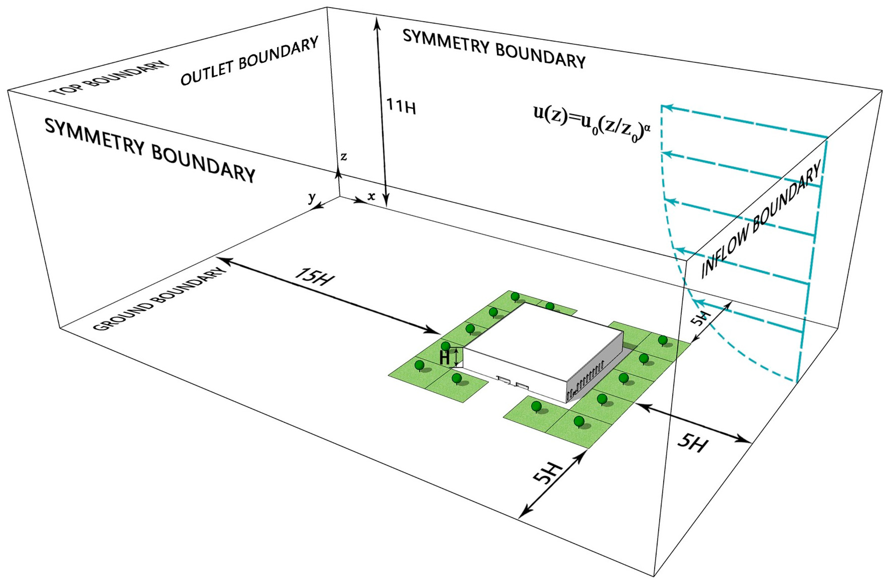
2.1. Simulation Model

In this study, we reproduced airflow and particle diffusion in an idealized auditorium and simulated conditions using three-dimensional steady-state isothermal flow field models. CFD simulations were aligned with the COST Action 732, including choices of target variables, approximation equations, geometrical representation of obstacles, computational domain, boundary conditions, initial data, computational grid, numerical approximations, and iterative convergence criteria [62]. The Reynolds-averaged Navier-Stokes (RANS) model, consisting of the k-ε Murakami-Mochida-Kondo (MMK) closure scheme, was used. This model was modified based on the standard k-ε model that could better represent airflow fields around buildings. The Semi-Implicit Method for Pressure-Linked Equations (SIMPLE) algorithm with the Quadratic Upstream Interpolation for Convective Kinematics (QUICK) discretization scheme was applied to all governing equations. The scaled iterative convergence criteria for all parameters in simulations were set to 10⁻⁶. Simulations were run on an i7 2.67 GHz processor (Intel, Santa Clara, CA, USA). The Parabolic Hyperbolic or Elliptic Numerical Integration Code Series (CHAM, London, UK, Edition: 2009) program was used to operate solutions.

In the airflow model, vegetation is parameterized as a porous medium. For calculation efficiency, tree branches and trunks are approximated as foliage and crowns, so that tree canopies (including branches and trunks) are modeled as a whole [63]. From the perspective of aerodynamics, trees reduce air velocity by applying resistance and pressure. Therefore, the resistance was taken into account based on momentum equations to simulate the effects of trees on turbulent flow fields. For extra sources of turbulent flow, the turbulent flow formation on tree canopies and its dissipation were also accounted for. Model equations are as:

Continuity equation:

$$\frac{\partial \langle u_i\rangle }{\partial x_i}=0$$

(1)

where u_i is spatial mean velocity (m/s), and x_i is spatial coordinate.

Momentum equation:

$$\frac{\partial \langle u_i\rangle }{\partial t}+\langle u_j\rangle \frac{\partial \langle u_i\rangle }{\partial x_j}=-\frac{1}{\rho }\frac{\partial \langle P\rangle }{\partial x_i}+\frac{\partial }{\partial x_j}\left({\nu }_{eff}\frac{\partial \langle u_i\rangle }{\partial x_j}\right)+F_d$$

(2)

where P is pressure (Pa); ρ is air density (kg/m³); F_d is an extra source of resistance on tree canopies; v_eff is effective viscosity (Ns/m²), which is calculated as:

$${\nu }_{eff}=\nu +{\nu }_t=\nu +c_{\mu }\frac{k^2}{\epsilon }$$

(3)

where k is turbulent kinetic energy (Nm); ε is dissipation rate (m/s); v_t is turbulent viscosity (Ns/m²); and c_μ is an empirical coefficient (set to 0.09) [64].

Based on conventional parameterization of plant-airflow interactions, F_d is expressed as:

$$F_d=-\frac{1}{2}{C}_d\eta a{u}_{i}S$$

(4)

$$S={\left({\displaystyle \sum {\langle u_i\rangle }^2}\right)}^{0.5}$$

(5)

where S is mean wind velocity (m/s); C_d is a drag coefficient for tree canopies. The drag coefficient for trees is estimated as 0.1 ≤ C_d ≤ 0.3 [65]. In this study, C_d is set to 0.2; α is leaf area density (m²/m³), and ηα is the projected area of foliage on the plane perpendicular to the prevailing wind direction (m²).

To model turbulence interactions between tree canopies and fluid (air), the kinetic turbulence equation is expressed as:

$$\frac{\partial k}{\partial t}+\langle u_j\rangle \frac{\partial k}{\partial x_j}=\frac{\partial }{\partial x_i}\left(\frac{{\nu }_t}{{\sigma }_k}\frac{\partial k}{\partial x_i}\right)+{\nu }_t\left(\frac{\partial \langle u_i\rangle }{\partial x_j}+\frac{\partial \langle u_j\rangle }{\partial x_i}\right)\frac{\partial \langle u_i\rangle }{\partial x_j}-\epsilon +P_k+L_k$$

(6)

P_k and L_k are extra source terms of the equation, and expressed as:

$$P_k=\frac{1}{2}{C}_d\eta a{S}^3$$

(7)

$$L_k=-2C_d\eta aSk$$

(8)

Likewise, while considering impacts of tree canopies, the dissipation rate of kinetic energy is calculated as:

$$\frac{\partial \epsilon }{\partial t}+\langle u_j\rangle \frac{\partial \epsilon }{\partial x_j}=\frac{\partial }{\partial x_i}\left(\frac{{\nu }_t}{{\sigma }_{\epsilon }}\frac{\partial \epsilon }{\partial x_i}\right)+C_{\epsilon 1}\frac{\epsilon }{k}{\nu }_t\left(\frac{\partial \langle u_i\rangle }{\partial x_j}+\frac{\partial \langle u_j\rangle }{\partial x_i}\right)\frac{\partial \langle u_i\rangle }{\partial x_j}-C_{\epsilon 2}\frac{{\epsilon }^2}{k}+P_{\epsilon }+L_{\epsilon }$$

(9)

P_ε and L_ε are extra source terms of the above equation, and determined as follows:

$$P_{\epsilon }=\frac{\epsilon }{k}{C}_{p\epsilon 1}{C}_d\eta a{S}^3$$

(10)

$$L_{\epsilon }=-4C_{p\epsilon 2}{C}_d\eta aS\epsilon$$

(11)

where σ_k, σ_ε, C_ε1 and C_ε2 are empirical constants, equal to 1.0, 1.3, 1.44, and 1.92, respectively. The comparisons between field data and simulation results suggest that C_pε1 and C_pε2 are 1.8 and 0.6, respectively [66].

Foliage reduces atmospheric particles largely by deposition [67]. In Eulerian models, particles are deemed continuums in solving conservation equations between mass and molar concentration. These models are widely used for their accuracy and efficiency. The revised generalized drift flux model, which is a type of revised Eulerian model, takes into account the slippage between particles and the fluid (air). In the model, plants intensify particle deposition via turbulent diffusion. Plants also absorb particles, some of which may re-suspend over foliage [11]. To accommodate these, the deposition and resuspended effects of plants on particulate matter are conveyed through extra terms S_sink and S_resuspension. In this way, the revised generalized drift flux model can simulate an actual built environment comprehensively and accurately [68,69]. It is expressed as:

$$\frac{\partial \left[\left(V_j+V_{slip,j}\right)C\right]}{\partial x_j}=\frac{\partial }{\partial x_j}\left[{\epsilon }_p\frac{\partial C}{\partial x_j}\right]+S_c-S_{\sin k}+S_{resuspension}$$

(12)

The slippage velocity of particles (V_slip) is defined by gravity, thermal force by the thermophoresis effect, particle fluctuation due to turbulence and particle acceleration [68], and is calculated as:

$$V_{slip,j}={\tau }_p{g}_j+{\tau }_p{\displaystyle \sum F_j}+\frac{{\tau }_p}{C}{S}_{mj}-\frac{{\tau }_p}{C}\frac{\partial \left(V_{pj}{V}_{pi}C\right)}{\partial x_i}$$

(13)

$$S_{mj}=\frac{\partial }{\partial x_i}\left[{\epsilon }_{p}C\left(\frac{\partial V_{pj}}{\partial x_i}+\frac{\partial V_{pi}}{\partial x_j}\right)\right]+\frac{\partial }{\partial x_i}\left[{\epsilon }_p\left(V_{pi}\frac{\partial C}{\partial x_j}+V_{pj}\frac{\partial C}{\partial x_i}\right)\right]$$

(14)

$${\tau }_p=\frac{C_c{\rho }_p{d}_p^2}{18\mu }$$

(15)

The effect of tree canopies on absorbing atmospheric particles is dependent upon their leaf area densities (LADs), deposition velocities and particulate matter concentrations, conveyed as follows:

S_sink= α(z) × V_d × C

(16)

The resuspension of particulate matter, as a term of volume source, is described as:

S_resuspension = S_sink × P_resuspension

(17)

P_resuspension = −0.00041v² + 0.017v − 0.0016

(18)

Since grass is depicted as a plane in this model, the leaf area density of grass is expressed as [40]:

LAD_grass = S/V × LAI_grass

(19)

where V_j and V_slip,j are the respective mean fluid (air) velocity and gravitational settling velocity of particles in direction j (m/s). C is particle concentration at the inlet (μg/m³); ε_p is turbulent diffusivity (m²/s), and can be simplified to 1 [68]. S_c is the formation rate of particle sources (kg/m³s). S_sink is the mass of particle absorbed by vegetation per cubic meter within a unit of time (μg/m³); S_resuspension is the secondary pollutant generated by foliage per cubic meter within a unit of time [70]; V_d is particle deposition velocity on foliage (m/s); P_resuspension is the percentage of resuspended particles; v is the magnitude of air velocity (m/s), and α is LAD (m²/m³). V_pj and V_pi are velocities of particles in directions j and i (m/s), respectively. τ_p is the relaxation time of a particle; g_j is the gravitational acceleration in direction j (m/s²); ΣF_j is the resultant force exerted upon the particle (m/s²); S_mj is the momentum source of particle in direction j (kg/(m² s²); μ is the molecular kinematic viscosity of air(Ns/m²); ρ_p is the density of atmospheric particles (kg/m³); and d_p is the particle diameter (m); C_c is the Cunningham factor induced by slippage. S is the grass surface area (m²), V is grass volume within the computational domain (m³), and LAI_grass is the leaf area index of grass (m³/m³).

2.2. Model Validation

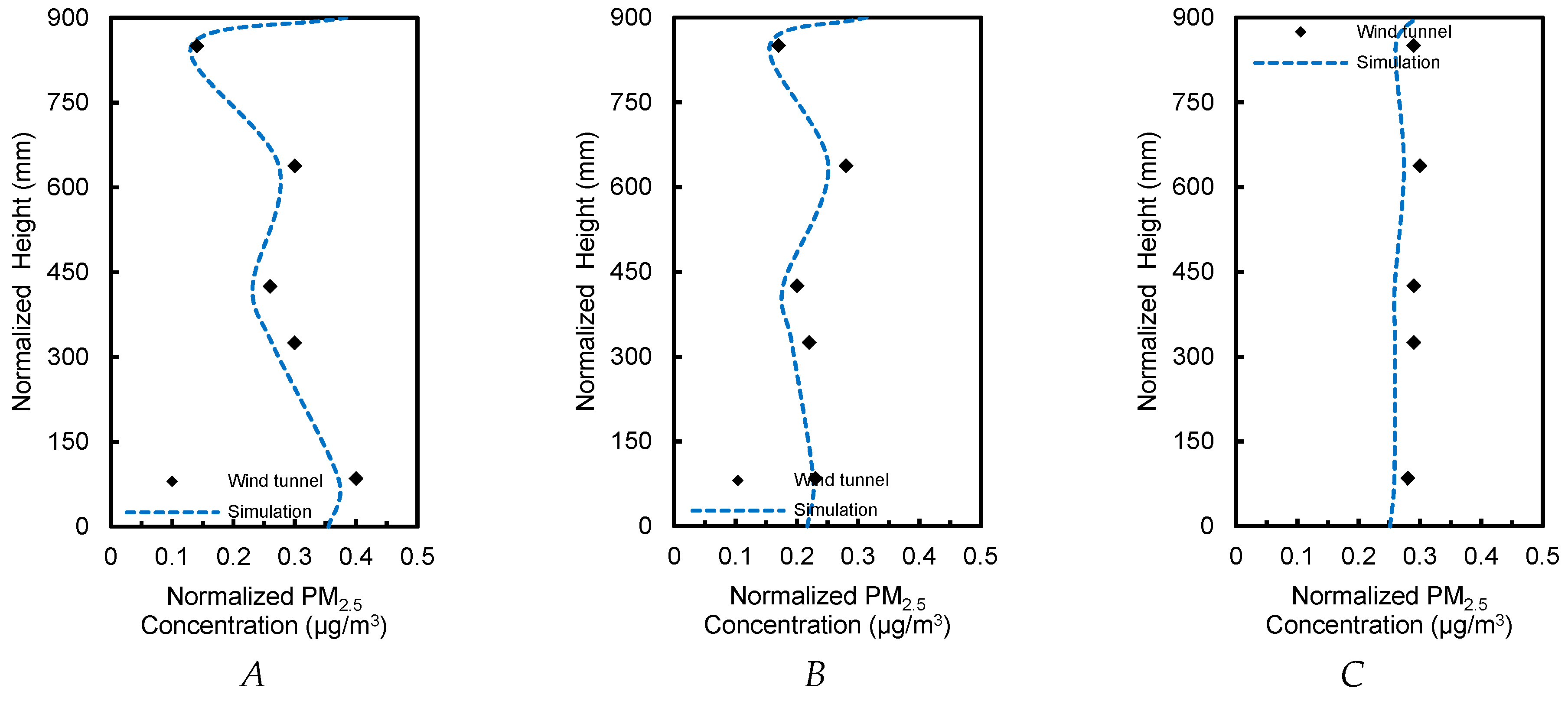
2.2.1. Aerodynamic and Deposition Effects of Trees around Buildings

Ji et al. studied the impact of trees on PM_2.5 distribution around buildings using wind tunnel experiments [71]. In their tests, buildings and trees were arranged perpendicularly to the oncoming wind at a scale of 1:20 with dimensions of 18L × 12W × 3.5H. The dimension of a single building is 1.5 mL × 0.75 mW × 0.85 mH. To test the impact of trees on airflow and PM_2.5 distribution more accurately, fresh cypress branches and leaves were used. Cypress was fully leached to remove dust. The crown diameter and tree height were 0.23 and 0.35 m, respectively. A “line source” of particles was released from the inlet with an oncoming wind velocity of 4.5 m/s in the wind tunnel. The airflow field and PM_2.5 concentration distributions around buildings at the pedestrian height (85 mm), mid-canopy height (325 mm), mid-building height (425 mm), three-quarters of the building height (637.5 mm), and the top of the building (850 mm) in the vertical plane were investigated.

The simulation model was built based on the size of buildings and trees (Figure 1). Following research guidelines [62,72], the distance between the windward side of front-row buildings and the inflow boundary was set to 5H, while the distance between the leeward side of back-row buildings and the outflow boundary was 15H. The distance between the left/right symmetric boundary and the target area was 5H, and the distance from the ground to the top boundary was 11H. The oncoming wind at the inlet is gradient wind and is conveyed by the equation:

$$u\left(z\right)=u_0{\left(z/z_0\right)}^{\alpha }$$

(20)

where u(z) is horizontal velocity at height z, and u₀ is the horizontal velocity at height z₀. In this model, u_o = 4.5 m/s, z_o = 3.5H m, and α = 0.25 [73].

The turbulent kinetic energy, k (m²/s²), and its dissipation rate, ε (m²/s³), are set as:

$$k=\frac{u_{*}^2}{\sqrt{C_{\mu }}}\left(1-\frac{z}{\delta }\right)$$

(21)

$$\epsilon =\frac{u_{*}^3}{kz}\left(1-\frac{z}{\delta }\right)$$

(22)

where u_* is friction velocity, δ is depth of boundary layer, k is von Kàrmàn constant. In this model, u_* = 0.52 m/s, k = 0.4, and C_μ = 0.09 [74].

In the computational domain, we set the outflow boundary conditions with fixed pressure and zero gradients. Rough wall functions were used for the ground-level boundary. Corresponding constant horizontal velocity and turbulent kinetic energy of the inflow profile were fixed at the top boundary, while the left and right symmetric boundary was modeled as a slippage wall without gradient. To better replicate conditions during the wind tunnel experiment, pollution sources were added to the inlet boundary in simulations.

Three types of structural hexahedral meshes with varying sizes (coarse mesh: X_min = Y_min = Z_min = 0.10H’, fine mesh: X_min = Y_min = Z_min = 0.02H’, and finest mesh: X_min = Y_min = Z_min = 0.01H’) were set in the target area. Calculations were performed using equations (23) to (25) with the grid convergence index (GCI) to test grid independence [75]. The GCI of coarse and fine meshes was 3.47%, while the GCI of fine and finest meshes was 2.97%. Both GCIs were below 5%, which suggested that fine meshes were adequate for calculations [76].

$$GCI=F_s\frac{{\xi }_{rms}}{r^p-1}$$

(23)

$${\xi }_{rms}={\left(\frac{{\displaystyle {\sum }_{i=1}^n{\xi }_{i,u}^2}}{n}\right)}^{\frac{1}{2}}$$

(24)

$${\xi }_{i,u}=\frac{u_{i,coarse}-u_{i,fine}}{u_{i,fine}}$$

(25)

where F and P are empirical constants set to 3 and 2, respectively. r is the ratio between fine and coarse meshes, and u is the velocity (m/s).

We compared normalized wind velocity and PM_2.5 concentration at different heights at points A, B and C in the simulation and wind tunnel experiment. Mean errors between the simulated and wind tunnel experimental wind velocities were 8.0, 7.4, and 10.3% at points A, B and C, respectively (Figure 2). Mean errors in PM_2.5 between the simulation and the wind tunnel experiment were 9.1, 8.8, and 9.6% at points A, B and C, respectively (Figure 3). Given that real plant branches and foliage were used in the wind tunnel test, but branch and foliage gaps were ignored in the model (i.e., the crown is a whole), the resistance to wind increased and the deposition velocity increased accordingly in the simulation. As a result, the simulated values were generally low. Thus, all data fit very well within permissible errors regardless of wind velocity or PM_2.5 concentration, demonstrating that the model can accurately simulate the impact of trees around buildings on particulate matter dispersion.

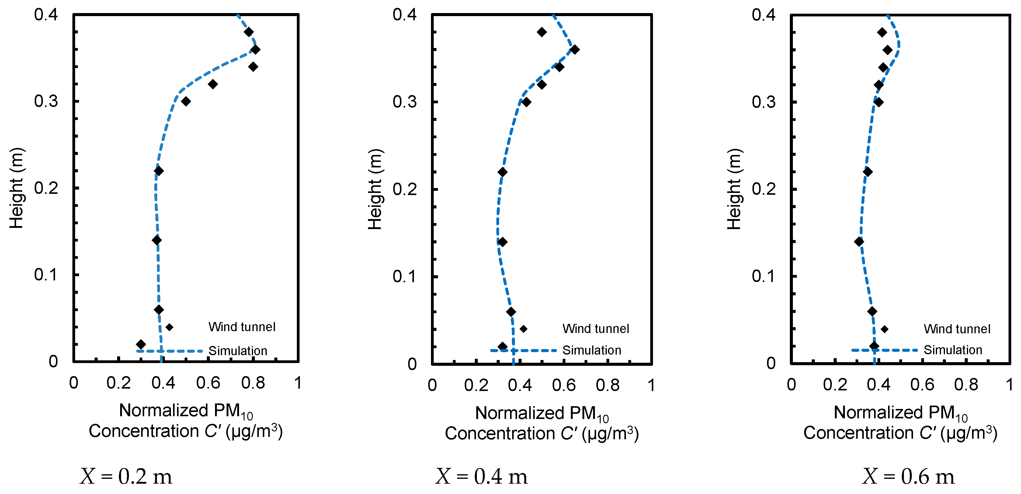
2.2.2. Particle Transportation in a Ventilated Chamber

Chen et al. analyzed the dispersion of particulate matter with a diameter of 10 μm inside a well-ventilated chamber [77]. Figure 4a represents the geometry of the chamber, where the air inlet and outlet (0.04 m × 0.04 m) are aligned with the middle plane (y = 0.2 m). In trials, particles were uniformly mixed with supplied air using a separator, and then injected into the chamber with a speed of 0.45 m/s. The model was built in the aforementioned way to calculate the normalized PM₁₀ concentration along three lines (x = 0.2, 0.4, and 0.6 m) of the central plane and compared with results of an identical chamber of PDA experiments (Figure 4a,c). Mean errors were 8.9, 7.2, and 5.3% on three lines of the central plane, respectively (Figure 5). To determine computational accuracy and cost, the model was parameterized to accurately forecast particle concentration making it feasible to simulate atmospheric particle transportation for the single-sided ventilation using the revised generalized drift flux model.

2.3. Simulation Setup

We built corresponding building and tree models to analyze the impact of outdoor trees on indoor particulate matter dispersion under natural ventilation. The procedures were quantitatively evaluated by simulating a series of test scenarios using different parameters: tree quantity (CVCs = 0.2, 0.8, 1.8, 3.2, and 5.0 m³/m²), window opening size (wall porosities = 3.5 and 7.0%), and oncoming wind velocity (u₀ = 1.0, 2.0, 3.0, and 4.0 m/s) (Figure 6).

The building was a typical auditorium surrounded by green space with an area of 8750 m² in total. The green space was divided into 14 equal units (25 m × 25 m), where trees were planted. The crown volume coverage (CVC) was introduced to represent trees planted in the green space and defined as crown volume per area of green space and expressed as [78]:

$$CVC{(\mathrm{m}}^3{/\mathrm{m}}^2)=\frac{{\mathrm{Total}\mathrm{crown}\mathrm{volume}\mathrm{in}\mathrm{green}\mathrm{space}(\mathrm{m}}^3)}{{\mathrm{Area}\mathrm{of}\mathrm{green}\mathrm{space}(\mathrm{m}}^2)}$$

(26)

For the simulated auditorium, there were 22 windows (4.8 m × 1.2 m for fully opened windows) on walls and 2 safety exits (2.4 m × 2.4 m) on both sides. The main entrance, front door is 7.6 m × 2.4 m. Cypress (Platycladus orientalis), a type of evergreen conifer, was selected in the model. The leaf area density, tree height, crown diameter and crown base height are 2.2 m²/m³, 5.0 m, 5.0 m and 2.0 m, respectively. The deposition velocities of cypress for PM_1.0, PM_2.5 and PM₁₀ are set to 0.1949, 0.0371 and 0.0615 m/s, respectively [13,71]. According to the literature [37,40], the leaf area index and height of grass are 2.0 m³/m³ and 0.5 m, respectively. Additionally, the deposition velocities of grass for PM_1.0, PM_2.5 and PM₁₀ are 0.02, 0.0028 and 0.0064 m/s, respectively.

The computational domain, with a dimension of 385 m × 255 m × 143 m, was divided into three types of structural hexahedral meshes (coarse meshes: X_min = Y_min = Z_min = 0.10H; fine meshes: X_min = Y_min = Z_min = 0.04H; and finest meshes: X_min = Y_min = Z_min = 0.02H) (Figure 7). After grid independence testing, fine mesh (X_min = Y_min = Z_min = 0.04H) with a total of 3.1 million cells was selected to ensure a higher resolution in the target region. The boundary setting was similar to that described in Section 2.2.1. The pollution sources were assumed to be transported pollutants diluted through the inlet boundary with no other pollution sources in the domain. In addition, infiltration of building walls was not accounted for in the model because natural ventilation flow rates at window openings were far stronger than those from infiltration. Other boundary conditions settings are shown in

Table 1. Boundary conditions setting *.

Parameter	Definition	Values
Location	Xi’an (China)	latitude: 34.26° N, longitude: 108.07° E
Meteorological conditions	wind speed at the height of 10 m	1.0, 2.0, 3.0, 4.0 m/s
	wind direction	North
Pollution source	PM1.0	85 μg/m3
	PM2.5	123 μg/m3
	PM10	225 μg/m3

* Since the highest air pollution level stretches from mid-November to December, average atmospheric particle concentrations and wind conditions (wind velocities and predominate wind direction) during this time period from the Xi’an statistical yearbook (2017) were selected as boundary parameters [79,80].

.

To further analyze relationships between natural ventilation potential and indoor particle concentrations, the natural ventilation rate was selected as an evaluation index. According to previous research [81,82], wind pressure is the main driving force of natural ventilation in the study area. Airflow penetrates buildings and trees as a consequence of pressure differences generated on building facades. Affected by wind deflection, the windward wind pressure of a building facade is generally positive, whereas the leeward is negative. Thus, the wind pressure on the facade of the building is expressed as:

P_w = 0.5C_pρV²

(27)

where P_w is wind pressure (Pa), C_p is a static pressure coefficient, ρ is air density (kg/m³), and V is wind velocity (m/s).

The natural ventilation rate is expressed as follows:

$$G=F_j\sqrt{\frac{2\left|\Delta P\right|\cdot \rho }{\left[{\left(\frac{F_j}{F_p}\right)}^2\frac{{\zeta }_p}{{\zeta }_j}+1\right]\cdot {\zeta }_j}}$$

(28)

where G is the natural ventilation rate (kg/s); F_j and F_p are the inlet and outlet area (m²), respectively; ζ_j and ζ_p are coefficients of local resistance at the inlet and outlet, set as 2.59 and 8, respectively [83]. |∆P| is the difference in wind pressure on the facade of windward and leeward sides of the buildings (Pa), and ρ is air density (kg/m³).

3. Results and Discussion

3.1. Baseline Scenario

Figure 8 depicts the contours of airflow fields and PM₁₀ distributions in the baseline scenario (oncoming wind velocity = 2.0 m/s, CVC = 0.8 m³/m², wall porosity = 3.5%). This demonstrated that the wind velocity increases dramatically at the turn of the windward wall. Airflows penetrate inwards from the north of the auditorium. The wind velocity slows gradually and reaches a minimum near the windward wall. An intense vortex forms in the west of the auditorium, where the wind velocity is relatively low. There are four small vortices and a relatively large vortex at the south of the auditorium. Inside the auditorium, airflows penetrate through areas where windows are open. This forms long and narrow ventilation corridors where wind velocity is relatively high. At the east of these ventilation corridors, the wind velocity is variable. A large vortex forms in the west of the auditorium, where the wind velocity is the lowest and uniform (Figure 8a). The windward wind velocity increases progressively with height and rises dramatically when airflows approach the roof (Figure 8c). Similar airflow patterns can be seen in an isolated room with perpendicular wind direction [84]. The windward airflow is separated at the front corner of the building, spreads around the top surface of the building and extends downwind. The wind velocity drops gradually with height and a small clockwise vortex forms near and above the windward wall in the indoor perpendicular direction. Airflows converge near the open windows on the leeward façade where the wind velocity is relatively high. Additionally, a counterclockwise vortex is formed in the turbulent wake area due to the aerodynamic and obstacle effects of trees on airflows.

Trees are effective in reducing atmospheric particles. PM₁₀ on both sides of the auditorium is higher than indoors with lanceolate distributions (Figure 8b). The indoor concentration is higher in wind corridors, ranging from 70 to 190 μg/m³. Re-circulation inside the auditorium creates a well-mixed zone with little variation in particle concentration. PM₁₀ is lower on windward tree canopies owing to the dust-retention ability of trees (Figure 8d). Due to gravitational deposition effects, the indoor particle concentration on the top of the space is lower than that near the ground, which is in accordance with the results of Jin et al. [84].

Particle concentrations differ in windward areas, where the longer the distance, the lower the concentrations (Figure 9). A relatively small concentration peak appears near the windward wall of the auditorium. Because airflows converge by windows, where the particles are blocked by walls, there is a slight increase in particle concentrations. Particle concentrations inside the auditorium decrease further from the windward side. In addition, the indoor concentration is 44 to 60% of that at the inlet values due to dust retention effects of plants and windows hindering particle diffusion towards the building interior. Due to turbulent diffusion, PM₁₀ declines most significantly, and the deposition rate is relatively high. However, at leeward sites, concentrations are all below 50 μg/m³ with smaller differences, regardless of particle size. Concentrations decline faster due to the deposition effect of trees around the leeward sites.

3.2. Oncoming Wind Speed and Window Opening Size

Oncoming wind velocities are set to 1.0, 2.0, 3.0, and 4.0 m/s to explore the effects of oncoming wind velocity on indoor particle concentration distributions (Figure 10). For clarity, only scenarios where CVC = 0.8 m³/m² are presented. Particle concentrations tend to increase exponentially with the increasing oncoming wind velocity whether windows are half or fully open. This appears to because the increased wind velocity enhances indoor/outdoor cross ventilation and particle diffusion. This result is contrary to research indicating a negative correlation between normalized oncoming wind speed and average indoor particle concentrations [61]. The reason is that polluted sources in their study originated from traffic, while our study assumed that the pollution sources were wind transported and diluted through the inlet. Among wind velocity increments, average indoor concentrations differ more significantly among PM_1.0, PM_2.5 and PM₁₀.These differences are slight in PM₁₀, PM_2.5 and PM_1.0 when wind velocity is 1.0 m/s. However, PM₁₀ and PM_2.5 differ by 35 μg/m³ when the wind velocity reaches 4.0 m/s. PM₁₀ varies most significantly with wind velocity, followed by PM_2.5 and PM_1.0 successively, as increasing wind velocity facilitates turbulent diffusion of larger particles and diminishes surface deposition.

This section focuses on the effect of window opening size on indoor particle concentrations. For clarity, indoor and outdoor PM₁₀ is compared when windows are fully open (wall porosity = 7.0%) and half open (wall porosity = 3.5%) in the baseline scenario (Figure 11). PM₁₀ is similar on the windward facade of the auditorium when windows are half or fully open. The airflow converges in relatively small areas and the wind velocity increases when the wall porosity is 3.5%, the turbulent diffusion accelerates as a result. Hence, the indoor PM₁₀ is higher than that when the wall porosity is 7.0%. This result agrees well with the study demonstrating that 9% wall porosity resulted in greater normalized concentrations compared with 18% [61]. The difference reaches its maximum when windows are half and fully open within 70 m ≤ X ≤ 75 m, at approximately 30 μg/m³. This means an increment of 20% in PM₁₀ results by closing the windows by half. Near leeward windows, the concentration drops faster when the wall porosity is 3.5%. At leeward sites, the difference decreases gradually and the concentration is approximately the same when 0 m < X < 12.5 m, whether the wall porosity is 3.5% or 7.0%.

3.3. Crown Volume Coverage

Particle concentrations decline gradually with increasing CVC, and PM₁₀ varies within the widest range (Figure 12). At windward sites, concentrations decline gradually as the distance to the inlet boundary increases. This decrease is most striking when CVCs equal 3.2 and 5.0 m³/m². Concentrations increase and reach a peak at about 10 m from windward windows. The higher the CVC, the more evident the peak. Wind velocity and airflow are lower when CVC is higher. Thus, natural ventilation is affected, and cross ventilation becomes weaker, resulting in an increase in particle concentration. Inside the auditorium, the difference of PM₁₀ approaches 50 μg/m³ when CVCs are 0.2 and 5.0 m³/m² (Figure 12a). The difference of PM_1.0 changes consistently with distance. When CVCs are 1.8, 3.2 and 5.0 m³/m², the concentration difference is relatively small along the horizontal plane (Figure 12c). At leeward sites, particle concentrations decline initially and then increase gradually as the distance from the auditorium increases, and concentration changes tend to be consistent irrespective of CVC.

Average particle concentrations at pedestrian level (1.5 m height) in windward, indoor and leeward sites among various CVCs with oncoming wind velocity of 2.0 m/s and wall porosity of 3.5% scenarios are shown in Figure 13. Concentration distributions clearly differ between windward and leeward sites. Trees planted in windward and leeward sites intercepted particles and reduced the kinetic energy of airflow resulting from the shelter effect of tree canopies. Hence, particulate dispersion was impeded by trees in windward and leeward sites. The concentrations decrease with the increase of CVCs. At windward sites, concentrations clearly decline with increasing CVCs. The indoor and leeward sites have the smallest particle concentrations when CVC is 1.8 m³/m². It is also evident that PM₁₀ differences among various CVCs are larger than those of PM_1.0 and PM_2.5. Moreover, with CVC increasing, the declining tendency of concentrations became lower when CVCs > 1.8 m³/m².

Tree planting density imposes relatively significant impacts on particle concentration distributions [85]. These observations show that the oncoming wind velocity is positively correlated with indoor particle concentration, prompting us to examine connections between CVC and indoor concentration in scenarios when the oncoming wind velocity is 4.0 m/s and wall porosity is 3.5% (Figure 14). Particle concentration and CVC exhibit significant quadratic patterns. Concentrations decline gradually with CVC initially and then increase slowly. This tendency is similar to the results of Yin et al. [78]. PM₁₀, PM_2.5 and PM_1.0 reach their minima (52.4 μg/m³ for PM₁₀, 34.5 μg/m³ for PM_2.5, and 16.5 μg/m³ for PM_1.0) when CVCs are 4.12, 4.73, and 3.59 m³/m², respectively. Average indoor PM₁₀ concentration fluctuates most significantly with CVC, while PM_2.5 and PM_1.0 change slowly, because larger sized particles are more readily deposited on leaves [86].

The World Health Organization air quality guidelines (WHO AQGs) identify PM_2.5 as an indicator for particulate matter evaluation. We selected interim target-3 (IT-3) with a PM_2.5 of 37.5 μg/m³ as a criterion [87]. When CVC > 2.87 m³/m², PM_2.5 concentration is below 37.5 μg/m³ and achieves the IT-3 of WHO AQG for 24-hour mean concentrations. Above all, the indoor PM_2.5 is in line with WHO AQG specifications when 2.87 m³/m² ≤ CVC ≤ 4.73 m³/m².

3.4. Relationship Between Indoor Particle Concentrations and Natural Ventilation Rate (G)

The relationship between indoor average particle concentration and natural ventilation rate (G) varied among the simulations (Figure 15). Average indoor concentration and natural ventilation rate show a similar trend and a positive correlation. PM₁₀ changes most significantly with the natural ventilation rate. Indoor particle concentration clearly increases when the wall porosity is 3.5% compared with that when the wall porosity is 7.0%, because the natural ventilation rate is higher when windows are fully open. When the air exchange frequency is constant, airflow discharges rapidly, removing pollutants and reducing indoor particulate matter. Previous studies have demonstrated that absolute or relative difference in wind pressure in buildings is weakly correlated with indoor particle concentrations [58,88]. Our simulation results indicate that the natural ventilation rate is significantly and positively correlated with indoor particle concentration linked to window opening size. Previous research has also shown that indoor and outdoor particulate concentrations are closely correlated (R² = 0.9104) when windows are closed and there are no obvious indoor pollution sources. The indoor/outdoor concentrations ratios (I/O ratios) were significantly correlated with outdoor wind velocity and relative humidity [56]. Our results were based on having the windows open (half open), thus expanding the understanding of relationships on indoor/outdoor particulate matter transportation.

In this study, the impact of outdoor trees on PM_1.0, PM_2.5 and PM₁₀ inside a typical auditorium was analyzed using numerical simulations. Like the I/O ratio, this CFD method may be used as an alternative approach to investigate relationships between indoor and outdoor particle concentration distributions, especially when trees are planted outside. For future consideration, our study points to some simulation improvements. First, green spaces, by definition, have trees, shrubs and/or herbs. Our study only modeled the impact of trees and herbs, leaving open the question of more diverse green space configurations. Further, this study used CVC to quantify the trees outside, which does not reflect the distribution pattern or arrangement of trees. This may exert a different influence on the indoor particulate matter dispersion. Future simulations should take into account the coupling effects of tree distribution patterns on microclimate. Second, airflow is variable and affects particulate diffusion even it is constant, but our simulations set the particles as a steady state without affecting airflow. Hence, our conclusions remain to be validated by more field experiments. Third, the impact of plants on dust retention changes with growth, suggesting that dynamic vegetation growth should be included in future simulations. Fourth, previous research has shown that temperature and solar radiation were weakly correlated with indoor particulate matter (R² = 0.32–0.47 for temperature and R² = 0.06–0.15 for solar radiation) [55]. However, the effects of solar radiation, and heat transfer between buildings and plants were not taken into account in this simulation. Nevertheless, these factors should be considered in future studies, so that simulation results can better reflect actual conditions. Finally, we did not consider indoor generated particle sources in our simulations. We exclude them because our focus was on the effect of outdoor trees on indoor particle concentration distributions, but in the real built environment, indoor air pollution is affected not only by outdoor pollutants, but also indoor-generated sources, i.e., cooking, smoking, cleaning, and general activity. A comprehensive analysis concerning outdoor/indoor polluted sources, particle penetration and infiltration should be conducted to thoroughly understand outdoor and indoor particle transportation in built environments.

4. Conclusions

We adapted computational fluid dynamics (CFD) models, considering the aerodynamic and deposition effect of trees, to investigate the impact of outdoor trees on indoor PM_1.0, PM_2.5 and PM₁₀ concentration distributions. Using CVC as an evaluation index for outdoor tree planting, our study thoroughly compared indoor particle concentration distributions with different CVCs, oncoming wind velocities, window opening sizes, and the capacity of natural ventilation potential. The following conclusions can be drawn:

(1)

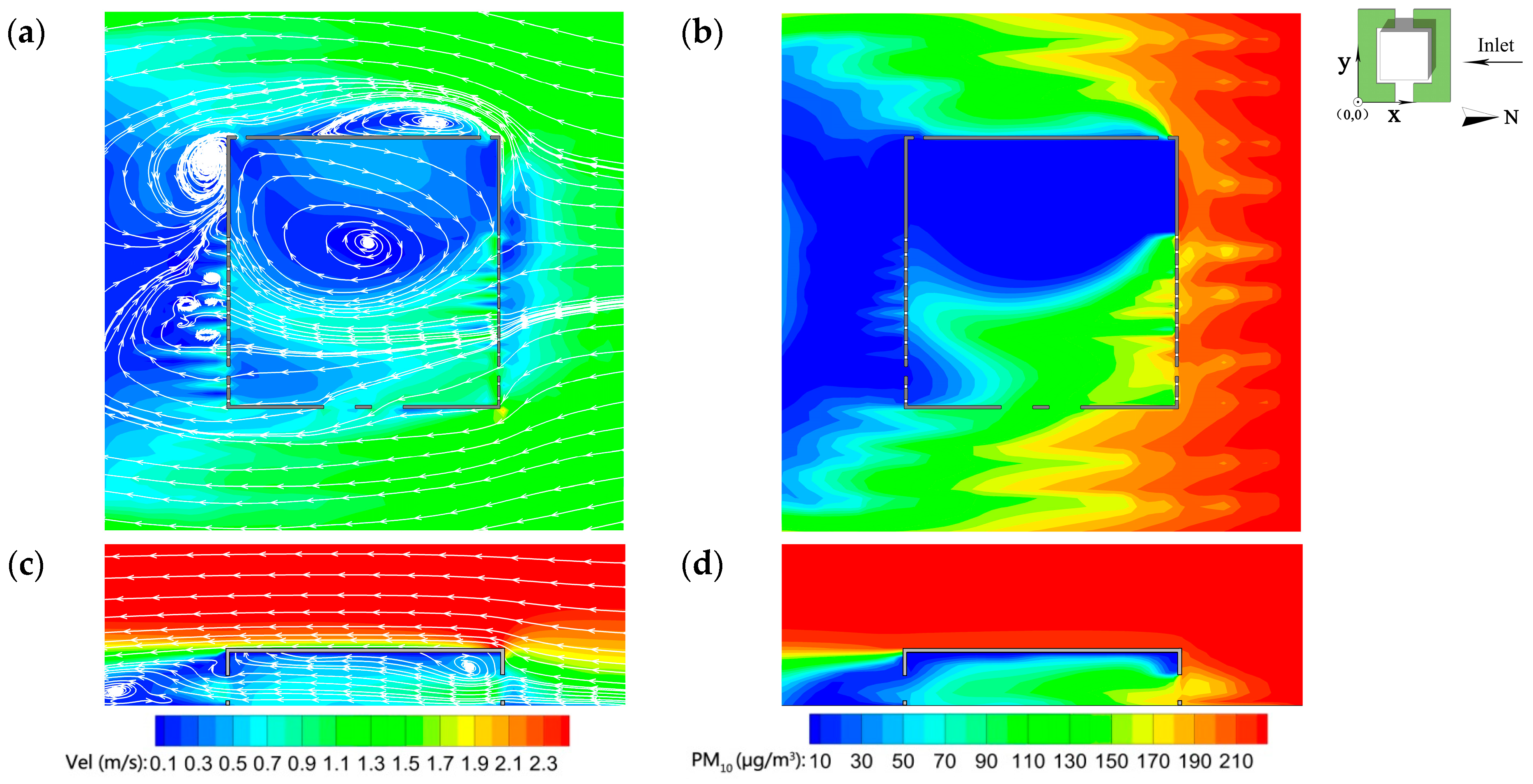
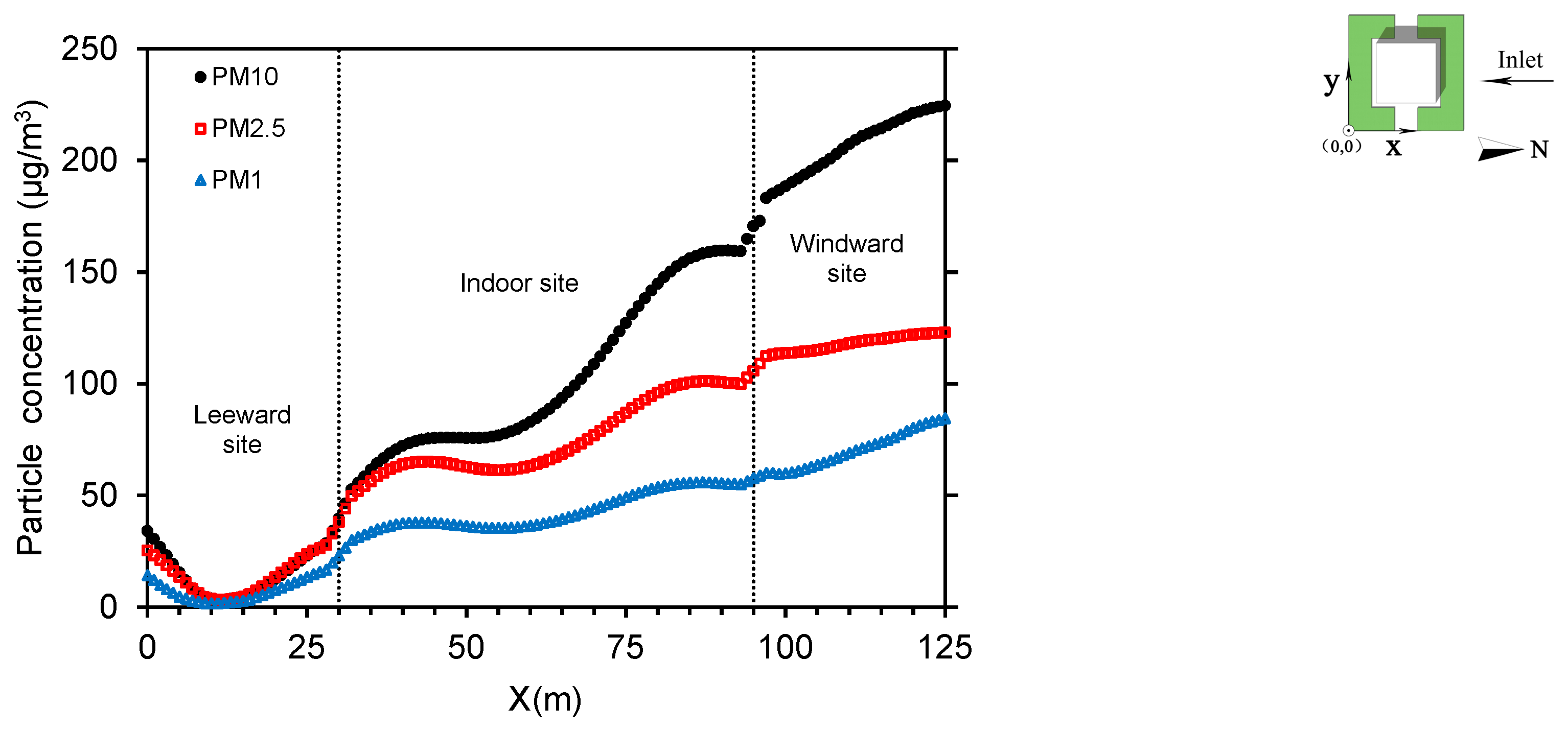
The building envelope restricts airflow and particle dispersion and dilution. In our baseline scenario, a relatively large vortex formed inside the auditorium. As a consequence, the inside air re-circulated and created a well-mixed zone with little variation in particle concentration. Inside the auditorium, the concentration declined with increased distance from the windward side. In addition, the concentration inside was 44 to 60% of that at the inlet boundary, because the dust-retaining ability of trees and window area obstructed diffusion of particles to indoors. Indoor PM₁₀ fluctuated most significantly with increasing distance from the inlet boundary. PM_2.5 and PM_1.0 changes were not clear because the deposition was more effective among larger particles due to turbulent diffusion.

(2)

Under the assumption that pollution sources were diluted through the inlet, the average indoor particle concentration rose exponentially with increasing oncoming wind speed. The difference among PM_1.0, PM_2.5 and PM₁₀ was relatively small when wind velocity was 1.0 m/s, but the concentration changed significantly as the wind velocity increased to 2.0 m/s. As increased wind velocity intensified turbulent diffusion of larger particles and reduced surface deposition, PM₁₀ changed most significantly, followed by PM_2.5 and PM_1.0.

(3)

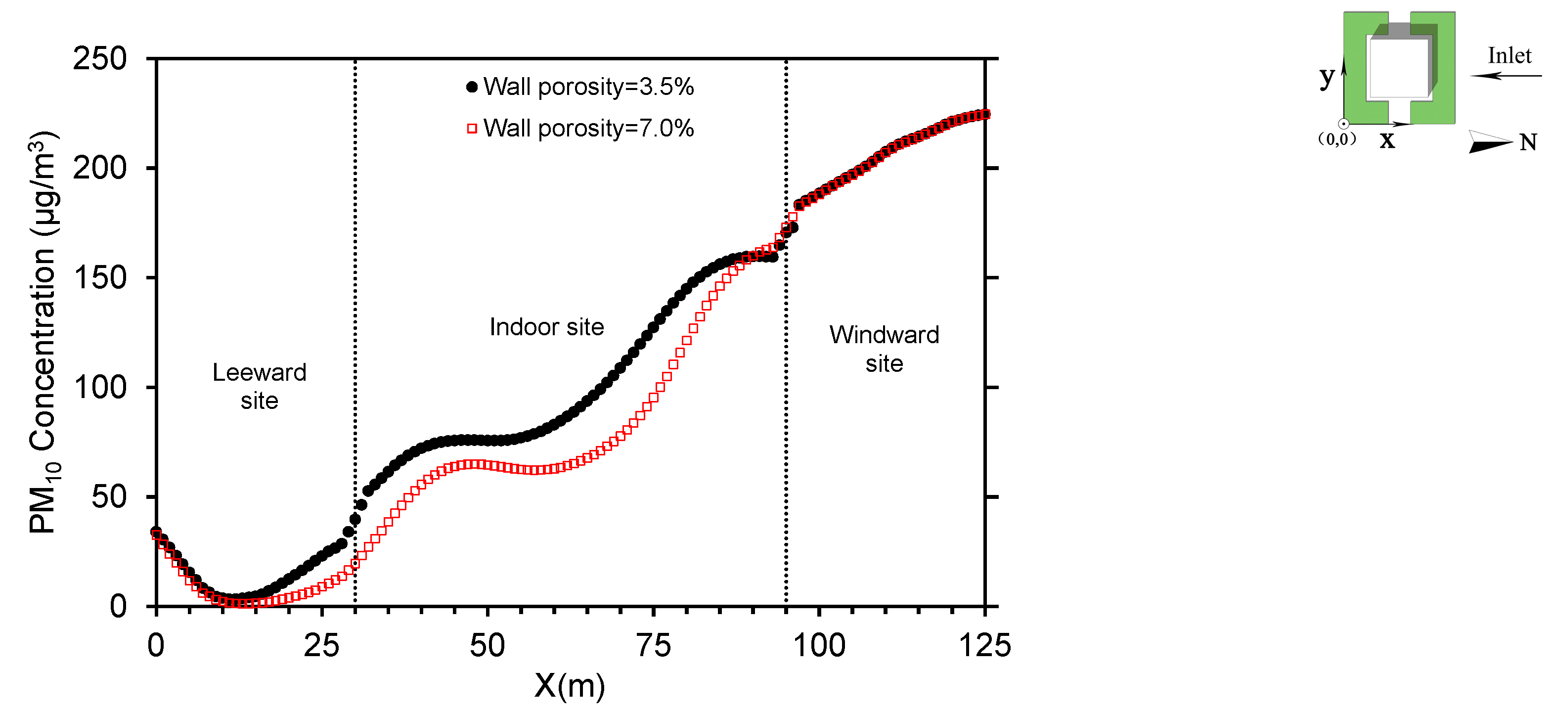
Indoor cross-ventilation was improved when the wall porosity was 7.0%. Thus a 20% increment in PM₁₀ was achieved by closing windows by half. Near the leeward windows, the concentration declined much more quickly when the wall porosity was 3.5% than that when the wall porosity was 7.0%. The difference gradually narrowed as the distance to the leeward wall increased and the concentration was very similar under the condition when 0 m < X < 12.5 m.

(4)

The average indoor particle concentration declined initially and then increased with a higher CVC. When the CVC ranged between 2.87 and 4.73 m²/m³, the indoor PM_2.5 concentration could meet the requirement of IT-3 of the WHO AQGs for 24-hour mean concentrations.

(5)

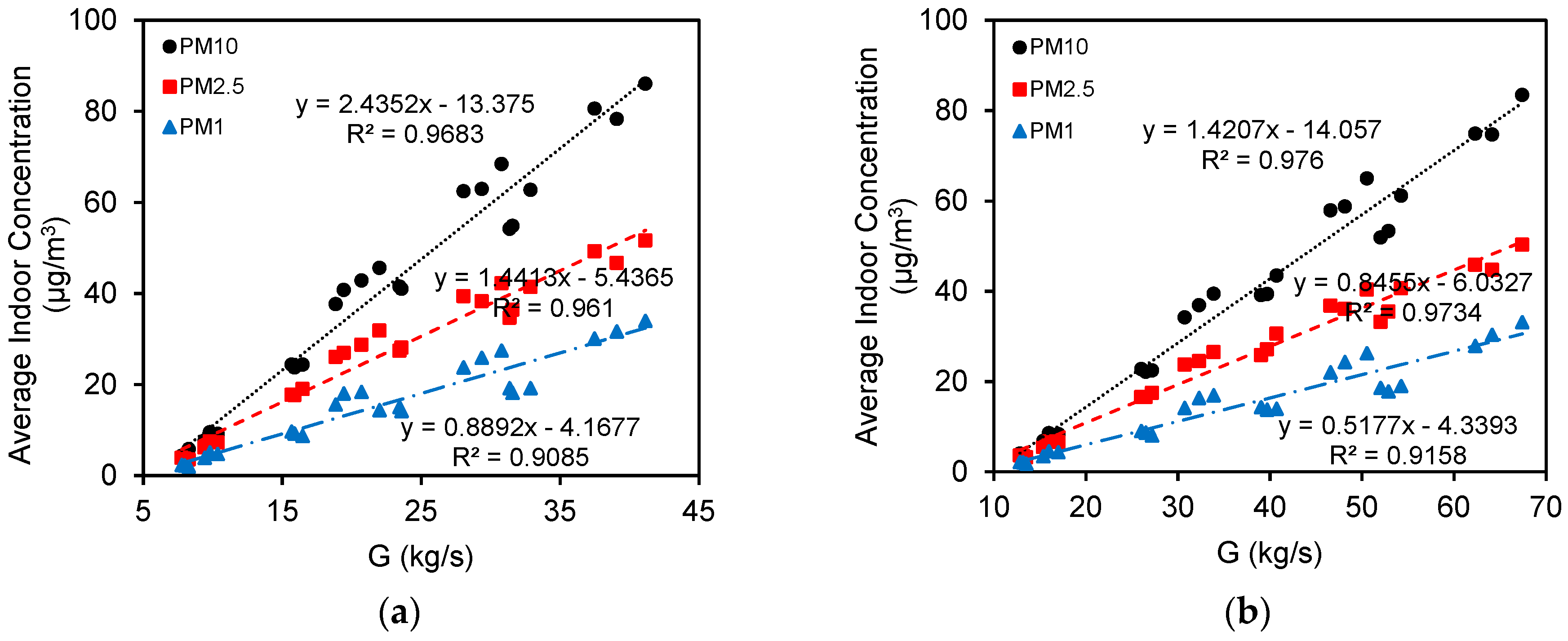
Average indoor concentrations were positively correlated with natural ventilation rates and increased more quickly when the wall porosity was 3.5%. Airflow removed more pollutants and shortened longevity of particles indoors when the wall porosity was 7.0%. Thus, the indoor particle concentration was lower than that when the wall porosity was 3.5%.

Our findings indicate that trees planted around buildings, window opening size, and predominate wind velocity all have significant impacts on indoor atmospheric particle concentrations. To plan new buildings, it will be necessary to deliberately evaluate tree planting designs and ambient wind conditions around buildings at early design stages. Such planning will maximize the natural ventilation potential while decreasing the indoor particle concentration. Further, ventilation strategies (changing window opening size), outdoor movable tree planting pools, and layout of interior space may be adapted for existing buildings, so as to lower the indoor particle concentrations. Our conclusions could be used as guidelines for assisting building architects, urban planners and landscape architects to evaluate natural ventilation strategies with enhanced consideration for improving indoor air quality in public buildings.

References

1. Tong, Z.; Yang, B.; Hopke, P.K.; Zhang, K.M. Microenvironmental air quality impact of a commercial-scale biomass heating system. Environ. Pollut. 2017, 220, 1112–1120. [Google Scholar] [CrossRef] [PubMed]
2. Dou, H.; Ming, T.; Li, Z.; Peng, C.; Zhang, C.; Fu, X. Numerical simulation of pollutant dispersion characteristics in a three-dimensional urban traffic system. Atmos. Pollut. Res. 2018, 9, 735–746. [Google Scholar] [CrossRef]
3. Brunekreef, B.; Holgate, S.T. Air pollution and health. Lancet 2002, 360, 1233–1242. [Google Scholar] [CrossRef]
4. Karottki, D.G.; Spilak, M.; Frederiksen, M.; Andersen, Z.J.; Madsen, A.M.; Ketzel, M.; Massling, A.; Gunnarsen, L.; Møller, P.; Loft, S. Indoor and outdoor exposure to ultrafine, fine and microbiologically derived particulate matter related to cardiovascular and respiratory effects in a panel of elderly urban citizens. Int. J. Environ. Res. Public Health 2015, 12, 1667–1686. [Google Scholar] [CrossRef]
5. Magalhaes, S.; Baumgartner, J.; Weichenthal, S. Impacts of exposure to black carbon, elemental carbon, and ultrafine particles from indoor and outdoor sources on blood pressure in adults: A review of epidemiological evidence. Environ. Res. 2018, 161, 345–353. [Google Scholar] [CrossRef] [PubMed]
6. Nowak, D.J.; Hirabayashi, S.; Doyle, M.; McGovern, M.; Pasher, J. Air pollution removal by urban forests in Canada and its effect on air quality and human health. Urban For. Urban Green. 2018, 29, 40–48. [Google Scholar] [CrossRef]
7. Chen, C.; Zhao, B. Review of relationship between indoor and outdoor particles: I/O ratio, infiltration factor and penetration factor. Atmos. Environ. 2011, 45, 275–288. [Google Scholar] [CrossRef]
8. Zhang, S.; Wu, Y.; Liu, H.; Huang, R.; Yang, L.; Li, Z.; Fu, L.; Hao, J. Real-world fuel consumption and CO2 emissions of urban public buses in Beijing. Appl. Energy 2014, 113, 1645–1655. [Google Scholar] [CrossRef]
9. Janhäll, S. Review on urban vegetation and particle air pollution-Deposition and dispersion. Atmos. Environ. 2015, 105, 130–137. [Google Scholar] [CrossRef]
10. Gallagher, J.; Baldauf, R.; Fuller, C.H.; Kumar, P.; Gill, L.W.; McNabola, A. Passive methods for improving air quality in the built environment: A review of porous and solid barriers. Atmos. Environ. 2015, 120, 61–70. [Google Scholar] [CrossRef]
11. Ould-Dada, Z.; Baghini, N.M. Resuspension of small particles from tree surfaces. Atmos. Environ. 2001, 35, 3799–3809. [Google Scholar] [CrossRef]
12. Ould-Dada, Z. Dry deposition profile of small particles within a model spruce canopy. Sci. Total Environ. 2002, 286, 83–96. [Google Scholar] [CrossRef]
13. Freer-Smith, P.H.; Beckett, K.P.; Taylor, G. Deposition velocities to Sorbus aria, Acer campestre, Populus deltoides× trichocarpa ‘Beaupré’,Pinus nigra and× Cupressocyparis leylandii for coarse, fine and ultra-fine particles in the urban environment. Environ. Pollut. 2005, 133, 157–167. [Google Scholar] [CrossRef] [PubMed]
14. Mori, J.; Hanslin, H.M.; Burchi, G.; Sæbø, A. Particulate matter and element accumulation on coniferous trees at different distances from a highway. Urban For. Urban Green. 2015, 14, 170–177. [Google Scholar] [CrossRef]
15. Xie, C.; Kan, L.; Guo, J.; Jin, S.; Li, Z.; Chen, D.; Li, X.; Che, S. A dynamic processes study of PM retention by trees under different wind conditions. Environ. Pollut. 2018, 233, 315–322. [Google Scholar] [CrossRef] [PubMed]
16. Baidurela, A.; Halik, Ü.; Aishan, T.; Nuermaimaiti, K. Maximum dust retention of main greening trees in arid land oasis cities, Northwest China. Sci. Silvae Sin. 2015, 51, 57–63. [Google Scholar]
17. Fan, S.Y.; Yan, H.; Qishi, M.Y.; Bai, W.L.; Pi, D.J.; Li, X.; Dong, L. Dust capturing capacities of twenty-six deciduous broad-leaved trees in Beijing. J. Plant Ecol. 2015, 39, 736–745. [Google Scholar]
18. Dzierżanowski, K.; Gawroński, S.W. Use of trees for reducing particulate matter pollution in air. Chall. Mod. Technol. 2011, 2, 69–73. [Google Scholar]
19. Przybysz, A.; Sæbø, A.; Hanslin, H.M.; Gawroński, S.W. Accumulation of particulate matter and trace elements on vegetation as affected by pollution level, rainfall and the passage of time. Sci. Total Environ. 2014, 481, 360–369. [Google Scholar] [CrossRef]
20. Sgrigna, G.; Sæbø, A.; Gawronski, S.W.; Popek, R.; Calfapietra, C. Particulate matter deposition on Quercus ilex leaves in an industrial city of central Italy. Environ. Pollut. 2015, 197, 187–194. [Google Scholar] [CrossRef]
21. Chen, L.X.; Liu, C.M.; Zou, R.; Yang, M.; Zhang, Z.Q. Experimental examination of effectiveness of vegetation as bio-filter of particulate matter in the urban environment. Environ. Pollut. 2016, 208, 198–208. [Google Scholar] [CrossRef]
22. Zhang, Z.D.; Xi, B.Y.; Cao, Z.G.; Jia, L.M. Exploration of a quantitative methodology to characterize the retention of PM2.5 and other atmospheric particulate matter by plant leaves: Taking Populus tomentosa as an example. Chin. J. Appl. Ecol. 2014, 25, 2238–2242. [Google Scholar]
23. Song, Y.S.; Maher, B.A.; Li, F.; Wang, X.K.; Sun, X. Particulate matter deposited on leaf of five evergreen species in Beijing, China: Source identification and size distribution. Atmos. Environ. 2015, 105, 53–60. [Google Scholar] [CrossRef] [Green Version]
24. Yan, J.; Lin, L.; Zhou, W.; Ma, K.; Pickett, S.T.A. A novel approach for quantifying particulate matter distribution on leaf surface by combining SEM and object-based image analysis. Remote Sens. Environ. 2016, 173, 156–161. [Google Scholar] [CrossRef] [Green Version]
25. Leonard, R.J.; McArthur, C.; Hochuli, D.F. Particulate matter deposition on roadside plants and the importance of leaf trait combinations. Urban For. Urban Green. 2016, 20, 249–253. [Google Scholar] [CrossRef]
26. Liu, J.; Cao, Z.; Zou, S.; Liu, H.; Hai, X.; Wang, S.; Duan, J.; Xi, B.; Yan, G.; Zhang, S.; et al. An investigation of the leaf retention capacity, efficiency and mechanism for atmospheric particulate matter of five greening tree species in Beijing, China. Sci. Total Environ. 2018, 616–617, 417–426. [Google Scholar] [CrossRef] [PubMed]
27. Xu, Y.; Xu, W.; Mo, L.; Heal, M.R.; Xu, X.; Yu, X. Quantifying particulate matter accumulated on leaves by 17 species of urban trees in Beijing, China. Environ. Sci. Pollut. Res. 2018, 25, 12545–12556. [Google Scholar] [CrossRef] [PubMed]
28. Hagler, G.S.W.; Lin, M.Y.; Khlystov, A.; Baldauf, R.W.; Isakov, V.; Faircloth, J.; Jackson, L.E. Field investigation of roadside vegetative and structural barrier impact on near-road ultrafine particle concentrations under a variety of wind conditions. Sci. Total Environ. 2012, 419, 7–15. [Google Scholar] [CrossRef] [PubMed]
29. Tong, Z.; Whitlow, T.H.; MacRae, P.F.; Landers, A.J.; Harada, Y. Quantifying the effect of vegetation on near-road air quality using brief campaigns. Environ. Pollut. 2015, 201, 141–149. [Google Scholar] [CrossRef]
30. Lu, S.; Yang, X.; Li, S.; Chen, B.; Jiang, Y.; Wang, D.; Xu, L. Effects of plant leaf surface and different pollution levels on PM2.5 adsorption capacity. Urban For. Urban Green. 2018, 34, 64–70. [Google Scholar] [CrossRef]
31. Sæbø, A.; Popek, R.; Nawrot, B.; Hanslin, H.M.; Gawronska, H.; Gawronski, S.W. Plant species differences in particulate matter accumulation on leaf surfaces. Sci. Total Environ. 2012, 427–428, 347–354. [Google Scholar] [CrossRef] [PubMed]
32. Liu, L.; Guan, D.; Peart, M.R.; Wang, G.; Zhang, H.; Li, Z. The dust retention capacities of urban vegetation-a case study of Guangzhou, South China. Environ. Sci. Pollut. Res. 2013, 20, 6601–6610. [Google Scholar] [CrossRef] [PubMed]
33. Liu, J.; Zhu, L.; Wang, H.; Yang, Y.; Liu, J.; Qiu, D.; Ma, W.; Zhang, Z.; Liu, J. Dry deposition of particulate matter at an urban forest, wetland and lake surface in Beijing. Atmos. Environ. 2016, 125, 178–187. [Google Scholar] [CrossRef]
34. Giardina, M.; Buffa, P. A new approach for modeling dry deposition velocity of particles. Atmos. Environ. 2018, 180, 11–22. [Google Scholar] [CrossRef]
35. Buccolieri, R.; Gromke, C.; Sabatino, S.D.; Ruck, B. Aerodynamic effects of trees on pollutant concentrationin street canyons. Sci. Total Environ. 2009, 407, 5247–5256. [Google Scholar] [CrossRef] [PubMed]
36. Buccolieri, R.; Salim, S.M.; Leo, L.S.; Sabatino, S.D.; Chan, A.; Ielpo, P.; Gennaro, G.; Gromke, C. Analysis oflocal scale tree-atmosphere interaction on pollutant concentration in idealized street canyons and applicationto a real urban junction. Atmos. Environ. 2011, 45, 1702–1713. [Google Scholar] [CrossRef]
37. Pugh, T.A.; Mackenzie, A.R.; Whyatt, J.D.; Hewitt, C.N. Effectiveness of green infrastructure for improvement of air quality in urban street canyons. Environ. Sci. Technol. 2012, 46, 7692–7699. [Google Scholar] [CrossRef] [PubMed]
38. Wania, A.; Bruse, M.; Blond, N.; Weber, C. Analysing the influence of different street vegetation ontraffic-induced particle dispersion using microscale simulations. J. Environ. Manag. 2012, 94, 91–101. [Google Scholar] [CrossRef]
39. Gromke, C.; Blocken, B. Influence of avenue-trees on air quality at the urban neighborhood scale. Part I: Quality assurance studies and turbulent Schmidt number analysis for RANS CFD simulations. Environ. Pollut. 2015, 196, 214–223. [Google Scholar] [CrossRef] [PubMed] [Green Version]
40. Jeanjean, A.P.R.; Monks, P.S.; Leigh, R.J. Modelling the effectiveness of urban trees and grass on PM2.5reduction via dispersion and deposition at a city scale. Atmos. Environ. 2016, 147, 1–10. [Google Scholar] [CrossRef]
41. Hofman, J.; Bartholomeus, H.; Janssen, S.; Calders, K.; Wuyts, K.; Van Wittenberghe, S.; Samson, R. Influence of tree crown characteristics on the local PM10 distribution inside an urban street canyon in Antwerp (Belgium): A model and experimental approach. Urban For. Urban Green. 2016, 20, 265–276. [Google Scholar] [CrossRef]
42. Tong, Z.; Baldauf, R.W.; Isakov, V.; Deshmukhd, P.; Zhang, K.M. Roadside vegetation barrier designs to mitigate near-road air pollution impacts. Sci. Total Environ. 2016, 541, 920–927. [Google Scholar] [CrossRef] [PubMed]
43. Hong, B.; Lin, B.; Qin, H. Numerical investigation on the coupled effects of building-tree arrangements on fine particulate matter (PM2.5) dispersion in housing blocks. Sustain. Cities Soc. 2017, 34, 358–370. [Google Scholar] [CrossRef]
44. Hong, B.; Qin, H.; Jiang, R. Are green walls better options than green roofs for mitigating PM10 pollution? CFD simulations in urban street canyons. Sustainability 2018, 10, 2833. [Google Scholar]
45. Buccolieri, R.; Santiago, J.; Rivas, E.; Sanchez, B. Review on urban tree modelling in CFD simulations: Aerodynamic, deposition and thermal effects. Urban For. Urban Green. 2018, 31, 212–220. [Google Scholar] [CrossRef]
46. Cardinale, N.; Micucci, M.; Ruggiero, F. Analysis of energy saving using natural ventilation in a traditional Italian building. Energy Build. 2003, 35, 153–159. [Google Scholar] [CrossRef]
47. Gratia, E.; De Herde, A. Natural cooling strategies efficiency in an office building with a double-skin façade. Energy Build. 2004, 36, 1139–1152. [Google Scholar] [CrossRef]
48. Yang, Z.; Shen, J.; Gao, Z. Ventilation and air quality in student dormitories in China: A case study during summer in Nanjing. Int. J. Environ. Res. Public Health 2018, 15, 132. [Google Scholar] [CrossRef]
49. Morawska, L.; Afshari, A.; Bae, G.N.; Buonanno, G.; Chao, C.Y.H.; Hänninen, O.; Hofmann, W.; Isaxon, C.; Jayaratne, E.R.; Pasanen, P.; et al. Indoor aerosols: From personal exposure to risk assessment. Indoor Air 2013, 23, 462–487. [Google Scholar] [CrossRef]
50. Tong, Z.; Chen, Y.; Malkawi, A.; Liu, Z.; Freeman, R.B. Energy saving potential of natural ventilation in China: The impact of ambient air pollution. Appl. Energy 2016, 179, 660–668. [Google Scholar] [CrossRef] [Green Version]
51. Yuan, Y.; Luo, Z.; Liu, J.; Wang, Y.; Lin, Y. Health and economic benefits of building ventilation interventions for reducing indoor PM2.5exposure from both indoor and outdoor origins in urban Beijing, China. Sci. Total Environ. 2018, 626, 546–554. [Google Scholar] [CrossRef] [PubMed]
52. Chatoutsidou, S.E.; Ondracek, J.; Tesar, O.; Tørseth, K.; Zdímal, V.; Lazaridis, M. Indoor/outdoor particulate matter number and mass concentration in modern offices. Build. Environ. 2015, 92, 462–474. [Google Scholar] [CrossRef] [Green Version]
53. Wang, F.; Meng, D.; Li, X.; Tan, J. Indoor-outdoor relationships of PM2.5 in four residential dwellings in winter in the Yangtze River Delta, China. Environ. Pollut. 2016, 215, 280–289. [Google Scholar] [CrossRef] [PubMed]
54. Jodeh, S.; Hasan, A.R.; Amarah, J.; Judeh, F.; Salghi, R.; Lgaz, H.; Jodeh, W. Indoor and outdoor air quality analysis for the city of Nablus in Palestine: Seasonal trends of PM10, PM5.0, PM2.5, and PM1.0 of residential homes. Air Qual. Atmos. Health 2018, 11, 229–237. [Google Scholar] [CrossRef]
55. Lee, B.H.; Yee, S.W.; Kang, D.H.; Yeo, M.S.; Kim, K.W. Multi-zone simulation of outdoor particle penetration and transport in a multi-story building. Build. Simul. 2017, 10, 525–534. [Google Scholar] [CrossRef]
56. Zhao, L.; Chen, C.; Wang, P.; Chen, Z.; Cao, S.; Wang, Q.; Xie, G.; Wan, Y.; Wang, Y.; Lu, B. Influence of atmospheric fine particulate matter (PM2.5) pollution on indoor environment during winter in Beijing. Build. Environ. 2015, 87, 283–291. [Google Scholar] [CrossRef]
57. Shao, Z.; Bi, J.; Ma, Z.; Wang, J. Seasonal trends of indoor fine particulate matter and its determinants in urban residences in Nanjing, China. Build. Environ. 2017, 125, 319–325. [Google Scholar] [CrossRef]
58. Chithra, V.S.; Shiva Nagendra, S.M. Impact of outdoor meteorology on indoor PM10, PM2.5 and PM1 concentrations in a naturally ventilated classroom. Urban Clim. 2014, 10, 77–91. [Google Scholar] [CrossRef]
59. Deng, G.; Li, Z.; Wang, Z.; Gao, J.; Xu, Z.; Li, J.; Wang, Z. Indoor/outdoor relationship of PM2.5concentration in typical buildings with and without air cleaning in Beijing. Indoor Built Environ. 2017, 26, 60–68. [Google Scholar] [CrossRef]
60. Amato, F.; Rivas, I.; Viana, M.; Moreno, T.; Bouso, L.; Reche, C.; Àlvarez-Pedrerol, M.; Alastuey, A.; Sunyer, J.; Querol, X. Sources of indoor and outdoor PM2.5 concentrations in primary schools. Sci. Total Environ. 2014, 490, 757–765. [Google Scholar] [CrossRef]
61. Tong, Z.; Chen, Y.; Malkaw, A.; Adamkiewicz, G.; Spengler, J.D. Quantifying the impact of traffic-related air pollution on the indoor air quality of a naturally ventilated building. Environ. Int. 2016, 89–90, 138–146. [Google Scholar] [CrossRef] [PubMed]
62. Franke, J.; Hellsten, A.; Schlunzen, K.H.; Carissimo, B. The COST 732 best practice guideline for CFD simulation of flows in the urban environment: A summary. Int. J. Environ. Pollut. 2011, 44, 419–427. [Google Scholar] [CrossRef]
63. Lin, B.; Li, X.; Zhu, Y.; Qin, Y. Numerical simulation studies of the different vegetation patterns’ effect on outdoor pedestrian thermal comfort. J. Wind Eng. Ind. Aerod. 2008, 96, 1707–1718. [Google Scholar] [CrossRef]
64. Amorim, J.H.; Rodrigues, V.; Tavares, R.; Valente, J.; Borrego, C. CFD modeling of the aerodynamic effect of trees on urban air pollution dispersion. Sci. Total Environ. 2013, 461, 541–551. [Google Scholar] [CrossRef] [PubMed]
65. Katul, G.; Mahrt, L.; Poggi, D.; Sanz, C. One-and two-equation models for canopy turbulence. Bound. Layer Meteorol. 2004, 113, 81–109. [Google Scholar] [CrossRef]
66. Kimura, A. Optimization of plant canopy model for reproducing aerodynamic effects of trees: Comparison between the canopy model optimized by the present authors and that proposed by Green. In Proceedings of Transactions of Architecture Institute of Japan; Architectural Institute of Japan: Tokyo, Japan, 2003; pp. 721–722. [Google Scholar]
67. Beckett, K.P.; Freer-Smith, P.H.; Taylor, G. Urban woodlands: Their role in reducing the effects of particulate pollution. Environ. Pollut. 1998, 99, 347–360. [Google Scholar] [CrossRef]
68. Zhao, B.; Chen, C.; Tan, Z. Modeling of ultrafine particle dispersion in indoor environments with an improved drift flux model. J. Aerosol Sci. 2009, 40, 29–43. [Google Scholar] [CrossRef]
69. Ji, W.; Zhao, B. Numerical study of the effects of trees on outdoor particle concentration distributions. Build. Simul. 2014, 7, 417–427. [Google Scholar] [CrossRef]
70. Nowak, D.J.; Hirabayashi, S.; Bodine, A.; Hoehn, R. Modeled PM2.5 removal by trees in ten U.S. cities and associated health effects. Environ. Pollut. 2013, 178, 395–402. [Google Scholar] [CrossRef] [PubMed]
71. Ji, W.; Zhao, B. A wind tunnel study on the effect of trees on PM2.5 distribution around buildings. J. Hazard. Mater. 2018, 346, 36–41. [Google Scholar] [CrossRef] [PubMed]
72. Tominaga, Y.; Mochida, A.; Yoshie, R.; Kataoka, H.; Nozu, T.; Yoshikawa, M.; Shirasawa, T. AIJ guidelines for practical applications of CFD to pedestrian wind environment around buildings. J. Wind Eng. Ind. Aerodyn. 2008, 96, 1749–1761. [Google Scholar] [CrossRef]
73. Xue, F.; Li, X. The impact of roadside trees on traffic released PM10 in urban street canyon: Aerodynamic and deposition effects. Sustain. Cities Soc. 2017, 30, 195–204. [Google Scholar] [CrossRef]
74. Barratt, R. Atmospheric Dispersion Modeling: An Introduction to Practical Applications; Earthscan Publications: London, UK, 2001. [Google Scholar]
75. Roache, P.J. Perspective: A method for uniform reporting of grid refinement studies. J. Fluids Eng. 1994, 116, 405–413. [Google Scholar] [CrossRef]
76. Hefny, M.M.; Ooka, R. CFD analysis of pollutant dispersion around buildings: Effect of cell geometry. Build. Environ. 2009, 44, 1699–1706. [Google Scholar] [CrossRef]
77. Chen, F.; Yu, S.C.M.; Lai, A.C.K. Modeling particle distribution and deposition in indoor environments with a new drift-flux model. Atmos. Environ. 2006, 40, 357–367. [Google Scholar] [CrossRef]
78. Yin, S.; Shen, Z.; Zhou, P.; Zou, X.; Che, S.; Wang, W. Quantifying air pollution attenuation within urban parks: An experimental approach in Shanghai, China. Environ. Pollut. 2011, 159, 2155–2163. [Google Scholar] [CrossRef] [PubMed]
79. Ye, B.; Ji, X.; Yang, H.; Yao, X.; Chan, C.K.; Cadle, S.H.; Chan, T.; Mulawa, P.A. Concentration and chemical composition of PM2.5 in Shanghai for a 1-year period. Atmos. Environ. 2003, 37, 499–510. [Google Scholar] [CrossRef]
80. Xi’an Municipal Bureau of Statistics. Xi’an Statistical Yearbook; China Statistics Press: Beijing, China, 2017. (In Chinese)
81. Hong, B.; Lin, B. Numerical studies of the outdoor wind environment and thermal comfort at pedestrian level in housing blocks with different building layout patterns and trees arrangement. Renew. Energy 2015, 73, 18–27. [Google Scholar] [CrossRef]
82. Jin, R.; Hang, J.; Liu, S.; Wei, J.; Liu, Y.; Xie, J.; Sandberg, M. Numerical investigation of wind-driven natural ventilation performance in a multi-storey hospital by coupling indoor and outdoor airflow. Indoor Built Environ. 2016, 25, 1226–1247. [Google Scholar] [CrossRef]
83. Lu, Y. Practical Heating and Air Conditioning Design Manual; China Architecture & Building Press: Beijing, China, 2008. (In Chinese) [Google Scholar]
84. Jin, X.; Yang, L.; Du, X.; Yang, Y. Numerical investigation of particle transport characteristics in an isolated room with single-sided natural ventilation. Build. Simul. 2015, 9, 43–52. [Google Scholar] [CrossRef]
85. Rui, L.; Buccolieri, R.; Gao, Z.; Ding, W.; Shen, J. The impact of green space layout on microclimate and air quality in residential districts of Nanjing, China. Forests 2018, 9, 224. [Google Scholar] [CrossRef]
86. Mitchell, R.; Maher, B.A.; Kinnersley, R. Rates of particulate pollution deposition onto leaf surfaces: Temporal and inter-species magnetic analyses. Environ. Pollut. 2010, 158, 1472–1478. [Google Scholar] [CrossRef] [PubMed]
87. WHO. Air Quality Guidelines for Particulate Matter, Ozone, Nitrogen Dioxide and Sulfur Dioxide; WHO: Geneva, Switzerland, 2005. [Google Scholar]
88. Hong, B.; Qin, H.; Lin, B. Prediction of wind environment and indoor/outdoor relationships for PM2.5 in different building-tree grouping patterns. Atmosphere 2018, 9, 39. [Google Scholar] [CrossRef]
Figure 1. Setup for computational fluid dynamics (CFD) validation. (a) The building and tree models were replicated in the wind tunnel test; (b) Top view of the computational domain setting.
Ijerph 15 02862 g001
Figure 2. Comparison of normalized wind velocities in simulations and wind tunnel tests at points A, B and C. V’ = Vx/Vin, Vx is the air speed at points A, B and C, respectively. Vin is the inflow air speed.
Ijerph 15 02862 g002
Figure 3. Comparison of normalized PM2.5 concentrations in simulations and wind tunnel tests at points A, B and C. C = Cx/Cin, Cx is the concentration at points A, B and C, respectively. Cin is the concentration added at the inlet boundary.
Ijerph 15 02862 g003
Figure 4. Setup for CFD validation. (a) The dimension of the building model replicated in the chamber; (b) Top view of the computational domain setting; (c) Cross-section along the middle plane (y = 0.2 m).
Ijerph 15 02862 g004
Figure 5. Comparison of normalized PM10 concentrations in simulations and experiments at three lines (x = 0.2, 0.4, and 0.6 m). C’ = Cx/Cin, Cx is the concentration at the three lines, Cin is the concentration added at the inlet boundary.
Ijerph 15 02862 g005
Figure 6. Schematics of simulated test scenarios. (a) Dimensions and orientation of test building; (b) CVC setting; (c) Oncoming wind velocity; and (d) Window opening size.
Ijerph 15 02862 g006
Figure 7. The computational domain.
Ijerph 15 02862 g007
Figure 8. Airflow fields at z = 1.5 m (a), PM10 distributions at z = 1.5 m (b), airflow fields at y = 53 m (c), and PM10 distributions at y = 53 m (d) in the baseline scenario.
Ijerph 15 02862 g008
Figure 9. Particle concentrations along the horizontal plane at y = 53 m and z = 1.5 m in the baseline scenario.
Ijerph 15 02862 g009
Figure 10. Relationship between oncoming wind speed and average indoor particle concentrations (wall porosity = 3.5%).
Ijerph 15 02862 g010
Figure 11. Comparison of indoor and outdoor PM10 when wall porosities are 3.5 and 7.0% along the horizontal plane at y = 53 m and z = 1.5 m.
Ijerph 15 02862 g011
Figure 12. PM10 (a), PM2.5 (b) and PM1.0 (c) along the horizontal plane at z = 1.5 m and y = 53 m (wall porosity = 3.5%).
Ijerph 15 02862 g012aIjerph 15 02862 g012b
Figure 13. Comparison of PM10, PM2.5 and PM1.0 at windward, indoor and leeward sites at pedestrian level (1.5 m height) among various crown volume coverage (CVC) scenarios (oncoming wind velocity = 2.0 m/s, and wall porosity = 3.5%).
Ijerph 15 02862 g013
Figure 14. Relationships between CVC and average indoor particle concentrations (oncoming wind speed = 4.0 m/s, and wall porosity = 3.5%).
Ijerph 15 02862 g014
Figure 15. Relationships between G and average indoor particle concentrations when wall porosities are 3.5% (a) and 7.0% (b), respectively.
Ijerph 15 02862 g015