Seasonal and Spatial Variability of Anthropogenic and Natural Factors Influencing Groundwater Quality Based on Source Apportionment

Abstract
:1. Introduction
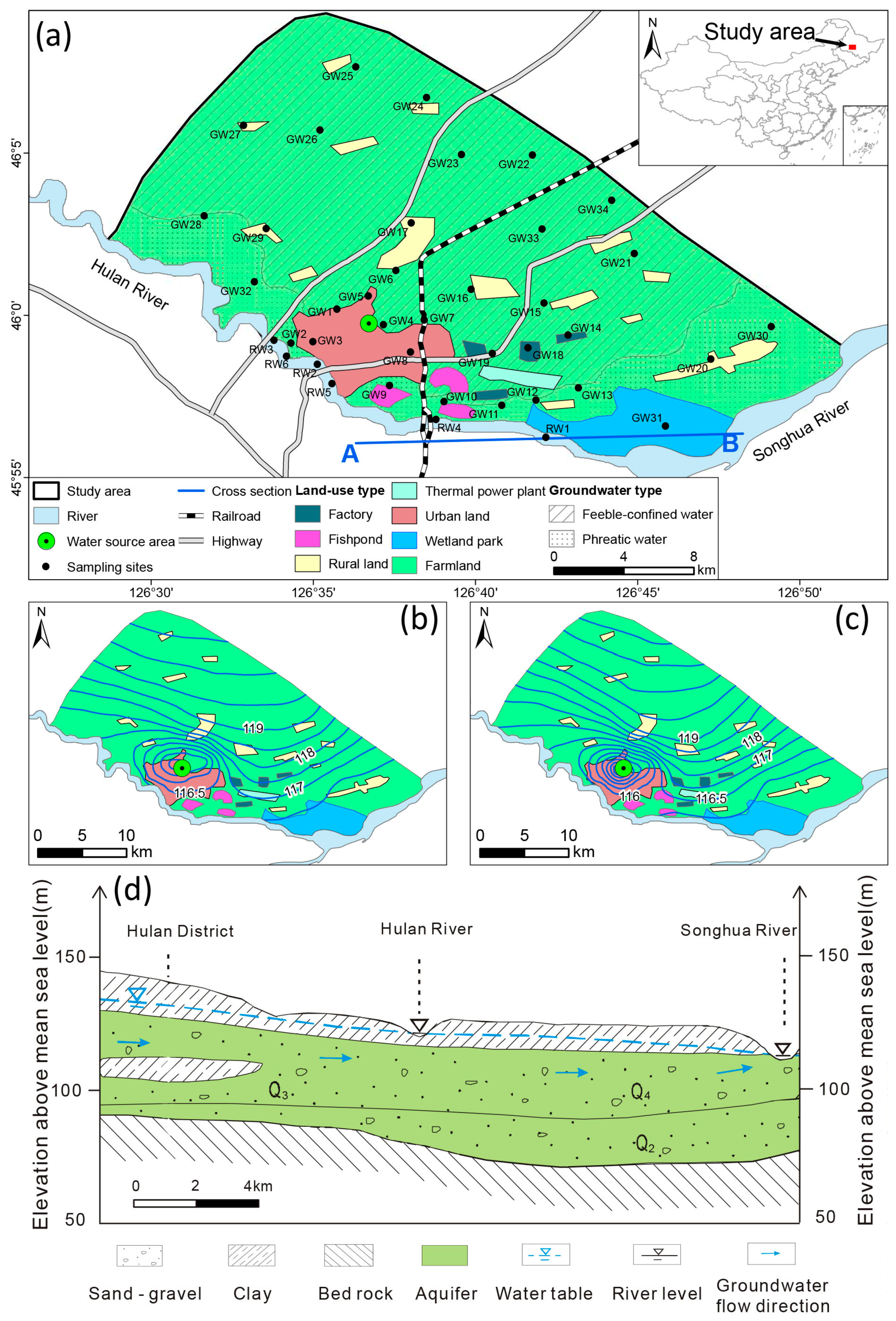
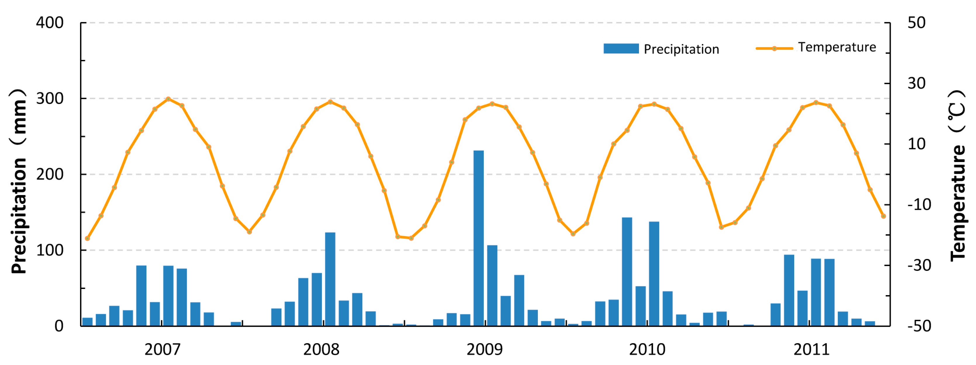
2. Study Area
3. Materials and Methods
3.1. Sample Collection and Analysis
3.2. Principal Component Analysis and Factor Analysis
4. Results and Discussion
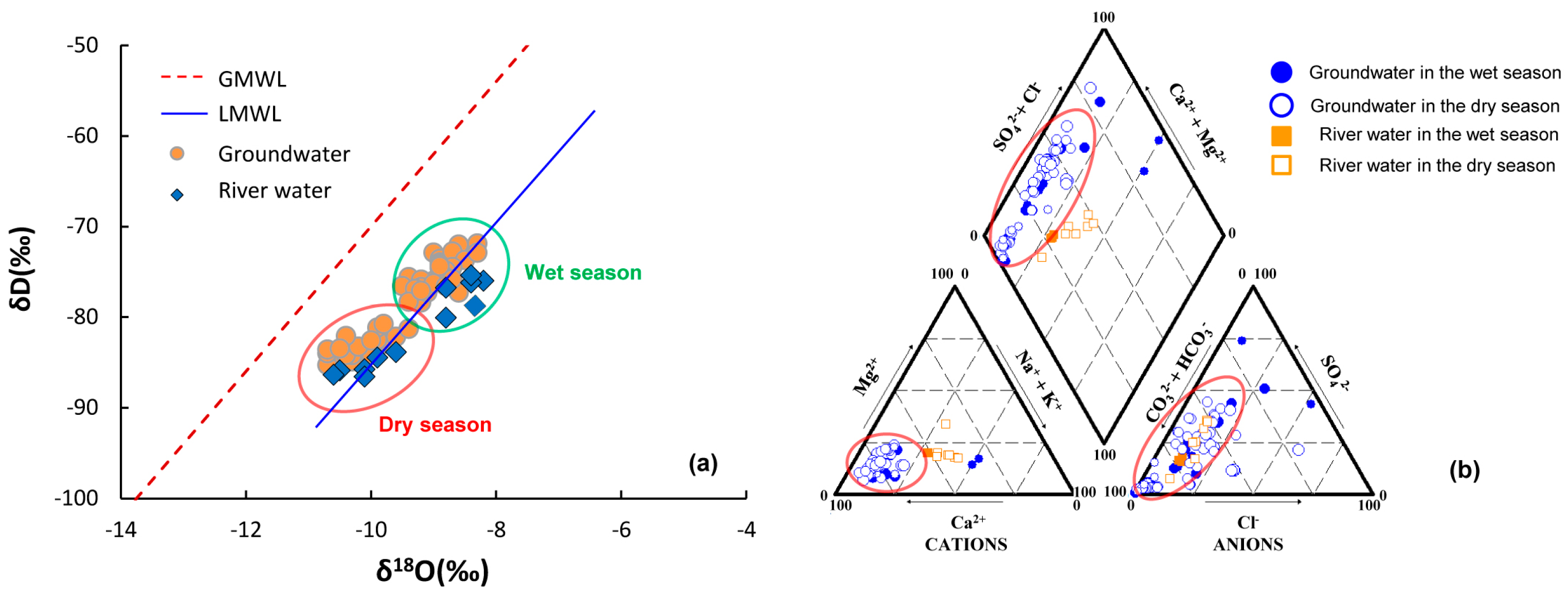
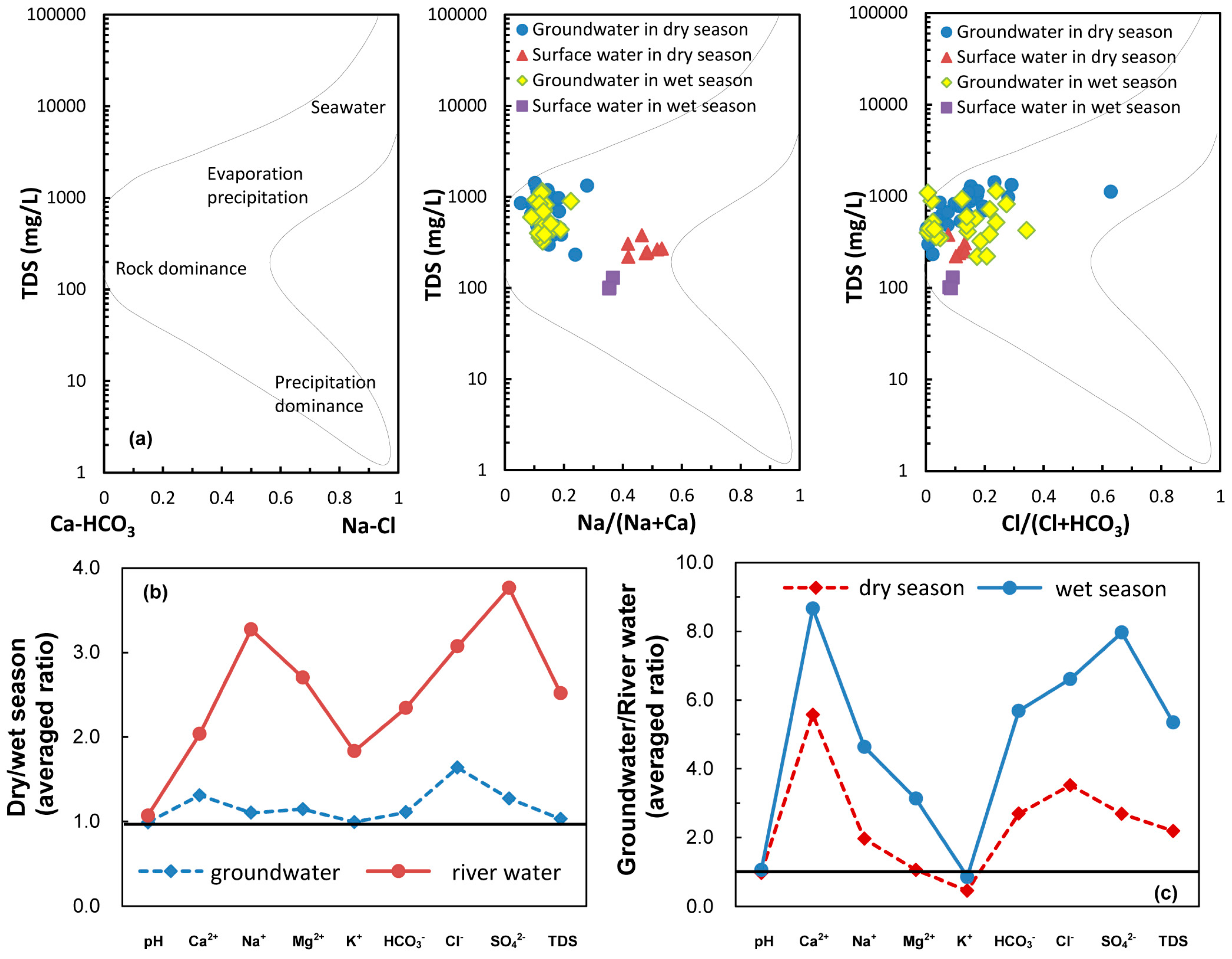
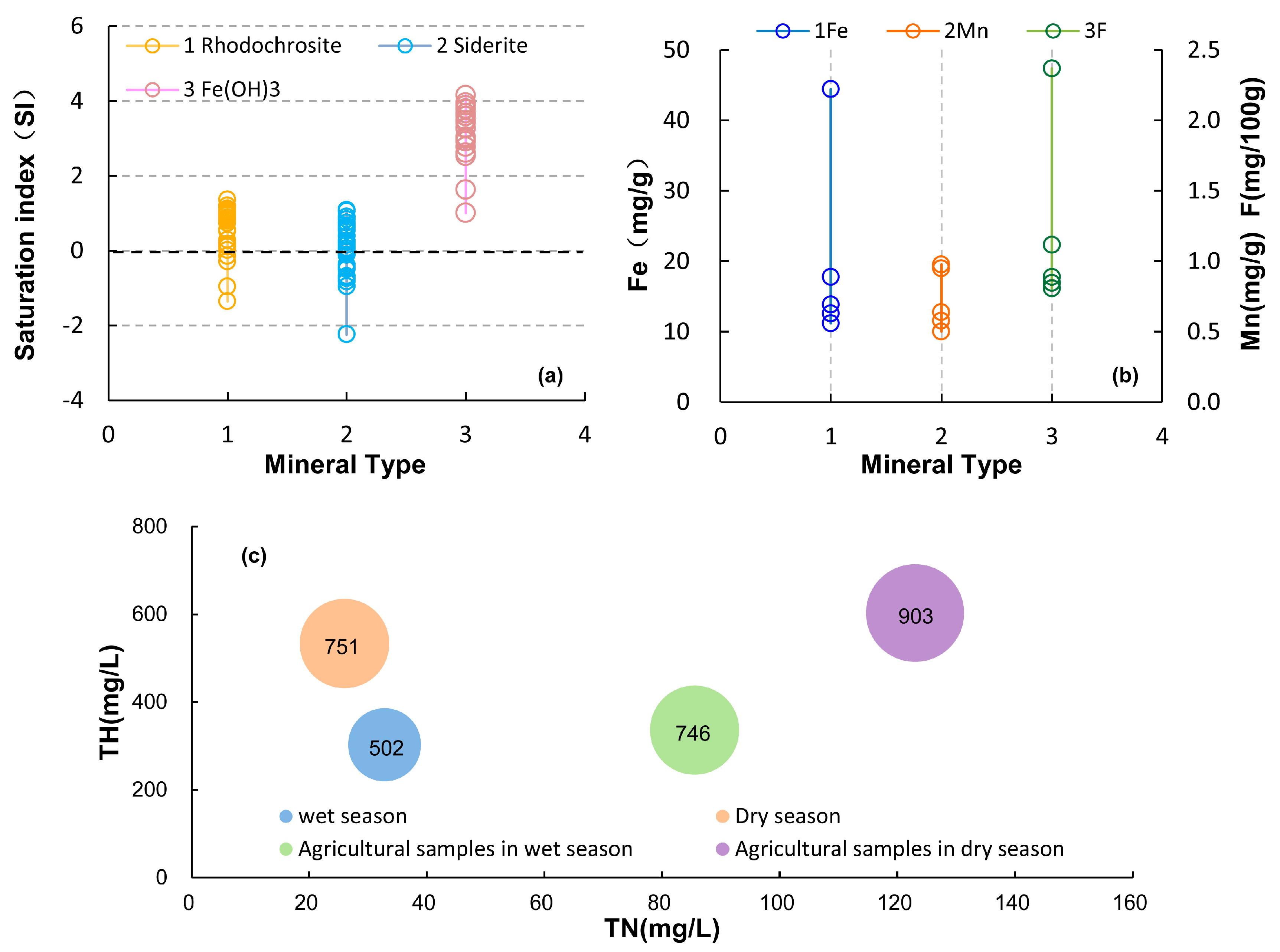
4.1. Water Chemistry
4.2. Source Apportionment of Groundwater Pollution
4.2.1. PCs during the Wet Season (PC-W) and Dry Season (PC-D)
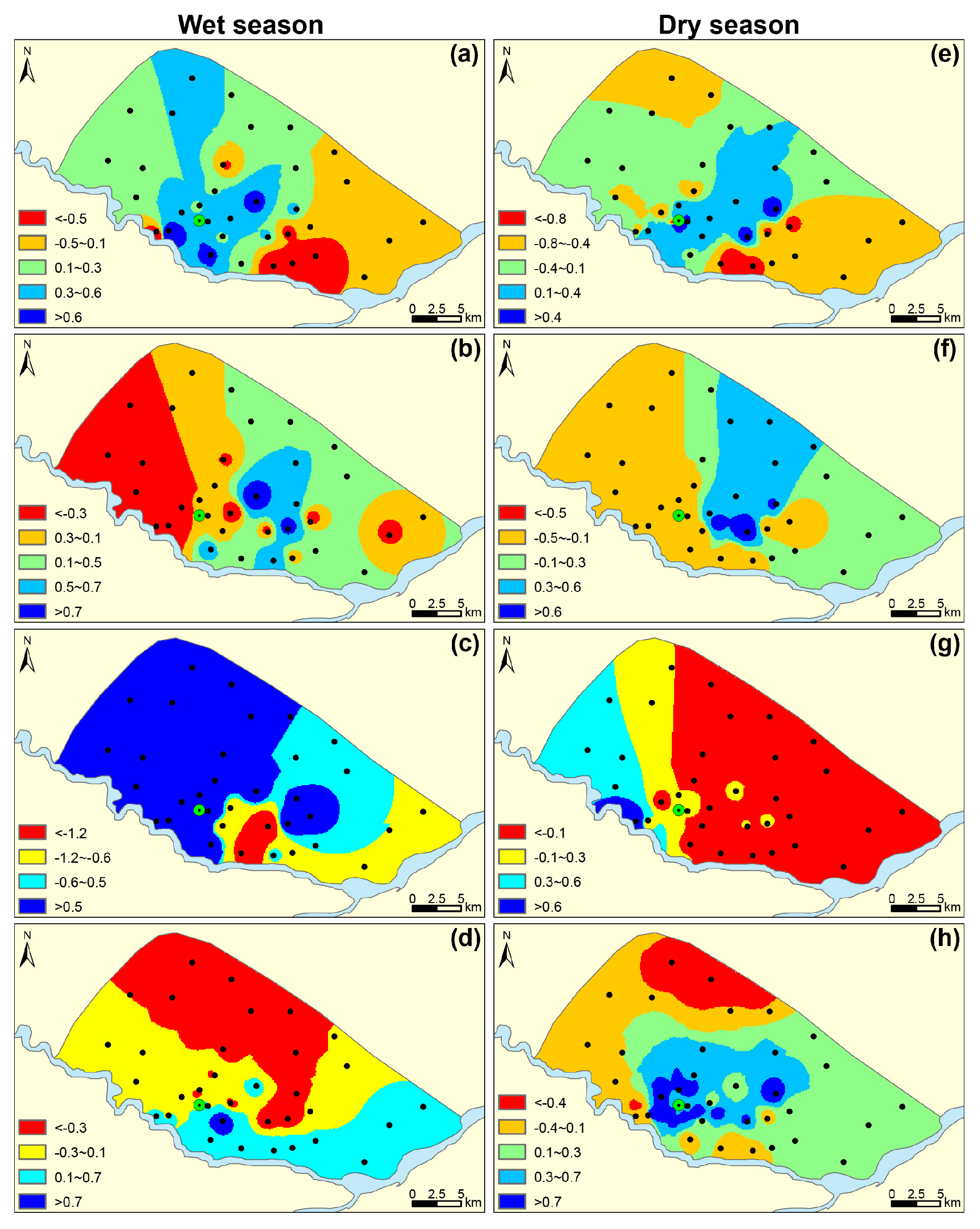
4.2.2. Source Apportionment with Spatial Distribution of PCs
5. Conclusions
Acknowledgments
Author Contributions
Conflicts of Interest
References
- Taylor, R.G.; Scanlon, B.; Döll, P.; Rodell, M.; Beek, R.V.; Wada, Y.; Longuevergne, L.; Leblanc, M.; Famiglietti, J.S.; Edmunds, M. Ground water and climate change. Nat. Clim. Chang. 2013, 3, 322–329. [Google Scholar] [CrossRef] [Green Version]
- MacDonald, A.M.; Bonsor, H.C.; Ahmed, K.M.; Burgess, W.G.; Basharat, M.; Calow, R.C.; Dixit, A.; Foster, S.S.D.; Gopal, K.; Lapworth, D.J.; et al. Groundwater quality and depletion in the indo-gangetic basin mapped from in situ observations. Nat. Geosci. 2016, 9, 762–766. [Google Scholar] [CrossRef]
- Gleeson, T.; Wada, Y.; Bierkens, M.F.; van Beek, L.P. Water balance of global aquifers revealed by groundwater footprint. Nature 2012, 488, 197–200. [Google Scholar] [CrossRef] [PubMed]
- Re, V.; Sacchi, E.; Mas-Pla, J.; Mencio, A.; El Amrani, N. Identifying the effects of human pressure on groundwater quality to support water management strategies in coastal regions: A multi-tracer and statistical approach (Bou-Areg region, Morocco). Sci. Total Environ. 2014, 500–501, 211–223. [Google Scholar] [CrossRef] [PubMed]
- Zeng, X.; Wu, J.; Wang, D.; Zhu, X. Assessing the pollution risk of a groundwater source field at western Laizhou Bay under seawater intrusion. Environ. Res. 2016, 148, 586–594. [Google Scholar] [CrossRef] [PubMed]
- Güler, C.; Kurt, M.A.; Alpaslan, M.; Akbulut, C. Assessment of the impact of anthropogenic activities on the groundwater hydrology and chemistry in tarsus coastal plain (Mersin, SE Turkey) using fuzzy clustering, multivariate statistics and GIS techniques. J. Hydrol. 2012, 414–415, 435–451. [Google Scholar] [CrossRef]
- Sakakibara, K.; Tsujimura, M.; Song, X.; Zhang, J. Spatiotemporal variation of the surface water effect on the groundwater recharge in a low-precipitation region: Application of the multi-tracer approach to the Taihang Mountains, north China. J. Hydrol. 2017, 545, 132–144. [Google Scholar] [CrossRef]
- Menció, A.; Mas-Pla, J. Assessment by multivariate analysis of groundwater-surface water interactions in urbanized Mediterranean streams. J. Hydrol. 2008, 352, 355–366. [Google Scholar] [CrossRef]
- Wang, J.; Liu, R.; Zhang, P.; Yu, W.; Shen, Z.; Feng, C. Spatial variation, environmental assessment and source identification of heavy metals in sediments of the Yangtze river estuary. Mar. Pollut. Bull. 2014, 87, 364–373. [Google Scholar] [CrossRef] [PubMed]
- Shamsuddin, M.K.N.; Sulaiman, W.N.A.; Suratman, S.; Zakaria, M.P.; Samuding, K. Groundwater and surface-water utilisation using a bank infiltration technique in Malaysia. Hydrogeol. J. 2014, 22, 543–564. [Google Scholar] [CrossRef]
- Ascott, M.J.; Lapworth, D.J.; Gooddy, D.C.; Sage, R.C.; Karapanos, I. Impacts of extreme flooding on riverbank filtration water quality. Sci. Total Environ. 2016, 554–555, 89–101. [Google Scholar] [CrossRef] [PubMed]
- Menció, A.; Mas-Pla, J.; Otero, N.; Regàs, O.; Boy-Roura, M.; Puig, R.; Bach, J.; Domènech, C.; Zamorano, M.; Brusi, D. Nitrate pollution of groundwater; all right…, but nothing else? Sci. Total Environ. 2015, 539, 241–251. [Google Scholar] [CrossRef] [PubMed] [Green Version]
- Schuetz, T.; Gascuel-Odoux, C.; Durand, P.; Weiler, M. Nitrate sinks and sources as controls of spatio-temporal water quality dynamics in an agricultural headwater catchment. Hydrol. Earth Syst. Sci. 2016, 20, 843–857. [Google Scholar] [CrossRef]
- Cao, Y.; Tang, C.; Song, X.; Liu, C.; Zhang, Y. Characteristics of nitrate in major rivers and aquifers of the Sanjiang plain, China. J. Environ. Monit. 2012, 14, 2624–2633. [Google Scholar] [CrossRef] [PubMed]
- Thyne, G.; Güler, C.; Poeter, E. Sequential analysis of hydrochemical data for watershed characterization. Groundwater 2004, 42, 711–723. [Google Scholar] [CrossRef]
- Pujari, P.R.; Deshpande, V. Source apportionment of groundwater pollution around landfill site in Nagpur, India. Environ. Monit. Assess. 2005, 111, 43–54. [Google Scholar] [CrossRef] [PubMed]
- Farooqi, A.; Masuda, H.; Firdous, N. Toxic fluoride and arsenic contaminated groundwater in the Lahore and Kasur districts, Punjab, Pakistan and possible contaminant sources. Environ. Pollut. 2007, 145, 839–849. [Google Scholar] [CrossRef] [PubMed]
- Chen, J.; Li, F.; Fan, Z.; Wang, Y. Integrated application of multivariate statistical methods to source apportionment of watercourses in the Liao River Basin, Northeast China. Int. J. Environ. Res. Public Health 2016, 13, 1035–1062. [Google Scholar] [CrossRef] [PubMed]
- Cho, J.C.; Cho, H.B.; Kim, S.J. Heavy contamination of a subsurface aquifer and a stream by livestock wastewater in a stock farming area, Wonju, Korea. Environ. Pollut. 2000, 109, 137–146. [Google Scholar] [CrossRef]
- Tariq, S.R.; Shah, M.H.; Shaheen, N.; Jaffar, M.; Khalique, A. Statistical source identification of metals in groundwater exposed to industrial contamination. Environ. Monit. Assess. 2008, 138, 159–165. [Google Scholar] [CrossRef] [PubMed]
- Li, P.; Wu, J.; Qian, H.; Zhang, Y.; Yang, N.; Jing, L.; Yu, P. Hydrogeochemical characterization of groundwater in and around a wastewater irrigated forest in the southeastern edge of the Tengger desert, Northwest China. Expos. Health 2016, 8, 331–348. [Google Scholar] [CrossRef]
- Rochdane, S.; Reddy, D.V.; El Mandour, A. Hydrochemical and isotopic characterisation of Eastern Haouz plain groundwater, Morocco. Environ. Earth Sci. 2014, 73, 3487–3500. [Google Scholar] [CrossRef]
- Sun, C.; Zhao, W.; Zhang, Q.; Yu, X.; Zheng, X.; Zhao, J.; Lv, M. Spatial distribution, sources apportionment and health risk of metals in topsoil in Beijing, China. Int. J. Environ. Res. Public Health 2016, 13, 727–741. [Google Scholar] [CrossRef] [PubMed]
- Ma, J.; Zhang, W.; Chen, Y.; Zhang, S.; Feng, Q.; Hou, H.; Chen, F. Spatial variability of pahs and microbial community structure in surrounding surficial soil of coal-fired power plants in Xuzhou, China. Int. J. Environ. Res. Public Health 2016, 13, 878–891. [Google Scholar] [CrossRef] [PubMed]
- Chen, H.Y.; Teng, Y.G.; Wang, J.S. Source apportionment for sediment pahs from the Daliao River (China) using an extended fit measurement mode of chemical mass balance model. Ecotoxicol. Environ. Saf. 2013, 88, 148–154. [Google Scholar] [CrossRef] [PubMed]
- Machiwal, D.; Jha, M.K. Identifying sources of groundwater contamination in a hard-rock aquifer system using multivariate statistical analyses and GIS-based geostatistical modeling techniques. J. Hydrol. 2015, 13, 80–110. [Google Scholar] [CrossRef]
- Qin, R.; Wu, Y.; Xu, Z.; Xie, D.; Zhang, C. Assessing the impact of natural and anthropogenic activities on groundwater quality in coastal alluvial aquifers of the Lower Liaohe River plain, NE China. Appl. Geochem. 2013, 31, 142–158. [Google Scholar] [CrossRef]
- Guo, X.; Zuo, R.; Shan, D.; Cao, Y.; Wang, J.; Teng, Y.; Fu, Q.; Zheng, B. Source apportionment of pollution in groundwater source area using factor analysis and positive matrix factorization methods. Hum. Ecol. Risk Assess. 2017, 23, 1417–1436. [Google Scholar] [CrossRef]
- Yao, H.; Qian, X.; Gao, H.; Wang, Y.; Xia, B. Seasonal and spatial variations of heavy metals in two typical chinese rivers: Concentrations, environmental risks, and possible sources. Int. J. Environ. Res. Public Health 2014, 11, 11860–11878. [Google Scholar] [CrossRef] [PubMed]
- The Hulan Water Authority. Planning Report of Groundwater Resources Exploitation and Utilization of Hulan District in Harbin City; The Hulan Water Authority: Harbin, China, 2011. [Google Scholar]
- Zhang, B.; Song, X.; Zhang, Y.; Han, D.; Tang, C.; Yu, Y.; Ma, Y. Hydrochemical characteristics and water quality assessment of surface water and groundwater in Songnen plain, Northeast China. Water Res. 2012, 46, 2737–2748. [Google Scholar] [CrossRef] [PubMed]
- Zhang, B.; Hong, M.; Zhang, B.; Zhang, X.L.; Zhao, Y.S. Fluorine distribution in aquatic environment and its health effect in the western region of the Songnen plain, Northeast China. Environ. Monit. Assess. 2007, 133, 379–386. [Google Scholar] [CrossRef] [PubMed]
- Liu, H.; Jin, G.; Li, J.; Han, J.; Zhang, J.; Guo, D. Determination of stable isotope composition in uranium geological samples. World Nucl. Geosci. 2013, 30, 174–179. (In Chinese) [Google Scholar]
- Craig, H. Isotope variations in meteoric waters. Science 1961, 133, 1702–1703. [Google Scholar] [CrossRef] [PubMed]
- Clark, I.; Fritz, P. Environmental Isotopes in Hydrogeology; CRC Press/Lewis Publishers: Boca Raton, FL, USA, 1997. [Google Scholar]
- Gholizadeh, M.H.; Melesse, A.M.; Reddi, L. Water quality assessment and apportionment of pollution sources using APCS-MLR and PMF receptor modeling techniques in three major rivers of South Florida. Sci. Total Environ. 2016, 566–567, 1552–1567. [Google Scholar] [CrossRef] [PubMed]
- Matiatos, I.; Alexopoulos, A.; Godelitsas, A. Multivariate statistical analysis of the hydrogeochemical and isotopic composition of the groundwater resources in Northeastern Peloponnesus (Greece). Sci. Total Environ. 2014, 476–477, 577–590. [Google Scholar] [CrossRef] [PubMed]
- Standard for Groundwater Quality in China (GB/T 14848-2017). 2017. Available online: http://www.std.gov.cn/ (accessed on 14 October 2017).
- Yang, Q.; Wang, L.; Ma, H.; Yu, K.; Martin, J.D. Hydrochemical characterization and pollution sources identification of groundwater in salawusu aquifer system of Ordos basin, China. Environ. Pollut. 2016, 216, 340–349. [Google Scholar] [CrossRef] [PubMed]
- Gibbs, R.J. Mechanisms controlling world water chemistry. Science 1970, 170, 1088–1090. [Google Scholar] [CrossRef] [PubMed]
- Jeelani, G.; Saravana Kumar, U.; Kumar, B. Variation of δ18O and δD in precipitation and stream waters across the Kashmir Himalaya (India) to distinguish and estimate the seasonal sources of stream flow. J. Hydrol. 2013, 481, 157–165. [Google Scholar] [CrossRef]
- Deng, C. Assessment of the groundwater vulnerability in Harbin and the vicinity. Hydrogeol. Eng. Geol. 2011, 34, 135–139. (In Chinese) [Google Scholar]
- Yuan, L. Hydrochemistry of the groundwater in Songnen plain. Geol. Resour. 2006, 15, 122–125. (In Chinese) [Google Scholar]
- Porowska, D. Determination of the origin of dissolved inorganic carbon in groundwater around a reclaimed landfill in otwock using stable carbon isotopes. Waste Manag. 2015, 39, 216–225. [Google Scholar] [CrossRef] [PubMed]
- Greskowiak, J.; Prommer, H.; Massmann, G.; Johnston, C.D.; Nützmann, G.; Pekdeger, A. The impact of variably saturated conditions on hydrogeochemical changes during artificial recharge of groundwater. Appl. Geochem. 2005, 20, 1409–1426. [Google Scholar] [CrossRef]
- Güler, C. Site characterization and monitoring of natural attenuationindi cator parameters in a fuel contaminated coastal aquifer: Karaduvar (Mersin, Turkey). Environ. Earth Sci. 2009, 59, 631–643. [Google Scholar] [CrossRef]
- Oren, O.; Gavrieli, I.; Burg, A.; Guttman, J.; Lazar, B. Manganese mobilization and enrichment during soil aquifer treatment (SAT) of effluents, the Dan Region Sewage Reclamation Progect (Shafdan), Israel. Environ. Sci. Technol. 2007, 41, 766–772. [Google Scholar] [CrossRef] [PubMed]
- Morgan, J.J. Kinetics of reaction between O2 and Mn(Ⅱ) species in aqueous solutions. Geochim. Cosmochim. Acta 2005, 69, 35–48. [Google Scholar] [CrossRef]
- Petrunic, B.M.; MacQuarrie, K.T.B.; Al, T.A. Reductive dissolution of mn oxides in river-recharged aquifers: A laboratory column study. J. Hydrol. 2005, 301, 163–181. [Google Scholar] [CrossRef]
- Berbenni, P.; Pollice, A.; Canziani, R.; Stabile, L.; Nobili, F. Removal of iron and manganese from hydrocarbon-contaminated groundwater. Bioresour. Technol. 2000, 74, 109–114. [Google Scholar] [CrossRef]
- Ollivier, P.; Surdyk, N.; Azaroual, M.; Besnard, K.; Casanova, J.; Rampnoux, N. Linking water quality changes to geochemical processes occurring in a reactive soil column during treated wastewater infiltration using a large-scale pilot experiment: Insights into Mn behavior. Chem. Geol. 2013, 356, 109–125. [Google Scholar] [CrossRef]
- Marie, A.; Vengosh, A. Source of salinity in groundwater from Jericho area, Jordan Valley. Groundwater 2001, 39, 240–248. [Google Scholar] [CrossRef]
- Kringel, R.; Rechenburg, A.; Kuitcha, D.; Fouepe, A.; Bellenberg, S.; Kengne, I.M.; Fomo, M.A. Mass balance of nitrogen and potassium in urban groundwater in Central Africa, Yaounde/Cameroon. Sci. Total Environ. 2016, 547, 382–395. [Google Scholar] [CrossRef] [PubMed]
- Dzakpasu, M.; Scholz, M.; Harrington, R.; McCarthy, V.; Jordan, S. Groundwater quality impacts from a full-scale integrated constructed wetland. Groundw. Monit. Remediat. 2014, 34, 51–64. [Google Scholar]
- Mamais, D.; Noutsopoulos, C.; Kavallari, I.; Nyktari, E.; Kaldis, A.; Panousi, E.; Nikitopoulos, G.; Antoniou, K.; Nasioka, M. Biological groundwater treatment for chromium removal at low hexavalent chromium concentrations. Chemosphere 2016, 152, 238–244. [Google Scholar] [CrossRef] [PubMed]
- Talalaj, I.A.; Biedka, P. Use of the landfill water pollution index (LWPI) for groundwater quality assessment near the landfill sites. Environ. Sci. Pollut. Res. 2016, 23, 24601–24613. [Google Scholar] [CrossRef] [PubMed]


| Indexes | Min | Max | Mean | Med | S.D | CV | |||||||
|---|---|---|---|---|---|---|---|---|---|---|---|---|---|
| Seasons | WS | DS | WS | DS | WS | DS | WS | DS | WS | DS | WS | DS | |
| GW | pH | 7.06 | 6.91 | 7.97 | 7.94 | 7.68 | 7.58 | 7.78 | 7.60 | 0.31 | 0.29 | 0.04 | 0.04 |
| T | 7.30 | 4.30 | 15.30 | 10.00 | 8.45 | 7.27 | 8.00 | 7.15 | 1.60 | 1.74 | 0.19 | 0.24 | |
| Ca2+ | 18.60 | 46.80 | 265.00 | 298.00 | 137.79 | 180.33 | 153.00 | 170.00 | 2.47 | 72.62 | 0.02 | 0.40 | |
| Mg2+ | 5.28 | 3.96 | 36.60 | 44.30 | 17.34 | 19.84 | 14.20 | 18.45 | 0.75 | 9.94 | 0.04 | 0.50 | |
| Na+ | 15.70 | 12.80 | 54.70 | 96.50 | 27.94 | 30.76 | 17.50 | 26.60 | 0.84 | 19.73 | 0.03 | 0.64 | |
| K+ | 0.56 | 1.22 | 6.50 | 3.47 | 2.04 | 2.02 | 1.54 | 1.95 | 0.25 | 0.64 | 0.12 | 0.31 | |
| HCO3− | 12.30 | 125 | 678.00 | 667.00 | 378.14 | 419.22 | 328.00 | 379.50 | 3.62 | 148.15 | 0.01 | 0.35 | |
| Cl− | 2.10 | 1.31 | 120.00 | 211.00 | 41.53 | 67.93 | 52.90 | 50.40 | 1.45 | 58.83 | 0.04 | 0.87 | |
| SO42− | 3.75 | 9.55 | 318.00 | 289.00 | 95.59 | 121.40 | 138.00 | 122.50 | 2.35 | 75.16 | 0.02 | 0.62 | |
| TDS | 218.00 | 232.00 | 1140.00 | 969.00 | 585.00 | 602.50 | 597.00 | 604.00 | 4.89 | 215.77 | 0.01 | 0.36 | |
| F− | 0.15 | 0.16 | 0.41 | 0.73 | 0.30 | 0.34 | 0.32 | 0.33 | 0.07 | 0.11 | 0.24 | 0.31 | |
| COD | 0.56 | 0.29 | 11.40 | 2.92 | 2.55 | 1.81 | 1.60 | 1.83 | 2.94 | 0.46 | 1.16 | 0.25 | |
| NO3− | 2.14 | 1.19 | 394.00 | 230.00 | 32.40 | 25.34 | 10.33 | 7.60 | 108.58 | 75.09 | 1.90 | 1.67 | |
| NO2− | 0.00 | 0.00 | 1.09 | 0.23 | 0.20 | 0.07 | 0.02 | 0.04 | 0.34 | 0.08 | 1.73 | 1.04 | |
| NH4+ | 0.05 | 0.03 | 5.67 | 1.95 | 0.40 | 0.59 | 0.10 | 0.58 | 1.12 | 0.38 | 2.81 | 0.64 | |
| Fe | 0.03 | 0.02 | 20.70 | 21.20 | 6.53 | 5.20 | 3.33 | 5.63 | 5.92 | 5.32 | 1.14 | 0.81 | |
| Mn | 0.03 | 0.02 | 3.32 | 3.66 | 1.00 | 0.89 | 0.95 | 0.77 | 0.79 | 0.70 | 0.79 | 0.78 | |
| RW | pH | 7.15 | 7.62 | 7.50 | 8.04 | 7.31 | 7.80 | 7.29 | 7.82 | 0.18 | 0.14 | 0.02 | 0.02 |
| T | 26.30 | 2.70 | 28.00 | 8.20 | 27.20 | 5.69 | 27.30 | 5.40 | 0.85 | 1.92 | 0.03 | 0.34 | |
| Ca2+ | 13.90 | 27.10 | 19.50 | 44.70 | 15.90 | 32.36 | 14.30 | 30.30 | 3.12 | 6.65 | 0.20 | 0.21 | |
| Mg2+ | 3.24 | 6.88 | 4.64 | 24.70 | 3.74 | 10.11 | 3.34 | 7.91 | 0.78 | 6.46 | 0.21 | 0.64 | |
| Na+ | 7.60 | 19.50 | 11.30 | 38.80 | 8.93 | 29.20 | 7.88 | 27.50 | 2.06 | 6.57 | 0.23 | 0.23 | |
| K+ | 2.25 | 4.00 | 2.54 | 5.18 | 2.38 | 4.36 | 2.35 | 4.24 | 0.15 | 0.40 | 0.06 | 0.09 | |
| HCO3− | 55.90 | 109.00 | 80.70 | 323.00 | 66.50 | 155.86 | 62.90 | 126.00 | 12.79 | 76.64 | 0.19 | 0.49 | |
| Cl− | 5.22 | 12.50 | 8.12 | 26.90 | 6.28 | 19.30 | 5.50 | 18.20 | 1.60 | 5.38 | 0.25 | 0.28 | |
| SO42− | 11.10 | 22.90 | 13.80 | 68.10 | 12.00 | 45.19 | 11.10 | 39.80 | 1.56 | 16.39 | 0.13 | 0.36 | |
| TDS | 98.00 | 220.00 | 129.00 | 378.00 | 109.33 | 275.43 | 101.00 | 264.00 | 17.10 | 52.5 | 0.16 | 0.1 | |
| F− | 0.21 | 0.22 | 0.26 | 0.61 | 0.23 | 0.35 | 0.22 | 0.33 | 0.03 | 0.13 | 0.12 | 0.36 | |
| COD | 7.52 | 4.14 | 10.30 | 5.94 | 8.91 | 5.13 | 8.91 | 5.10 | 1.97 | 0.59 | 0.22 | 0.12 | |
| NO3− | 3.93 | 5.06 | 4.18 | 6.71 | 4.02 | 14.49 | 4.06 | 5.40 | 0.18 | 0.69 | 0.04 | 0.12 | |
| NO2− | 0.01 | 0.01 | 0.04 | 0.10 | 0.02 | 0.03 | 0.02 | 0.02 | 0.02 | 0.03 | 0.83 | 0.96 | |
| NH4+ | 0.05 | 0.30 | 0.07 | 4.76 | 0.06 | 1.18 | 0.05 | 0.71 | 0.01 | 1.59 | 0.21 | 1.34 | |
| Fe | 0.01 | 0.69 | 2.41 | 3.06 | 1.39 | 1.98 | 1.74 | 1.87 | 1.24 | 0.80 | 0.89 | 0.41 | |
| Mn | 0.07 | 0.14 | 0.13 | 0.22 | 0.10 | 0.19 | 0.10 | 0.21 | 0.03 | 0.03 | 0.29 | 0.18 | |
| Kaiser-Meyer-Olkin Measure of Sampling Adequacy | Wet Season | Dry Season | |
|---|---|---|---|
| 0.511 | 0.547 | ||
| Bartlett’s Test of Sphericity | The approximate chi-square | 1571.422 | 2049.188 |
| Degrees of freedom | 210 | 210 | |
| Significance level | 0 | 0 | |
| Parameters | Components in the Wet Season | Components in the Dry Season | ||||||
|---|---|---|---|---|---|---|---|---|
| PC1-W | PC2-W | PC3-W | PC4-W | PC1-D | PC2-D | PC3-D | PC4-D | |
| K+ | 0.323 | 0.003 | 0.90 | −0.099 | 0.63 | −0.14 | 0.89 | 0.34 |
| Na+ | 0.870 | 0.093 | 0.149 | −0.195 | 0.81 | −0.08 | −0.01 | −0.08 |
| Ca2+ | 0.900 | 0.261 | 0.088 | 0.070 | 0.88 | −0.18 | −0.25 | 0.05 |
| Mg2+ | 0.885 | 0.119 | 0.219 | −0.057 | 0.93 | 0.24 | 0.08 | −0.11 |
| NH4-N | 0.043 | 0.004 | 0.969 | 0.042 | 0.39 | −0.33 | 0.83 | 0.17 |
| HCO3− | 0.820 | −0.341 | 0.411 | −0.090 | 0.11 | 0.21 | 0.49 | 0.23 |
| Cl− | 0.764 | 0.441 | −0.152 | 0.211 | 0.85 | −0.03 | 0.31 | −0.07 |
| SO42− | 0.801 | 0.431 | −0.127 | 0.202 | 0.77 | 0.24 | 0.38 | 0.01 |
| NO3− | −0.158 | 0.261 | 0.777 | −0.172 | 0.35 | 0.01 | 0.84 | 0.03 |
| NO2− | 0.131 | 0.104 | 0.150 | −0.338 | −0.22 | 0.30 | 0.81 | 0.19 |
| Fe | 0.220 | 0.624 | 0.258 | 0.2 | −0.58 | 0.65 | 0.28 | 0.22 |
| Mn | 0.582 | 0.578 | 0.063 | 0.078 | 0.23 | 0.78 | −0.81 | 0.11 |
| F− | 0.471 | −0.795 | −0.085 | 0.072 | 0.10 | 0.32 | 0.43 | 0.84 |
| TH | 0.702 | 0.021 | −0.035 | 0.048 | 0.93 | −0.11 | −0.18 | −0.03 |
| COD | 0.034 | 0.611 | 0.027 | 0.921 | −0.29 | 0.45 | 0.44 | −0.11 |
| TDS | 0.323 | 0.003 | 0.912 | −0.099 | 0.94 | −0.07 | 0.14 | 0.12 |
| Eigenvalue | 6.46 | 3.55 | 1.82 | 1.35 | 6.06 | 3.83 | 2.63 | 1.56 |
| Explained variance (%) | 37.97 | 20.85 | 10.7 | 7.93 | 27.53 | 17.4 | 15.95 | 11.82 |
| Cumulative % of variance | 37.97 | 58.82 | 69.52 | 77.45 | 27.53 | 44.93 | 60.87 | 71.69 |
| Sample NO. | Dry Season | Wet Season | Sample NO. | Dry Season | Wet Season | ||||
|---|---|---|---|---|---|---|---|---|---|
| δ2H | δ18O | δ2H | δ18O | δ2H | δ18O | δ2H | δ18O | ||
| GW1 | −83.4 | −9.9 | −71.9 | −8.3 | GW19 | −84.2 | −10.3 | −74.9 | −8.8 |
| GW2 | −84.7 | −10.6 | −72.9 | −9 | GW20 | −85.3 | −10.7 | −76.7 | −9.2 |
| GW3 | −83.3 | −9.9 | −72.1 | −8.6 | GW21 | −84.2 | −10.3 | −76.6 | −9.5 |
| GW4 | −84.1 | −10.1 | −73.4 | −8.5 | GW22 | −84 | −10.7 | −75.6 | −8.8 |
| GW5 | −84.9 | −10.3 | −72 | −8.6 | GW23 | −81.2 | −9.9 | −72.9 | −8.3 |
| GW6 | −82.6 | −9.8 | −72.9 | −8.7 | GW24 | −84.2 | −10.4 | −74.4 | −8.9 |
| GW7 | −84 | −10 | −73.6 | −8.9 | GW25 | −83.6 | −10.7 | −76.3 | −9 |
| GW8 | −82.9 | −10 | −74 | −8.7 | GW26 | −83.3 | −10.2 | −76.9 | −9.3 |
| GW9 | −83.6 | −10.1 | −74 | −8.9 | GW27 | −78.4 | −9.2 | −77.3 | −8.6 |
| GW10 | −83.8 | −10.5 | −76 | −9 | GW28 | −82.6 | −10 | −78.3 | −9.4 |
| GW11 | −82.5 | −9.9 | −75.6 | −9.4 | GW29 | −82.1 | −10.4 | −77.1 | −9.2 |
| GW12 | −83.3 | −10.1 | −75.9 | −9.2 | GW30 | −83.5 | −10.5 | −76.6 | −8.8 |
| GW13 | −83.8 | −10.3 | −72.8 | −8.7 | RW1 | −85.9 | −10.5 | −79.3 | −7.8 |
| GW14 | −85.1 | −10.6 | −73.7 | −8.5 | RW2 | −83.9 | −9.6 | −76.8 | −8.8 |
| GW15 | −84 | −10.3 | −74.2 | −8.9 | RW3 | −85.8 | −10.1 | −76 | −8.2 |
| GW16 | −82.2 | −9.6 | −74.6 | −8.9 | RW4 | −84.5 | −9.9 | −80.1 | −8.8 |
| GW17 | −84.1 | −10 | −74.5 | −8.7 | RW5 | −86.4 | −10.6 | −76.2 | −8.4 |
| GW18 | −81.3 | −9.4 | −77.3 | −9.1 | RW6 | −86.6 | −10.1 | −75.4 | −8.4 |
© 2018 by the authors. Licensee MDPI, Basel, Switzerland. This article is an open access article distributed under the terms and conditions of the Creative Commons Attribution (CC BY) license (http://creativecommons.org/licenses/by/4.0/).
Share and Cite
Guo, X.; Zuo, R.; Meng, L.; Wang, J.; Teng, Y.; Liu, X.; Chen, M. Seasonal and Spatial Variability of Anthropogenic and Natural Factors Influencing Groundwater Quality Based on Source Apportionment. Int. J. Environ. Res. Public Health 2018, 15, 279. https://doi.org/10.3390/ijerph15020279
Guo X, Zuo R, Meng L, Wang J, Teng Y, Liu X, Chen M. Seasonal and Spatial Variability of Anthropogenic and Natural Factors Influencing Groundwater Quality Based on Source Apportionment. International Journal of Environmental Research and Public Health. 2018; 15(2):279. https://doi.org/10.3390/ijerph15020279
Chicago/Turabian StyleGuo, Xueru, Rui Zuo, Li Meng, Jinsheng Wang, Yanguo Teng, Xin Liu, and Minhua Chen. 2018. "Seasonal and Spatial Variability of Anthropogenic and Natural Factors Influencing Groundwater Quality Based on Source Apportionment" International Journal of Environmental Research and Public Health 15, no. 2: 279. https://doi.org/10.3390/ijerph15020279