Article

Effects of Epiphytes and Depth on Seagrass Spectral Profiles: Case Study of Gulf St. Vincent, South Australia

1
Department of Environmental Engineering, National Cheng Kung Chung University, Tainan City 701, Taiwan
2
Global Water Quality Research Center, National Cheng Kung University, Tainan City 701, Taiwan
3
Department of Ecology & Evolutionary Biology, The University of Adelaide, Adelaide, South Australia 5005, Australia
4
Australian Water Quality Centre, SA Water, Adelaide, South Australia 5000, Australia
5
College of Science and Engineering, Flinders University, Adelaide, South Australia 5001, Australia
*
Authors to whom correspondence should be addressed.
Int. J. Environ. Res. Public Health 2019, 16(15), 2701; https://doi.org/10.3390/ijerph16152701
Submission received: 30 May 2019 / Revised: 20 July 2019 / Accepted: 21 July 2019 / Published: 29 July 2019

Abstract

:
Seagrasses are a crucial indicator species of coastal marine ecosystems that provide substratum, shelter, and food for epiphytic algae, invertebrates, and fishes. More accurate mapping of seagrasses is essential for their survival as a long-lasting natural resource. Before reflectance spectra could properly be used as remote sensing endmembers, factors that may obscure the detection of reflectance signals must be assessed. The objectives in this study are to determine the influence of (1) epiphytes, (2) water depth, and (3) seagrass genus on the detection of reflectance spectral signals. The results show that epiphytes significantly dampen bottom-type reflectance throughout most of the visible light spectrum, excluding 670–679 nm; the depth does influence reflectance, with the detection of deeper seagrasses being easier, and as the depth increases, only Heterozostera increase in the exact “red edge” wavelength at which there is a rapid change in the near-infrared (NIR) spectrum. These findings helped improve the detection of seagrass endmembers during remote sensing, thereby helping protect the natural resource of seagrasses.

1. Introduction

Seagrasses are underwater angiosperms (flowering plants) that tend to form dense beds in shallow, subtidal marine and estuarine benthic seafloors that could be optically clear [1,2,3]. The development and maintained existence of these seagrass beds as a natural resource helps create a substratum and provide shelter, and food sources for epiphytic algae, mollusks, invertebrates, fishes, and sea turtles [4,5,6,7,8]. This, in turn, also allows for the trapping and stabilization of sediments, which helps in maintaining water clarity [1,9,10,11,12]. Because of these effects, seagrasses contribute to the quality of coastal marine ecosystems by improving the biodiversity and productivity within these environments [1,3,13,14,15,16,17,18]. However, although seagrasses are crucial to coastal habitats worldwide, they are in decline, with 29% of the known seagrass areal extent having been lost since 1879 [12,19]. In particular, coastal South Australia has experienced a 21% seagrass reduction [20], with its metropolitan coastal waters undergoing an average annual loss of 85 ha yr−1 until the late 2000s [21,22], with a slow come back in the last decade [23,24,25]. These historical declines emphasize the need for more accurate mapping of seagrasses in the area.
Spectral imaging remote sensing is a proven, useful tool for the detection of seagrass distribution, particularly due to advances in spaceborne and airborne detection sensors [2,26,27,28,29,30]. In particular, since remote sensing spectral reflectances vary along the electromagnetic light spectrum, distinct optical signatures may be repeatedly measured [2,28,31,32,33] with fewer limitations due to cost, time, and inaccessibility [34,35]. Underwater benthic communities, however, are only detected in the visible light spectrum (≈350–750 nm), where light may penetrate the water column without it being readily absorbed and reflected back to a sensor [14,27,36]. Additionally, derivative analyses of hyperspectral data have been used in a number of studies to determine inconspicuous peak features. Although there has been a debate between the use of first-order derivatives [9,37,38,39] compared to second- and fourth-order derivatives [40,41,42,43], the use of these derivatives helps minimize the number of key bandwidths to analyze. In doing so, derivative analyses provide a method to isolate statistically significant spectral differences between benthic bottom types. While baseline knowledge and continual monitoring of seagrass distribution are increasingly critical for mitigation of any further losses, relatively little is known about the factors that may obscure the detection of the reflectance signals such as epiphytes and varying natural growing depths [34,38].
Aquatic epibionts are organisms such as algae, bacteria, sponges, crustaceans, and mollusks that grow on the surface of seagrasses [44,45,46,47]. Note, although the term epiphyte has been defined variously throughout literature [44,45,47,48,49], this paper follows previously extensively reviewed protocol and define an epiphyte as a plant-based epibiont using a plant as a substrate [44]. Nutrient inputs such as nitrate and ammonium promote epiphyte, plankton, and macroalgae growth; thereby, potentially reducing the light that is available for the photosynthetic surfaces of seagrass plants, as well as increasing the drag [50,51]. In general, higher loads of epiphytes are considered detrimental to seagrasses since they reduce growth, cause thinning of shoots, reduce above-ground biomass, and ultimately cause seagrass death [50]. Seagrass complexes (i.e., seagrass and associated epiphytes), however, have been noted to uptake nitrogen from the water column [21]. Posidonia seagrass complexes account for 49–99% of the total biological uptake of nitrate [21], but Amphibolis seagrass complexes have higher uptake rates of ammonium than compared to Posidonia [51]. Seagrasses and their associated epiphytes were estimated to uptake about one-third of all ammonium discharged to the Adelaide region in the mid-2000s, but less than 1% of the nitrate [21].
Generally, the more structurally complex the seagrass, the greater number of epibiont assemblages and a greater degree of epibiont biomass they contain. There is substantial variation in the number of epiphytic algae based on seagrass species [45]. The spatial distribution of epiphytes on seagrass leaves is influenced by the leaf morphology and growth rate [48,52], although the specific side of the leaf, water flow, and canopy height are known to influence epiphyte distribution as well [52]. Due to the basal growth pattern for the strap-shaped leaves of Posidonia [45], the observed trend of epiphyte cover for this seagrass occurs from the base to the tips of the leaves, where the tips of the leaves are older and consequently have a larger amount of time to accumulate epiphytes [51]. For example, 70 taxa of epiphytes have been found in the leaves of Posidonia consisting of diatoms, cyanobacteria, dinoflagellates, red algae, and green algae [53]. Similarly, within the canopies of Amphibolis meadows, epiphytes tended to accumulate in significantly higher biomasses at the tips of the splayed straps of leaf blades [45]. The leaves of certain Amphibolis support larger biomasses of epiphytes comprised of algae and epifaunal grazers than those compared to Posidonia [53]. Conversely, the much smaller size and simpler structure of Zostera and Heterozostera seagrasses have no marked difference in epiphyte abundance based on the spatial distribution of seagrass leaves [45]. However, the effect of epiphytic algae on Heterozostera can vary greatly, with epiphytes contributing from 8% to 49% of the total above-ground biomass in these systems ([45,54], respectively).
Although previous research has been done on epiphytes, there have been limited studies that directly studied the measured changes in the natural growing depth among multiple seagrass genera. Instead, many of these studies primarily focus either on the light availability at extreme depths as a limiting factor, often noting canopy growth [52,55,56,57] or controlled systems with specific incremental depths [9,58]. For example, in a study limited to only Posidonia seagrass, the leaf width and leaf length showed little variability between shallow and deep sites, although there were differences in frond weight and leaf area per shoot [59]. Similarly, in another study of only one benthic type, reflectance responses of the aquatic plant known as Ceratophyllum demersum were measured in a manipulated experiment using a submersible panel and a large, 20,000 L water tank [58]. The results from that study provided a useful reference to the “700 peak”, which is also called the “red edge” due to the rapid change in reflectance within the near-infrared at approximately this waveband.
There is a clear need to understand the influence of epiphytes and varying natural growing depths on the spectral signatures of seagrasses. Specifically, while epiphytes have been shown to affect reflectance responses, the influence of specific seagrass genera is still unclear. In addition to this, there are a limited number of clear and thorough studies of spectral signals from multiple seagrass genera collected from natural growing depths. Therefore, the objectives of this paper are to assess the influence of (1) epiphytes; (2) growing depths, and (3) particular genera on the detection of spectral reflectance signatures of seagrasses.

2. Materials and Methods

2.1. Study Area

The study area is separated into two study sites, Bolivar and Seacliff, which are located north and south along the coasts of metropolitan-Adelaide, South Australia, in the optically shallow waters of Gulf St. Vincent, respectively (Figure 1). The Bolivar research site (34°42′55.82″S, 138°26′45.57″E) is located about 1 km northwest of the outfall of the Bolivar Wastewater Treatment Plant, where Posidonia is the dominant seagrass, followed by a less dense cover of Heterozostera [43,60]. Despite seagrass loss in the area [50], the distribution of these two genera in the northern site has remained consistent for almost a decade [24]. The Seacliff research site (35°2′12.05″ S, 138°30′37.19″ E) is located approximately 0.5 km west of Seacliff Beach, and is dominated by algae and Amphibolis seagrass [60,61]. Posidonia followed by Amphibolis are the dominant seagrass genera in this area, commonly existing as monotypic meadows [62]. Posidonia distribution is more fragmented compared to the northern region [62] due to higher wave energy related to the southern region [63].

2.2. Field Data Collection

Reflectance profiles for the primary submerged aquatic vegetative communities—Posidonia, Amphibolis, and Heterozostera—were collected roughly every 15 days, weather permitting, at the Bolivar and Seacliff study sites during the summer months (Dec. 2015–Jan. 2016). Limiting conditions for accurate measurements for the calculation of reflectance included: taking measurements only when clouds do not obscure the sensor; fractional cloud cover is less than 20%; the least incident shadow from the boat and sensors are being produced; sea state is calm and does not have significant wave height or whitecap fraction; and sea state does not have dominant swell [64,65]. Multiple sites were sampled within these two locations (Figure 1). The specimens were collected by snorkel brought onto the boat. The specimens were selected from areas known to grow largely in homogeneous (monospecific) patches for each particular seagrass. Submerged benthic bottom types were collected at their natural growing depth, and there was no manipulation of depth increments. Not all bottom types were found naturally occurring at all six growing depths investigated (1.1, 1.5, 2.1, 2.4, 2.8, 3.1 m). Once collected, the specimens were sorted by seagrass genera. In-situ downwelling underwater irradiance (Ed in-situ) was measured using a cosine corrector when each time latitude/longitude coordinates were changed.
During the collection of the submerged aquatic vegetation, it was apparent that some specimens were ridden with epiphytes. So when epiphytes were obviously present, seagrass specimens were cut in half soon after they were collected in order to separate the leaf blades from the leaf sheaths. The leaf blades, which are found toward the top of the plant, and the leaf sheaths, which are attached to the rhizomes and roots of the plant, generally represent where epiphytes most frequently and least frequently are found on the seagrass plant, respectively. Uneven sample sizes for each seagrass genera were measured for reflectance from both the leaf blades and leaf sheaths.

2.3. Measuring Spectral Reflectance

Seagrass specimens in the field were then taken to an outdoor laboratory managed by the Australian Water Quality Center to measure for reflectance spectra on cloud-free days within 3 h of solar noon, wherever possible. An open-air 12 L hydraulic vessel was filled with marine water to a depth of 10 cm. After the interior of the vessel was lined in black [41] to minimize wall effects of the light field [26,41,66], specimens were then placed in the vessel. The reflectance for each submerged seagrass sample was determined using a JAZ-2 spectroradiometer [67] sensor. The sensor, which contains a collecting tip with a fiber optic cable (3 m long, 400 μm diameter) for transmission of light, was attached to a CC-3-UV-S cosine corrector [68] and was also mounted to a non-reflective black-colored pole. The cosine corrector is an optical diffuser which couples to the fiber optic cable and spectroradiometer to collect the signal from a field of view that is 180°. Cosine correctors are typically specified for applications requiring the redistribution of the incident light, such as measuring spectral irradiance of a plane surface in air, water, or other media.
Using the mounted pole, the sensor, with its attached fiber optic cable and cosine corrector, was placed just beneath the water surface, and pointed at an angle of ~45° nadir from the specimen sample to record the radiance (≈190–890 nm) in the form of upwelling underwater radiance of a particular benthic bottom type (Eu benthic) and its related upwelling underwater baseline radiance (Eu base). More than 200 spectra were averaged for each representative specimen with an integration time of 10 microseconds; signal-to-noise ratio (SNR) was reported at 250:1 [69].
Reflectance R was calculated using the following equation.
R   benthic =   ( E u   benthic )     ( E u   base ) E d   in - situ
where three variables were measured: upwelling underwater radiance of a specific benthic bottom type (Eu benthic); upwelling underwater radiance of a baseline, in this case as a black-lined vessel (Eu base); and on-site downwelling underwater irradiance (Ed in situ). Data were computed from relative to absolute reflectance by using a Spectralon reference panel; then the spectral database was processed for statistical analyses.

2.4. Statistical Analyses

Before processing could occur, the spectral database at each wavelength was tested for normality. Specifically, data points (∑N > 125,000) were tested with the Shapiro–Wilk test and the Kolmogorov–Smirnov test (p ≥ 0.10, in both cases) for each nanometer. If necessary, data were then normalized; to maintain homoscedasticity, any data points beyond two standard deviations of each one-nanometer increment’s respective median were considered outliers and subsequently removed from further analyses. In most cases, multiple one-way ANOVAs (analyses of variance) were used to statistically analyze the reflectance spectra in order to address the direct effects of epiphyte presence, natural growing depths, and seagrass genera on spectral signatures without producing an unintended interaction factor. Posidonia, Amphibolis, and Heterozostera were found to be naturally growing at 6, 2, and 3 particular depths, respectively; therefore, ANOVA correlation coefficients of first-, second-, and fourth-order derivative reflectance profiles for Amphibolis and Heterozostera were not performed. All analyses were performed using R version 3.2.3 (R Foundation for Statistical Computing, Vienna, Austria).

3. Results and Discussion

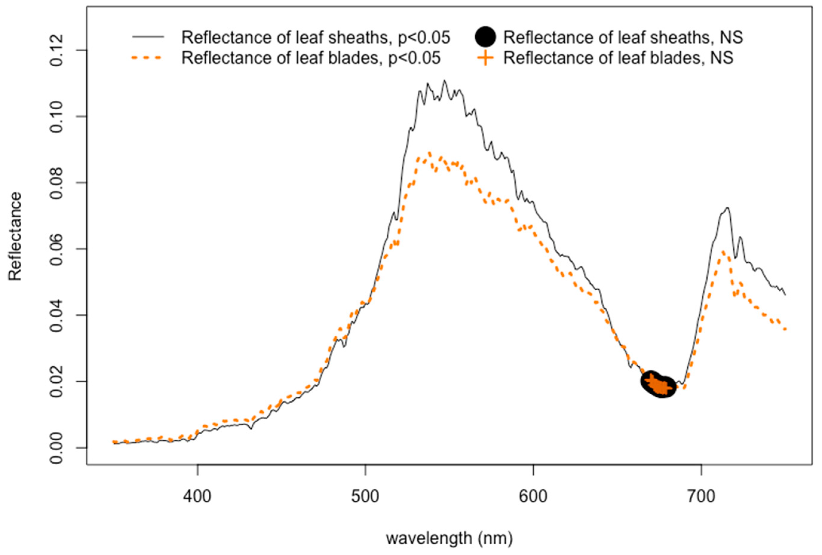
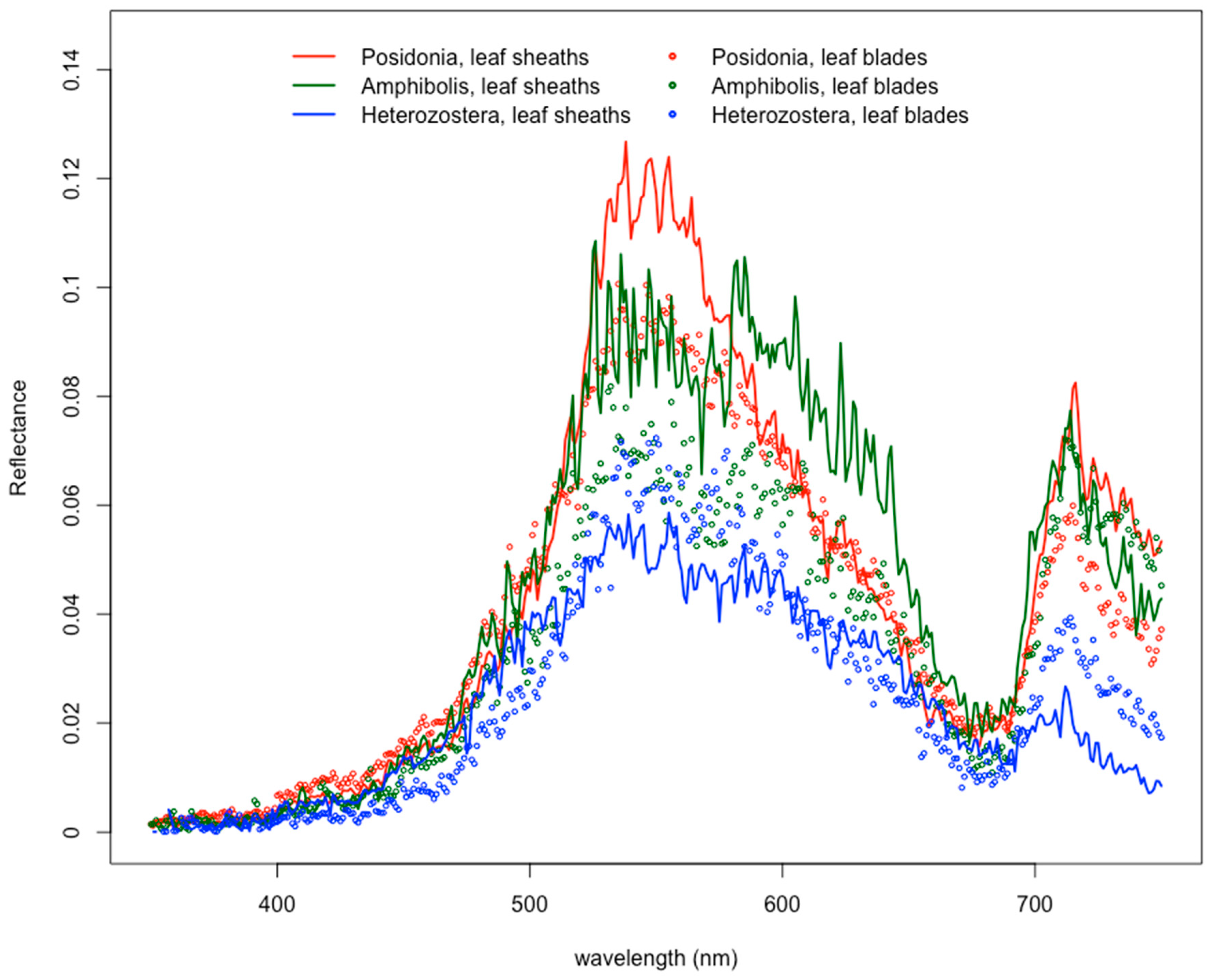
3.1. Epiphytes and the Reflectance Signal

In general, reflectance signals from seagrass leaves were significantly dampened by epiphytes throughout the visible light spectrum, except for one particular bandwidth at 670–679 nm (Figure 2 and Supplementary Materials). The reflectance profiles from the leaf blades of seagrasses, where epiphytes are most frequently attached to the leaf surface, were shown to have significantly lower values than those from the leaf sheath (p < 0.005). This effect also significantly influenced the reflectance values at 566 nm and 600 nm (p < 0.001 for both), thereby potentially weakening the value of the 566:600 band ratio that is used to separate seagrasses from detritus and algae [28,38,70,71]. Epiphytes are known to mask the reflectance of aquatic plant surfaces, which causes altered varying degrees of chl-a absorbance [14]. By competing for the absorbance of photons, especially within the red and blue regions [49], epiphytes thereby contribute their own absorption and reflectance features to the spectral response.
In addition to this, epiphytes, which are inherently chlorophyll-based epibionts, may have a more substantial influence on the reflectance response of seagrasses than constituents within marine water. The results in this study show significant dampening effects of epiphytes attaching directly to the seagrass surface at the leaf blades. At the same time, other studies have shown that measuring the reflectance in filtered and unfiltered marine water has no significant differences throughout most of the visible wavelength spectrum [70,71], suggesting that materials in the water column―including phytoplankton, sediment, minerals, and dissolved organic substances [35,55,72,73]—have less impact on the detection of seagrasses than compared to epiphyte presence on the leaf surface. In spite of the strong dampening influence on the detection of seagrasses, the results in this study show that there is one particular bandwidth at 670–679 nm that disregards the effects of epiphytes.
Beyond this, the 670–679 nm bandwidth discovered in this study can be doubly beneficial for future assessments of seagrasses. Previous research found eleven bandwidths (417, 456, 474, 491, 522, 590, 605, 621, 631, 649, and 681 nm) useful for the differentiation between Posidonia, Amphibolis, and Heterozostera seagrasses [70,71]. Therefore, because this bandwidth falls in the range of one of these eleven bandwidths, isolating and evaluating the reflectance data at approximately 680 nm in a 5 nm increment could be pragmatic and efficient for two reasons. First, first-derivative reflectance could be calculated for the differentiation between seagrasses and other benthic bottom substrates. Second, this bandwidth can still be beneficial to study the differences between seagrasses genera, disregarding the influence of epiphytes. This bandwidth may particularly be useful for future research involving seasonal variations of epiphyte loads where winter months likely allow for less production time of overall chlorophyll, although research in this study involved analyzing spectral reflectance profiles collected during only the summer months.

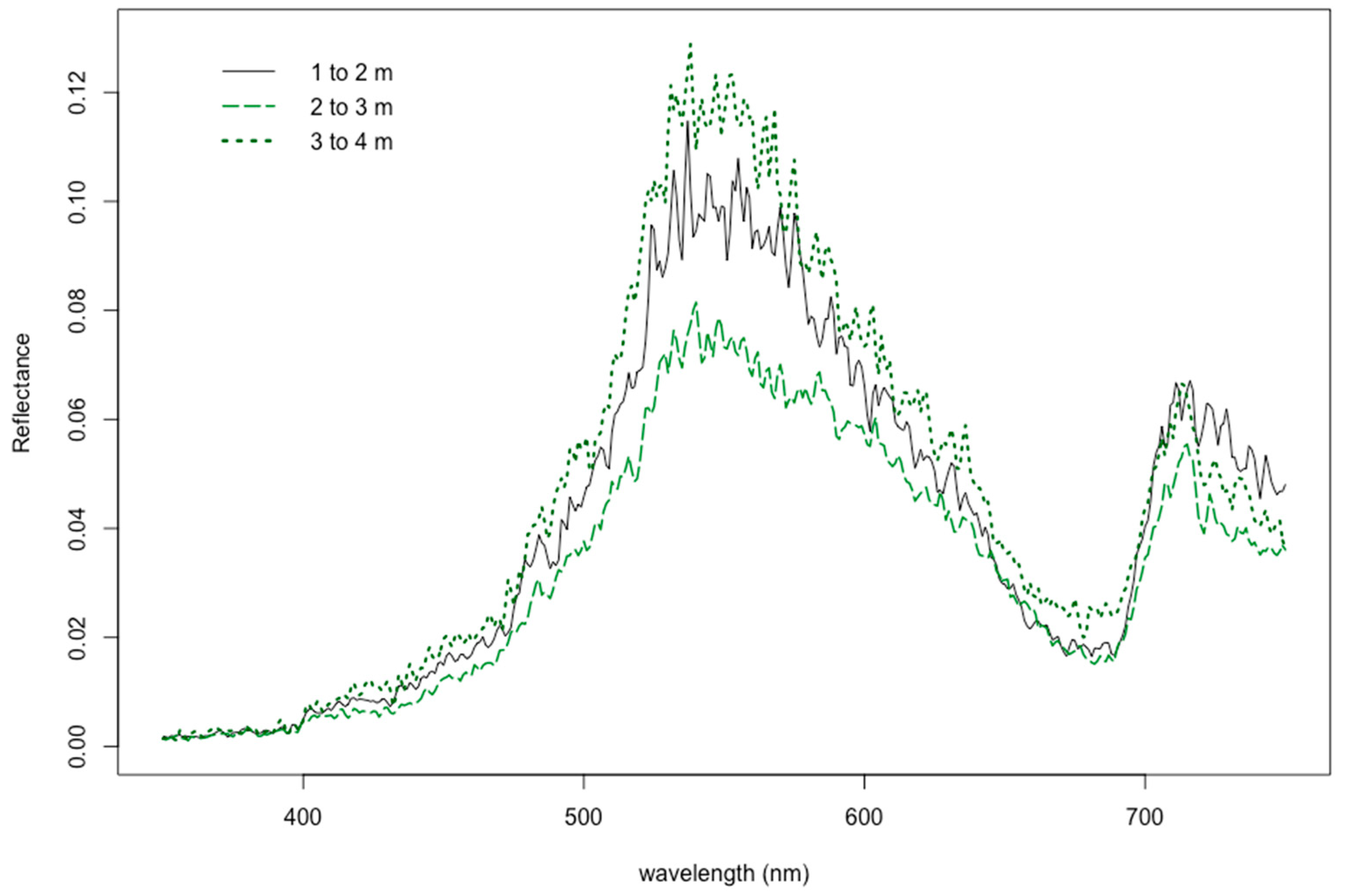
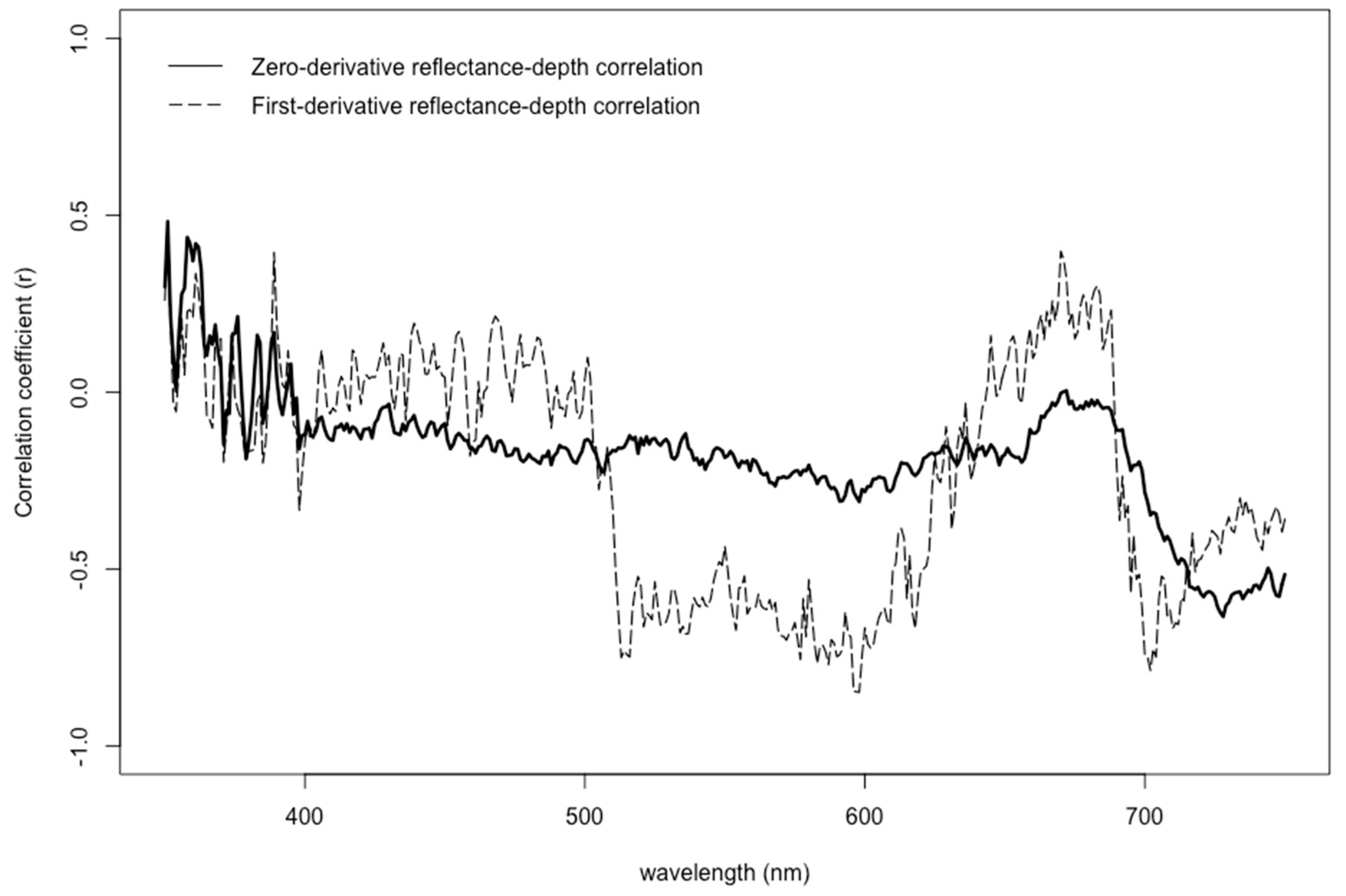
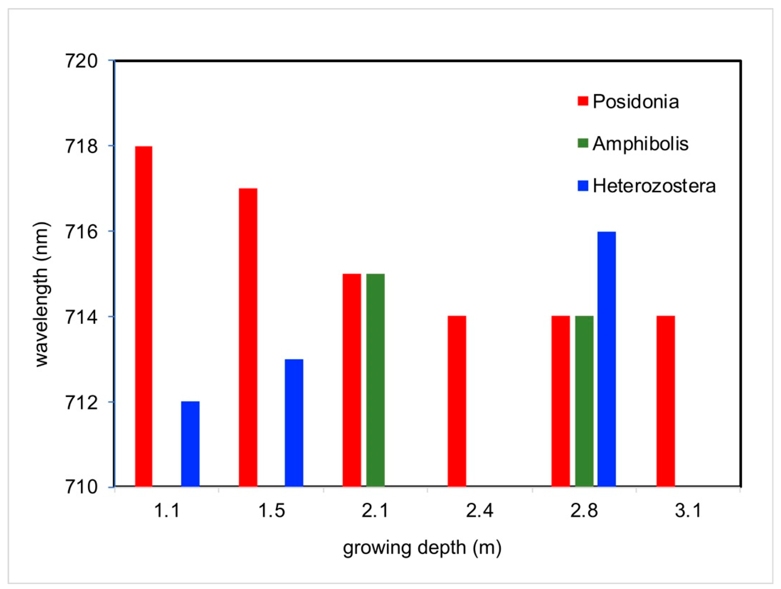
3.2. Reflectance Response due to Natural Growing Depth

Differences in natural growing depths had a significant influence on seagrass spectral response (p < 0.004), with two major trends. First, the reflectance tended to decrease as the depth increased between 1.0–2.0 and 2.0–3.0 m, but in deeper ranges of water depth from 3.0–4.0 m, the reflectance actually increased (Figure 3). Additionally, the correlation of depth to reflectance was also calculated when testing the analyses of variance for original, first-order, second-order, and fourth-order spectral profiles. The original (zero-derivative) spectral profiles generally showed nearly zero correlation from 400–650 nm, and then steadily became increasingly moderately negative correlated (r = −0.55) from 685–730 nm (Figure 4). The first-derivative correlation to growing depth showed two major troughs where three local minima points showed even stronger negative relationships. Specifically, correlation coefficients reached values as low as −0.75, −0.85, and −0.79 at 516, 598, and 702 nm, respectively (Figure 4). The second-order and fourth-order derivative reflectance correlation values were scattered throughout the visible light spectrum, showing no trend whatsoever.
These findings show that the correlation values of first-derivatives with natural growing depth were more strongly negatively correlated than with the zero-derivative profiles, which was similar to other studies [9,58]. Highly correlated features, negative or positive, have been known to help identify [20,37,39,43,74] and potentially eliminate redundant and numerous feature selections for hyperspectral image classification [30,70,71,75], although correlation itself has been noted to help identify only associations rather than causation [9,58,76,77]. Derivative analysis merely finds and sharpens details in spectral curves that are too subtle to notice and hidden within wide zero-order spectrum bands, thereby highlighting features that were already present in direct spectrophotometry [41,78]. Two of these subtle features, in particular, are that 72% and 62% of the variance at 598 and 702 nm are explained by differences in depth (r2 = −0.852 and −0.792), respectively. As a consequence, the results in this study suggest that although the 566:600 and 566:689 band ratios has been shown to be an effective tool for the separation of seagrasses and sand from submerged benthic substrates [35,38,70,71], respectively, these ratios are potentially sensitive to fluctuations in seagrass growing depth. Future research may help identify an alternative feature selection for remote sensing of hyperspectral imagery.
Additionally, the results from the F-value calculations suggest that seagrasses growing in shallower depths are more difficult to detect. Within deeper waters of 2–3 m and 3–4 m, the variances in the reflectance measured from 400–750 nm are sufficiently diverse in range, indicating a greater level of confidence (p < 0.01) for frequent detection and likely differentiation of seagrasses within these deeper growing depths (Figure 5a). Conversely, the F-values of the reflectance profiles of seagrasses growing at 1–2 m show inconsistent bandwidths throughout the visible light spectrum, where there are sufficient levels of confidence (p < 0.05) that they are less easily detected (Figure 5b). These results suggest that reflectance profiles of different vegetative benthic communities may be more difficult to separate in shallower waters.
Detection of different vegetative benthic communities within optically shallow waters must allow for the sea bottom to be visible, where the influence of upwelling underwater radiance signal from seagrass substra can be measured [79]. However varying levels of chlorophyll, suspended matter, and color dissolved organic matter (CDOM) as well as higher wave and wind energy may cause turbid water environments [2,79,80], where the seagrass beds may not be optically clear. Natural growing depth may also be an alternative factor influencing optical clarity [79]. These causes may lead to misclassification of mapping areas with low cover of seagrass, particularly if utilizing a semi-automated [81] or image pre-processing approach [2].
Although the detection of seagrasses in shallower depths may be more difficult, out of eleven previously identified key bandwidths, five can be used with greater confidence in both shallow and deep waters. In a previous study, eleven bandwidths were considered helpful for differentiating between Posidonia, Amphibolis, and Heterozostera seagrasses [70,71]. Five of these key bandwidths—at 417, 456, 522, 590, and 649 nm—fall in the range of bandwidths that have higher levels of confidence for detection (p < 0.01, p < 0.01, p < 0.01, p < 0.01, and p < 0.05, respectively).

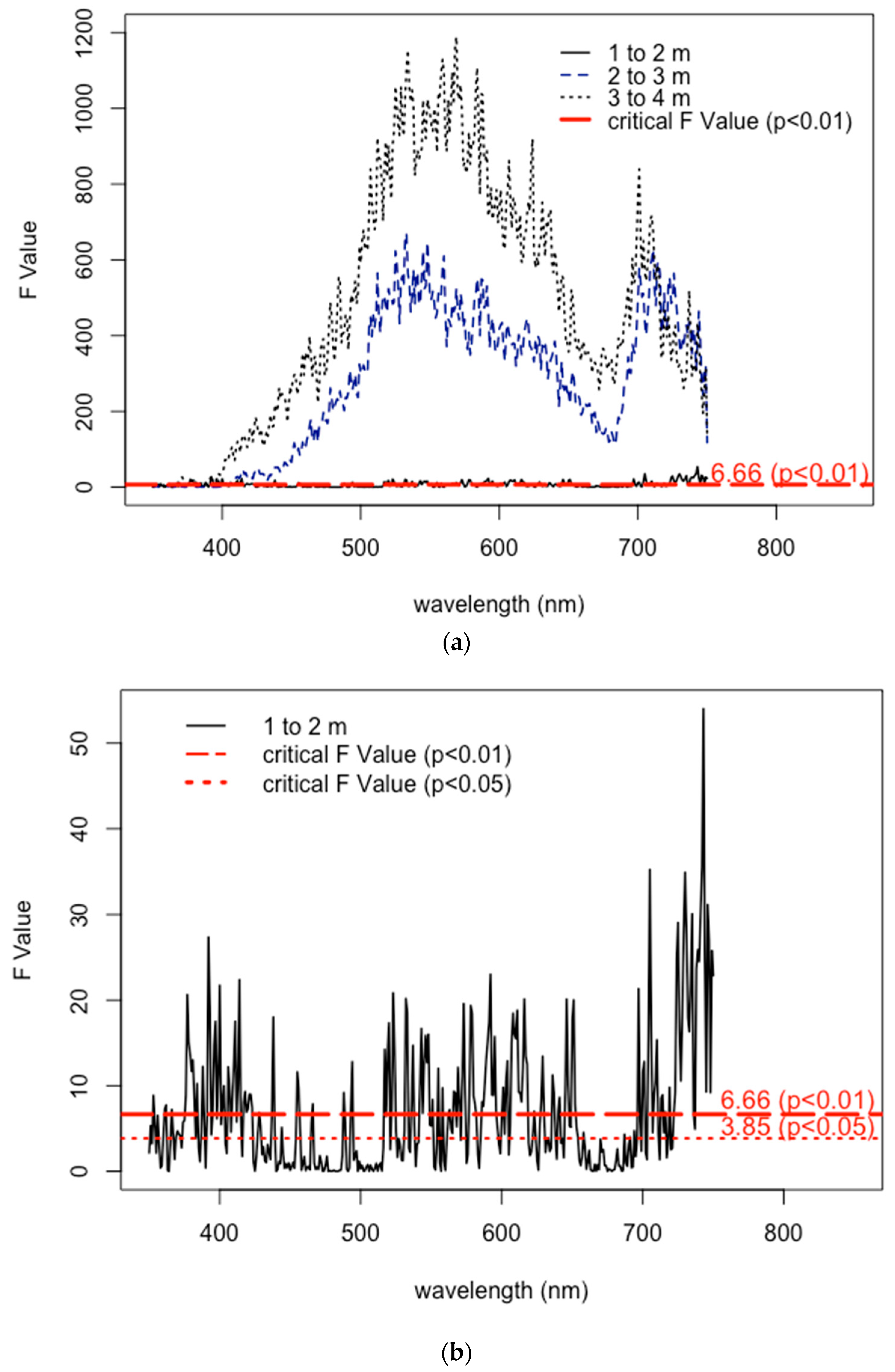
3.3. Epiphyte “Preference” by Seagrass Genus

Although the presence of epiphytes has a dampening effect for each of the seagrasses measured in this study, particular seagrass genera also contribute a significant role in influencing the spectral responses. Specifically, the leaf sheaths at the bottom plant sections of Posidonia and Amphibolis had higher reflectance values than compared to the values at the leaf blades (both p < 0.001); conversely, the reflectance of the leaf blades for Heterozostera had higher reflectance than compared to that of its leaf sheath (p < 0.004) (Figure 6). These differences in spectral responses may be attributed to leaf morphology [48,52] and leaf orientation [28,38,43,49]. Seagrasses containing more flattened leaf morphology tend to have no change in epiphyte community composition, whereas those with curved leaves or leaf bundles supported more diverse epiphyte communities on the concave side [48], potentially creating such distinct microhabitats that few species of epiphytes are common to both stem and leaf [45]. Therefore, results within this study suggest that the epiphytes growing on the wide, long, strap-like leaf blades Posidonia and on the splayed, fan-like leaf blades of Amphibolis had greater advantages for survival and biodiversity than on the shorter, grass-like blades of Heterozostera leaves (Figure 7).

3.4. Influence of Natural Growing Depth on Seagrass Spectral Profiles by Genus

Seagrass genera help to clarify the two major trends observed by the influence of depth on spectral responses. Correlation of original (zero-derivative) spectral profiles and growing depth showed that Posidonia followed a similar trend as previously reported for all seagrasses, with an increasingly negative correlation at around 700 nm (Figure 8). Amphibolis seagrass followed a slightly increased decline in the negative correlation at 700 nm. However, the correlation of Heterozostera increased instead as a positive slope, approaching zero correlation at 700 nm. Posidonia and Amphibolis had negative correlation slopes of −9.1474 × 10⁻³ and −2.1065 × 10⁻³ from 675–725 nm, while Heterozostera instead produced a positive slope of 3.4332 × 10⁻³ within the same bandwidth (Figure 8).
To better understand the phenomena occurring among different seagrass genera, the “700 peak” for each seagrass genera was also assessed at varying water depths. Similar to other findings [9,58], the results in this paper reveal a seagrass genus-specific shift in the exact wavelength at which there is a rapid change of the NIR spectrum. This “700 peak” has been noted to shift to shorter wavelengths in waters that are not optically clear [36,37,38,58,73]. Posidonia and, to a lesser extent, Amphibolis seem to follow the trend that as the natural growing depth of a seagrass increases, the specific wavelength of this shift decreases (Figure 9). This may be attributed to their plasticity and ability to adjust. Posidonia has been known to decouple their light absorption mechanisms to survive the short-term light reduction in deeper water depths due to their larger bodies capable of storing higher quantity and quality of carbohydrates [52].
Heterozostera, however, seemed to show an opposite trend, where the exact wavelength of the 700 peak instead increased as depth increased (Figure 9). This suggests that the 700 peaks for Heterozostera actually shift further in the NIR, potentially making it more difficult for remote sensing detection of submerged aquatic vegetation due to its requirement of being within the visible light spectrum. The results from this study, therefore, show that while Posidonia and Amphibolis are the dominant seagrasses throughout this region, there is increased difficulty for remote sensing of areas where Heterozostera is notably prevalent, such as at the Bolivar Site.

4. Conclusions

In this study, the factors affecting bandwidths for optimal seagrass detection—such as natural growing depth, epiphyte location on the plant, and the potential influence of particular seagrass genera—were assessed. Results in this study reveal the following three major findings. First, while epiphytes tend to dampen reflectance signals throughout the visible light spectrum, the 670–679 bandwidth is not affected by these influences, making it useful for improved detection of submerged aquatic benthic communities. Studying this bandwidth may potentially prove especially useful for future research involving distinguishing nuanced differences based on seasonal variations. Second, natural growing depth influences the spectral responses of benthic bottom types, making the detection of seagrasses growing within 1–2 m more difficult than the detection of those growing in deeper water depths of 2–3 and 3–4 m. However, five particular bandwidths known to differentiate between Posidonia, Amphibolis, and Heterozostera—417, 456, 522, 590, and 649 nm—could be used with higher levels of confidence for the detection of seagrasses in shallower and deeper waters. Third, the genus of a particular seagrass plays a role in influencing the “700 peak”, that is, where there is a rapid change of the NIR spectrum. The detection of Heterozostera in deeper waters may be more difficult since remote sensing of underwater communities can only be detected within the visible light spectrum. The findings in this study may be used to improve detection of benthic community substrates during remote sensing and monitoring of seagrass distribution. In doing so, submerged aquatic vegetation within coastal environments can be managed more thoroughly and more frequently, thereby mitigating potential anthropogenic impacts and protecting seagrasses as a natural resource.

Supplementary Materials

The following are available online at https://www.mdpi.com/1660-4601/16/15/2701/s1.

Author Contributions

M.B., M.F. and C.-H.C. suggested and supervised the conceptualization of the research. T.K. conceived and designed the experiment; C.H. and T.K. troubleshooted, redesigned, and performed the experiments. C.H. processed and analyzed the acquired data. C.H. drafted the current paper; M.B., M.F., T.K., and C.H. edited the paper.

Funding

This research was funded in part by a research grant (Research Project No. CS7665) provided through the 2012–2013 Premier’s Research and Industry Fund (PRIF), a part of the Department of Further Education, Employment, Science, and Technology (DFEEST), Government of South Australia, Australia. C. Hwang was supported by funding from National Cheng Kung University (NCKU) Distinguished International Student Scholarship, NCKU Dept. of Engineering International Student Scholarship, NCKU Dept. of Engineering Research Assistantship, and CTCI Foundation Scholarship for Overseas Graduate Students.

Acknowledgments

The authors express their gratitude to G. Westphalen, A. Mussared, L. VanDerLinden, R. Daly, and the rest of the staff at Australian Water Quality Centre, SA Water, Adelaide, South Australia, Australia for assistance with fieldwork and data analyses.

Conflicts of Interest

The authors declare no conflict of interest.

References

  1. Hemminga, M.A.; Duarte, C.M. Seagrass Ecology; Cambridge University Press: Cambridge, UK, 2008; p. 312. [Google Scholar]
  2. Phinn, S.; Roelfsema, C.; Dekker, A.; Brando, V.; Anstee, J.; Brando, V. Mapping seagrass species, cover and biomass in shallow waters: An assessment of satellite multi-spectral and airborne hyper-spectral imaging systems in Moreton Bay (Australia). Remote Sens. Environ. 2008, 112, 3413–3425. [Google Scholar] [CrossRef]
  3. Williams, S.L.; Heck, K.L., Jr. Seagrass community ecology. In Marine Community Ecology; Bertness, M.D., Gaines, S.D., Hay, M.E., Eds.; Sinauer Associates, Inc.: Sunderland, MA, USA, 2011; pp. 317–337. [Google Scholar]
  4. Fourqurean, J.; Manuel, S.; Coates, K.; Kenworthy, W.; Smith, S. Effects of excluding sea turtle herbivores from a seagrass bed: Overgrazing may have led to loss of seagrass meadows in Bermuda. Mar. Ecol. Prog. Ser. 2010, 419, 223–232. [Google Scholar] [CrossRef] [Green Version]
  5. Cappello, T.; Giannetto, A.; Parrino, V.; Maisano, M.; Oliva, S.; De Marco, G.; Guerriero, G.; Mauceri, A.; Fasulo, S. Baseline levels of metabolites in different tissues of mussel Mytilus galloprovincialis (Bivalvia: Mytilidae). Comp. Biochem. Physiol. Part D Genom. Proteom. 2018, 26, 32–39. [Google Scholar] [CrossRef]
  6. Esteban, N.; Unsworth, R.; Gourlay, J.; Hays, G. The discovery of deep-water seagrass meadows in a pristine Indian Ocean wilderness revealed by tracking green turtles. Mar. Pollut. Bull. 2018, 134, 99–105. [Google Scholar] [CrossRef]
  7. Fourqurean, J.W.; Manuel, S.A.; Coates, K.A.; Massey, S.C.; Kenworthy, W.J. Decadal Monitoring in Bermuda Shows a Widespread Loss of Seagrasses Attributable to Overgrazing by the Green Sea Turtle Chelonia mydas. Estuaries Coasts 2019, 1–17. [Google Scholar] [CrossRef]
  8. Parrino, V.; Costa, G.; Cannavà, C.; Fazio, E.; Bonsignore, M.; Concetta, S.; Piccione, G.; Fazio, F. Flow cytometry and micro-Raman spectroscopy: Identification of hemocyte populations in the mussel Mytilus galloprovincialis (Bivalvia: Mytilidae) from Faro Lake and Tyrrhenian Sea (Sicily, Italy). Fish Shellfish Immunol. 2019, 87, 1–8. [Google Scholar] [CrossRef]
  9. Han, L. Spectral reflectance of Thalassia testudinum with varying depths. In Proceedings of the International Geoscience and Remote Sensing Symposium, Toronto, ON, Canada, 24–28 June 2002; pp. 2123–2125. [Google Scholar]
  10. Dierssen, H.M.; Zimmerman, R.C.; Leathers, R.A.; Downes, T.V.; Davis, C.O. Ocean color remote sensing of seagrass and bathymetry in the Bahamas Banks by high-resolution airborne imagery. Limnol. Oceanogr. 2003, 48, 444–455. [Google Scholar] [CrossRef]
  11. Orth, R.J.; Carruthers, T.J.B.; Dennison, W.C.; Duarte, C.M.; Fourqurean, J.W.; Heck, K.L.; Hughes, A.R.; Kendrick, G.A.; Kenworthy, W.J.; Olyarnik, S.; et al. A Global Crisis for Seagrass Ecosystems. Bioscience 2006, 56, 987–996. [Google Scholar] [CrossRef] [Green Version]
  12. Barbier, E.B.; Hacker, S.D.; Kennedy, C.; Koch, E.W.; Stier, A.C.; Silliman, B.R. The value of estuarine and coastal ecosystem services. Ecol. Monogr. 2011, 81, 169–193. [Google Scholar] [CrossRef]
  13. Duarte, C.M. The future of seagrass meadows. Environ. Conserv. 2002, 29, 192–206. [Google Scholar] [CrossRef] [Green Version]
  14. Fyfe, S.K. Spatial and temporal variation in spectral reflectance: Are seagrass species spectrally distinct? Limnol. Oceanogr. 2003, 48, 464–479. [Google Scholar] [CrossRef]
  15. Wabnitz, C.C.; Andréfouët, S.; Torres-Pulliza, D.; Müller-Karger, F.E.; Kramer, P.A. Regional-scale seagrass habitat mapping in the Wider Caribbean region using Landsat sensors: Applications to conservation and ecology. Remote Sens. Environ. 2008, 112, 3455–3467. [Google Scholar] [CrossRef]
  16. Dolch, T.; Reise, K. Long-term displacement of intertidal seagrass and mussel beds by expanding large sandy bedforms in the northern Wadden Sea. J. Sea Res. 2010, 63, 93–101. [Google Scholar] [CrossRef] [Green Version]
  17. Borfecchia, F.; De Cecco, L.; Martini, S.; Ceriola, G.; Bollanos, S.; Vlachopoulos, G.; Valiante, L.M.; Belmonte, A.; Micheli, C. Posidonia oceanica genetic and biometry mapping through high-resolution satellite spectral vegetation indices and sea-truth calibration. Int. J. Remote Sens. 2013, 34, 4680–4701. [Google Scholar] [CrossRef]
  18. Cunha, A.H.; Assis, J.F.; Serrão, E.A. Reprint of “Seagrasses in Portugal: A most endangered marine habitat. Aquat. Bot. 2014, 115, 3–13. [Google Scholar] [CrossRef]
  19. Waycott, M.; Duarte, C.M.; Carruthers, T.J.B.; Orth, R.J.; Dennison, W.C.; Olyarnik, S.; Calladine, A.; Fourqurean, J.W.; Heck, K.L.; Hughes, A.R.; et al. Accelerating loss of seagrasses across the globe threatens coastal ecosystems. Proc. Natl. Acad. Sci. USA 2009, 106, 12377–12381. [Google Scholar] [CrossRef] [Green Version]
  20. Blackburn, D.T.; Dekker, A.G. Remote Sensing Study of Marine and Coastal Features and Interpretation of Changes in Relation to Natural and Anthropogenic Processes: Final Technical Report; ACWS Technical Report No. 6. Prepared for the Adelaide Coastal Waters Study Steering Committee; South Australian Environment Protection Authority (SA EPA): Adelaide, Australia, 2006.
  21. Nayar, S.; Collings, G.; Pfennig, P.; Royal, M. Managing nitrogen inputs into seagrass meadows near a coastal city: Flow-on from research to environmental improvement plans. Mar. Pollut. Bull. 2012, 64, 932–940. [Google Scholar] [CrossRef]
  22. Tanner, J.E.; Irving, A.D.; Fernandes, M.; Fotheringham, D.; McArdle, A.; Murray-Jones, S.; Murray-Jones, S. Seagrass rehabilitation off metropolitan Adelaide: A case study of loss, action, failure and success. Ecol. Manag. Restor. 2014, 15, 168–179. [Google Scholar] [CrossRef]
  23. Hart, D. Seagrass Extent Change 2007-13-Adelaide Coastal Waters; DEWNR Technical Note 2013/07; Government of South Australia, Department of Environment Water and Natural Resources: Adelaide, Australia, 2013; p. 19.
  24. Tanner, J.E.; Theil, M.; Fotheringham, D.G. Seagrass Condition Monitoring: Encounter Bay and Port Adelaide; Final Report Prepared for the Adelaide and Mount Lofty Ranges Natural Resources Management Board. SARDI Publication No. F2012/000139-2. SARDI Research Report Series No. 799; Theil, M., Ed.; South Australian Research and Development Institution: West Beach, Australia, 2014.
  25. Clarke, K.; Hennessy, A.; Lewis, M. Adelaide Metropolitan Coastline Benthic Habitat Mapping from Hyperspectral Imagery; Product A: Bare-Substrate vs Non-Bare Substrate. Prepared for SA Water, SA Department for Environment and Water, and SA Environmental Protection Authority, School of Biological Sciences, The University of Adelaide, Adelaide, South Australia; The University of Adelaide: Adelaide, Australia, 2018. [Google Scholar]
  26. Dunk, I.; Lewis, M. Seagrass and shallow water feature discrimination using HyMap imagery. In Proceedings of the 10th Australasian Remote Sensing Photogrammetry Conference, Adelaide, Australia, 21–25 August 2000. [Google Scholar]
  27. Brando, V.; Dekker, A. Satellite hyperspectral remote sensing for estimating estuarine and coastal water quality. IEEE Trans. Geosci. Remote Sens. 2003, 41, 1378–1387. [Google Scholar] [CrossRef]
  28. O’Neill, J.D.; Costa, M. Mapping eelgrass (Zostera marina) in the Gulf Islands National Park Reserve of Canada using high spatial resolution satellite and airborne imagery. Remote Sens. Environ. 2013, 133, 152–167. [Google Scholar] [CrossRef]
  29. Kakuta, S.; Takeuchi, W.; Prathep, A. Seaweed and seagrass mapping in Thailand measured by using Landsat 8 optical and texture properties. In Proceedings of the International Symposium on Remote Sensing (ISRS), Tainan, Taiwan, 22–24 April 2015. [Google Scholar]
  30. Medjahed, S.A.; Ouali, M. Band selection based on optimization approach for hyperspectral image classification. Egypt. J. Remote Sens. Space Sci. 2018, 21, 413–418. [Google Scholar] [CrossRef]
  31. Vahtmäe, E.; Kutser, T.; Martin, G.; Kotta, J. Feasibility of hyperspectral remote sensing for mapping benthic macroalgal cover in turbid coastal waters—A Baltic Sea case study. Remote Sens. Environ. 2006, 101, 342–351. [Google Scholar] [CrossRef]
  32. Chang, C.-H.; Liu, C.-C.; Chung, H.-W.; Lee, L.-J.; Yang, W.-C. Development and evaluation of a genetic algorithm-based ocean color inversion model for simultaneously retrieving optical properties and bottom types in coral reef regions. Appl. Opt. 2014, 53, 605–617. [Google Scholar] [CrossRef]
  33. Veys, C.; Hibbert, J.; Davis, P.; Grieve, B. An ultra-low-cost active multispectral crop diagnostics device. In Proceedings of the 2017 IEEE SENSORS, Glasgow, UK, 29 October–1 November 2017. [Google Scholar]
  34. Dekker, A.G.; Brando, V.E.; Anstee, J.M. Retrospective seagrass change detection in a shallow coastal tidal Australian lake. Remote Sens. Environ. 2005, 97, 415–433. [Google Scholar] [CrossRef]
  35. Dekker, A.; Brando, V.; Anstee, J.; Fyfe, S.; Malthus, T.; Karpouzli, E. Remote Sensing of Seagrass Ecosystems: Use of Spaceborne and Airborne Sensors. In Seagrasses: Biology, Ecology and Conservation; Springer: Dordrecht, The Netherlands, 2006; pp. 347–359. [Google Scholar]
  36. Mumby, P.J.; Skirving, W.; Strong, A.E.; Hardy, J.T.; LeDrew, E.F.; Hochberg, E.J.; Stumpf, R.P.; David, L.T. Remote sensing of coral reefs and their physical environment. Mar. Pollut. Bull. 2004, 48, 219–228. [Google Scholar] [CrossRef]
  37. Karpouzli, E.; Malthus, T.J.; Place, C.J. Hyperspectral discrimination of coral reef benthic communities in the western Caribbean. Coral Reefs 2004, 23, 141–151. [Google Scholar] [CrossRef]
  38. O’Neill, J.D.; Costa, M.; Sharma, T. Remote Sensing of Shallow Coastal Benthic Substrates: In situ Spectra and Mapping of Eelgrass (Zostera marina) in the Gulf Islands National Park Reserve of Canada. Remote Sens. 2011, 3, 975. [Google Scholar] [CrossRef]
  39. Fulton, S. An analysis of the spectral reflectance separability of Amphibolis griffithii and Posidonia sinuosa at different water depths. In School of the Environment; The Flinders University of South Australia: Adelaide, Australia, 2014; p. 97. [Google Scholar]
  40. Tsai, F.; Philpot, W. Derivative Analysis of Hyperspectral Data. Remote Sens. Environ. 1998, 66, 41–51. [Google Scholar] [CrossRef]
  41. Hochberg, E.J.; Atkinson, M.J. Spectral discrimination of coral reef benthic communities. Coral Reefs 2000, 19, 164–171. [Google Scholar] [CrossRef]
  42. Bargain, A.; Robin, M.; Le Men, E.; Huete, A.; Barillé, L. Spectral response of the seagrass Zostera noltii with different sediment backgrounds. Aquat. Bot. 2012, 98, 45–56. [Google Scholar] [CrossRef]
  43. Bargain, A.; Robin, M.; Méléder, V.; Rosa, P.; le Menn, E.; Harin, N.; Barillé, L. Seasonal spectral variation of Zostera noltii and its influence on pigment-based Vegetation Indices. J. Exp. Mar. Biol. Ecol. 2013, 446, 86–94. [Google Scholar] [CrossRef]
  44. Taylor, P.; Wilson, M. Palaeoecology and evolution of marine hard substrate communities. Earth Sci. Rev. 2003, 62, 1–103. [Google Scholar] [CrossRef]
  45. Borowitzka, M.A.; Lavery, P.S.; van Keulen, M. Epiphytes of Seagrasses. In Seagrasses: Biology, Ecology and Conservation; Larkum, A.W.D., Orth, R.J., Duarte, C.M., Eds.; Springer: Dordrecht, The Netherlands, 2006; pp. 441–461. [Google Scholar]
  46. Larkum, A.W.; Orth, R.J.; Duarte, C.M. Seagrasses; Springer: Berlin/Heidelberg, Germany, 2006. [Google Scholar]
  47. Cornell Cooperative Extension Marine Program. Fauna and Flora: Epiphytes. 2017. Available online: http://www.seagrassli.org/ecology/fauna_flora/epiphytes.html (accessed on 26 May 2019).
  48. Trautman, D.; Borowitzka, M. Distribution of the epiphytic organisms on Posidonia australis and P. sinuosa, two seagrasses with differing leaf morphology. Mar. Ecol. Prog. Ser. 1999, 179, 215–229. [Google Scholar] [CrossRef] [Green Version]
  49. Drake, L.A.; Dobbs, F.C.; Zimmerman, R.C. Effects of epiphyte load on optical properties and photosynthetic potential of the seagrasses Thalassia testudinum Banks ex König and Zostera marina L. Limnol. Oceanogr. 2003, 48, 456–463. [Google Scholar] [CrossRef]
  50. Westphalen, G.; Collings, G.; Wear, R.; Fernandes, M.; Bryars, S.; Cheshire, A. A Review of Seagrass Loss on the Adelaide Metropolitan Coastline; ACWS Technical Report No. 2. Prepared for the Adelaide Coastal Waters Study Steering Committee (Publication No. RD04/0073); South Australian Research and Development Institute (Aquatic Sciences): Adelaide, Australia, 2005.
  51. Bryars, S.; Collings, G.; Nayar, S.; Westphalen, G.; Miller, D.; O’Loughlin, E.; Fernandes, M.; Mount, G.; Tanner, J.; Wear, R.; et al. Assessment of the Effects of Inputs to the Adelaide Coastal Waters on the Meadow Forming Seagrasses, Amphibolis and Posidonia; Task EP 1 Final Technical Report. ACWS Technical Report No. 15. Prepared for the Adelaide Coastal Waters Study Steering Committee (Publication No. RD01/0208-19); South Australian Research and Development Institute (Aquatic Sciences): Adelaide, Australia, 2006.
  52. Ralph, P.; Durako, M.; Enríquez, S.; Collier, C.; Doblin, M.; Ralph, P.; Doblin, M. Impact of light limitation on seagrasses. J. Exp. Mar. Boil. Ecol. 2007, 350, 176–193. [Google Scholar] [CrossRef]
  53. Jernakoff, P.; Nielsen, J. Plant–animal associations in two species of seagrasses in Western Australia. Aquat. Bot. 1998, 60, 359–376. [Google Scholar] [CrossRef]
  54. Ierodiaconou, D.A.; Laurenson, L.J.B. Estimates of Heterozostera tasmanica, Zostera muelleri and Ruppia megacarpa distribution and biomass in the Hopkins Estuary, western Victoria, by GIS. Aust. J. Bot. 2002, 50, 215–228. [Google Scholar] [CrossRef]
  55. Greve, T.M.; Binzer, T. Which factors regulate seagrass growth and distribution? In European Seagrasses: An Introduction to Monitoring and Management; Borum, J., Duarte, C.M., Krause-Jensen, D., Greve, T.M., Eds.; EU Monitoring and Managing of European Seagrasses (M&MS) EVK3-CT-2000-00044: Brussels, Belgium, 2004; pp. 19–23. Available online: http://www.seagrasses.org (accessed on 26 July 2019).
  56. Lavery, P.; McMahon, K.; Mulligan, M.; Tennyson, A. Interactive effects of timing, intensity and duration of experimental shading on Amphibolis griffithii. Mar. Ecol. Prog. Ser. 2009, 394, 21–33. [Google Scholar] [CrossRef] [Green Version]
  57. McMahon, K.; Lavery, P.S. Canopy-scale modifications of the seagrass Amphibolis griffithii in response to and recovery from light reduction. J. Exp. Mar. Boil. Ecol. 2014, 455, 38–44. [Google Scholar] [CrossRef]
  58. Han, L.; Rundquist, D.C. The spectral responses of Ceratophyllum demersum at varying depths in an experimental tank. Int. J. Remote Sens. 2003, 24, 859–864. [Google Scholar] [CrossRef]
  59. West, R. Depth-related structural and morphological variations in an Australian Posidonia seagrass bed. Aquat. Bot. 1990, 36, 153–166. [Google Scholar] [CrossRef]
  60. Bryars, S.; Rowling, K. Benthic habitats of eastern Gulf St Vincent: Major changes in benthic cover and composition following European settlement of Adelaide. Trans. R. Soc. S. Aust. 2009, 133, 318–338. [Google Scholar]
  61. Bryars, S.; Miller, D.; Collings, G.; Fernandes, M.; Mount, G.; Wear, R. Field Surveys 2003–2005: Assessment of the Quality of Adelaide’s Coastal Waters, Sediments and Seagrasses; ACWS Technical Report No. 14. Prepared for the Adelaide Coastal Waters Study Steering Committee. Publication No. RD01/0208-15; South Australian Research and Development Institute (Aquatic Sciences): Adelaide, Australia, 2006.
  62. Bryars, S.; Rowling, K. Chapter 1. Benthic habitats of eastern Gulf St Vincent: Major changes in seagrass distribution and composition since European settlement of Adelaide. In Restoration of Coastal Seagrass Ecosystems: Amphibolis antarctica in Gulf St Vincent, South Australia; Bryars, S., Ed.; SARDI Aquatic Sciences Publication No. F2008/000078, SARDI Research Report Series No. 277; South Australian Research and Development Institute (Aquatic Sciences): Adelaide, Australia, 2008; pp. 5–27. [Google Scholar]
  63. Bone, Y.; Deer, L.; Edwards, S.; Campbell, E. Adelaide Coastal Waters Study Coastal Sediment Budget; ACWS Technical Report No. 16 Prepared for the Adelaide Coastal Waters Study Steering Committee; Adelaide University, Department of Geology: Adelaide, Australia, 2006. [Google Scholar]
  64. Mueller, J.L.; Davis, C.; Arnone, R.; Frouin, R.; Carder, K.; Lee, Z.; Steward, R.; Hooker, S.; Mobley, C.D.; McLean, S. Above-water radiance and remote sensing reflectance measurements and analysis protocols. In Ocean Optics Protocols for Satellite Ocean Color Sensor Validation, Revision 2; Fargion, G.S., Mueller, J.L., Eds.; Goddard Space Flight Space Center: Greenbelt, MD, USA, 2000; Volume 2, pp. 98–107. [Google Scholar]
  65. Mueller, J.L.; Morel, A.; Frouin, R.; Davis, C.; Arnone, R.; Carder, K.; Lee, Z.; Steward, R.; Hooker, S.; Mobley, C. Ocean Optics Protocols for Satellite Ocean Color Sensor Validation, Revision 4, Volume III: Radiometric Measurements and Data Analysis Protocols; Goddard Space Flight Space Center: Greenbelt, MD, USA, 2003; pp. 1–84. [Google Scholar]
  66. Joyce, K.E.; Phinn, S.R. Bi-directional reflectance of corals. Int. J. Remote Sens. 2002, 23, 389–394. [Google Scholar] [CrossRef]
  67. Ocean Optics, Ocean View Installation and Operation Manual; Document Number 000-20000-310-02-201503; Ocean Optics: Winter Park, FL, USA, 2013.
  68. Ocean Optics. Cosine Correctors. 2014. Available online: https://oceanoptics.com/product-category/cosine-correctors (accessed on 19 July 2019).
  69. Ocean Optics, JAZ Installation and Operation Manual; Document Number 013-RD000-000-02-201502; Ocean Optics: Winter Park, FL, USA, 2010.
  70. Hwang, C.; Chang, C.-H. Dimension Reduction and Spectral Deconvolution Analyses for Differentiation of Seagrasses: Case Study of Gulf St. Vincent, South Australia. In Proceedings of the 2019 IEEE Eurasia Conference on Biomedical Engineering, Healthcare and Sustainability (2019 IEEE ECBIOS), Okinawa, Japan, 31 May–3 June 2019. [Google Scholar]
  71. Hwang, C.; Chang, C.-H.; Burch, M.; Fernandes, M.; Kildea, T. Spectral Deconvolution for Dimension Reduction and Differentiation of Seagrasses: Case Study of Gulf St. Vincent, South Australia. Sustainability 2019, 11, 3695. [Google Scholar] [CrossRef]
  72. Twardowski, M.S.; Lewis, M.R.; Barnard, A.H.; Ronald, J.; Zaneveld, V. In-Water Instrumentation and Platforms for Ocean Color Remote Sensing Applications. In Remote Sensing of Coastal Aquatic Environments; Miller, R.L., del Castillo, C.E., Mckee, B.A., Eds.; Springer: Dordrecht, The Netherlands, 2005; p. 345. [Google Scholar]
  73. Dierssen, H.M.; Kudela, R.M.; Ryan, J.P.; Zimmerman, R.C. Red and black tides: Quantitative analysis of water-leaving radiance and perceived color for phytoplankton, colored dissolved organic matter, and suspended sediments. Limnol. Oceanogr. 2006, 51, 2646–2659. [Google Scholar] [CrossRef] [Green Version]
  74. Bryars, S. Chapter 2. Temporal and spatial variability in plant biomass, canopy structure, and epiphytes of Amphibolis Antarctica. In Restoration of Coastal Seagrass Ecosystems: Amphibolis Antarctica in Gulf St Vincent, South Australia; Bryars, S., Ed.; SARDI Aquatic Sciences Publication No. F2008/000078, SARDI Research Report Series No. 277; South Australian Research and Development Institute (Aquatic Sciences): Adelaide, Australia, 2008; pp. 28–53. [Google Scholar]
  75. Transon, J.; D’Andrimont, R.; Maugnard, A.; Defourny, P. Survey of Hyperspectral Earth Observation Applications from Space in the Sentinel-2 Context. Remote Sens. 2018, 10, 157. [Google Scholar] [CrossRef]
  76. Mukaka, M.M. Statistics corner: A guide to appropriate use of correlation coefficient in medical research. Malawi Med. J. 2012, 24, 69–71. [Google Scholar]
  77. Altman, N.; Krzywinski, M. Association, correlation and causation. Nat. Methods 2015, 12, 899. [Google Scholar] [CrossRef]
  78. Saakov, V.; Drapkin, V.Z.; Krivchenko, A.I.; Rozengart, E.V.; Bogachev, Y.; Knyazev, M.N. Derivative Spectrophotometry and Electron Spin Resonance (ESR) Spectroscopy for Ecological and Biological Questions; Springer: Wien, Austria, 2013; pp. 5–70. [Google Scholar]
  79. Dekker, A.G.; Phinn, S.R.; Anstee, J.; Moline, M.A.; Brando, V.E.; Casey, B.A.; Fearns, P.; Hedley, J.D.; Klonowski, W.M.; Lee, Z.P.; et al. Intercomparison of shallow water bathymetry, hydro-optics, and benthos mapping techniques in Australian and Caribbean coastal environments. Limnol. Oceanogr. Meth. 2011, 9, 30. [Google Scholar] [CrossRef]
  80. Roelfsema, C.M.; Lyons, M.; Kovacs, E.M.; Maxwell, P.; Saunders, M.I.; Samper-Villarreal, J.; Phinn, S.R. Multi-temporal mapping of seagrass cover, species and biomass: A semi-automated object based image analysis approach. Remote Sens. Environ. 2014, 150, 172–187. [Google Scholar] [CrossRef]
  81. Roelfsema, C.M.; Kovacs, E.M.; Saunders, M.I.; Phinn, S.R.; Lyons, M.; Maxwell, P. Challenges of remote sensing for quantifying changes in large complex seagrass environments. Estuar. Coast. Shelf Sci. 2013, 133, 161–171. [Google Scholar] [CrossRef]
  82. Kilminster, K.; McMahon, K.; Waycott, M.; Kendrick, G.A.; Scanes, P.; McKenzie, L.; O’Brien, K.R.; Lyons, M.; Ferguson, A.; Maxwell, P. Unravelling complexity in seagrass systems for management: Australia as a microcosm. Sci. Total Environ. 2015, 534, 97–109. [Google Scholar] [CrossRef]
Figure 1. Sampling sites, Bolivar and Seacliff Sites, are north and south of metropolitan-Adelaide in Gulf St. Vincent, South Australia, with specific coordinates as 34°42′55.82″ S, 138°26′45.57″ E and 35°2′12.05″ S, 138°30′37.19″ E, respectively.
Ijerph 16 02701 g001
Figure 2. Spectral reflectance profiles for leaf blades and leaf sheaths of seagrass plants. Epiphytes are generally located on leaf blades found at the top of the plants.
Ijerph 16 02701 g002
Figure 3. Differences in reflectance response based on natural growing depth.
Ijerph 16 02701 g003
Figure 4. Correlation coefficients between natural growing depths of seagrasses and different derivative reflectance profiles.
Ijerph 16 02701 g004
Figure 5. F-values of ANOVA for (a) varying natural growing depths; and (b) insets for a growing depth of 1–2 m.
Ijerph 16 02701 g005
Figure 6. Differences in reflectance spectra based on location of epiphytes on seagrass leaf blades and leaf sheaths.
Ijerph 16 02701 g006
Figure 7. Schematic of seagrass leaf morphology for relative differences in sizes of (a) Posidonia, (b) Amphibolis, and (c) Heterozostera drawn by C. Hwang based on [82]. Note the differences in leaf sheath formation near the roots of each seagrass.
Ijerph 16 02701 g007
Figure 8. Correlation coefficients between natural growing depths of seagrasses and different derivative reflectance profiles.
Ijerph 16 02701 g008
Figure 9. Position of “700 peak” with varying depths for Posidonia, Amphibolis, and Heterozostera.
Ijerph 16 02701 g009

