Evaluation of China’s Environmental Pressures Based on Satellite NO₂ Observation and the Extended STIRPAT Model

Abstract

China’s rapid urbanization and industrialization have affected the spatiotemporal patterns of nitrogen dioxide (NO₂) pollution, which has led to greater environmental pressures. In order to mitigate the environmental pressures caused by NO₂ pollution, it is of vital importance to investigate the influencing factors. We first obtained data for NO₂ pollution at the city level using satellite observation techniques and analyzed its spatial distribution. Next, we introduced a theoretical framework, an extended stochastic impacts by regression on population, affluence, and technology (STIRPAT) model, to quantify the relationship between NO₂ pollution and its contributing natural and socio-economic factors. The results are as follows. Cities with high NO₂ pollution are mainly concentrated in the North China Plain. On the contrary, southwestern cities are characterized by low NO₂ pollution. In addition, we find that population, per capita gross domestic product, the share of the secondary industry, ambient air pressures, total nighttime light data, and urban road area have a positive impact on NO₂ pollution. In contrast, increases in the normalized difference vegetation index (NDVI), relative humidity, temperature, and wind speed may reduce NO₂ pollution. These empirical results should help the government to effectively and efficiently implement further emission reductions and energy saving policies in Chinese cities in a bid to mitigate the environmental pressures.

1. Introduction

The spatial patterns of nitrogen dioxide (NO₂) pollution in China have changed dramatically due to the rapid development of urbanization and industrialization in recent decades [1]. The overuse of fossil fuels by industrial production, transportation, thermal power plants, and residential use have led to a tremendous increase in NO₂ pollution in the air. China has already become one of the most severely NO₂ polluted countries in the world [1,2]. Moreover, the average annual surface NO₂ concentration in many cities now far exceeds the “air quality standards” (40 μg/m³) issued by the World Health Organization in 2005 [3,4]. Exposure to high concentrations of NO₂ can directly affect human health through decreased lung function and increased respiratory disease [5].

One of the major contributors to China’s environmental degradation are nitrogen oxides (NOx = NO₂ + NO), which play a vital role in tropospheric atmospheric chemistry and climate change, including producing ozone, aerosols, and acid rain, as well as changing the radiative forcing [6]. The sources of NO_x are derived from both anthropogenic emissions (mainly thermal power plants, transportation, industries, and residential use) and natural emissions (including lightning, open fires, and soil) [7]. NASA’s INTEX-B emissions inventory in 2006 showed that China’s NO_x emissions accounted for 57% of the total in Asia [8]. Thus, NO_x has been listed in the emission reduction target of air pollutants since the 12th five-year plan proposed by the Chinese central government [9]. In addition, the average annual NO₂ concentration has become one of the important indicators of the performance evaluation of local governments across the country in recent years [10].

Satellite observation technology has the advantages of macroscopic dynamic monitoring in real-time and large-scale coverage, and its observation data can reflect ground-level human activities and environmental change. Tropospheric NO₂ vertical column densities (VCDs) retrieved from a series of satellite instruments have been widely applied to study NO₂ pollution over China [1,2,11,12,13]. Previous studies also showed that both changes in the tropospheric NO₂ columns and changes in surface NO₂ concentrations were closely correlated, indicating the possibility of using the satellite-observed tropospheric NO₂ to detect the changes in NO₂ pollution on the ground over China [14,15]. NO₂ is one of the main air quality indicators that reflect the environmental quality of each city. Local governments need to pay more attention to the reduction of NO₂ pollution. Thus, it is of great significance to quantify the driving factors of NO₂ pollution at the city level while monitoring the NO₂ pollution in different ways.

By reviewing the existing literature, we can see that a growing number of studies has explored the driving factors of air quality in China. For example, Zhao, et al. [16] found that urbanization had a negative relationship with air quality in Chinese cities. Lyu, et al. [17] applied an index decomposition method to analyze the driving forces of air pollution emissions from 1997 to 2012, indicating that economic growth and energy intensity are the most important key factors affecting air quality in China. Zhang, et al. [18] analyzed the driving factors of ambient air quality in Beijing. Unlike classical regression models, some researchers took into account spatial effects in the models. Specifically, spatial econometric regression models have been applied to detect the relationship between air quality and socio-economic factors in China [19,20,21,22]. The previous empirical studies focused on the driving factors of particulate matter, while other studies found that urban development, civilian vehicles, power usage, population density, built-up areas, and coal consumption have close relationships with the NO₂ pollution levels [6,15,Huang, et al. [23]]. However, these studies merely focused on the socio-economic driving factors previously mentioned above, with less attention paid to the natural factors, including the meteorological conditions and vegetation index that also affect the NO₂ concentrations [5,24]. Both natural factors and socio-economic factors exert a large influence on environmental health.

One of the major sources of NO₂ pollution is fuel burning [1]. However, the availability of energy consumption data at the city level is extremely limited in China. Thus, some researchers found that satellite-observed nighttime light data is a good proxy for describing energy consumption at different regional scales [25,26,27]. Additionally, the normalized difference vegetation index (NDVI) products observed by satellites, which describe the vegetation coverage at high spatial and temporal resolution, are also taken into consideration [20,28]. To sum up, the contribution of this research is threefold. First, we applied a widely-used theoretical framework, namely the STIRPAT model (a stochastic model to study the stochastic impacts by regression on population, affluence, and technology) to examine the driving factors of NO₂ pollution at the city level. Second, we extended the STIRPAT model by taking into account meteorological factors, namely, ambient air pressure, relative humidity, temperature, and wind speed, in addition to socio-economic factors. Third, we introduced the remote-sensing technique to obtain a series of proxy indicators for economic and natural factors, such as nighttime light data for energy use and NDVI for vegetation coverage to improve the reliability and quality of data, since these data are not available in statistical yearbooks. To conclude, the broad purpose of this study was to apply a theoretical model and introduce remote sensing techniques to comprehensively reveal the driving factors of NO₂ pollution in Chinese cities. The findings of the research will help us to better understand the forces that drive increasing NO₂ emissions, and to inform us of how to effectively and efficiently mitigate NO₂ pollution and improve environmental health.

In this research, we analyzed the spatial distribution of satellite-observed NO₂ pollution over China by employing spatial statistical methods. By incorporating multi-source remote-sensing satellite observation data, the relationship between NO₂ pollution and its driving factors, including both natural factors and socio-economic factors, were then quantified by an extended STIRPAT model. Finally, the policy implications are presented. Our results can also help the government make better emission reduction and energy saving policies as well as reduce environmental pressures.

2. Methods and Data Sources

2.1 Methodology

2.1.1. Spatial Autocorrelation Method

According to Tobler’s first law of geography, “everything is related to everything else, but near things are more related than distant things” [29]. Unlike ordinary correlation, the spatial autocorrelation method is applied to investigate the relationship between a spatial unit and its neighbors. Hence, it is useful to detect the cluster patterns as well as identify the spatial hot-spots over regions [30]. In this work, the global Moran’s I measure was employed to examine the spatial patterns of the annual mean tropospheric NO₂ for all the prefectural-level cities (including four municipalities, Beijing, Tianjin, Shanghai, and Chongqing) in mainland China. The global Moran’s I measures the degree of clustering or dispersion for the whole study area. However, the results cannot identify the exact regions showing the clustering patterns. Therefore, we subsequently perform hot spot analysis (Getis-Ord Gi* statistic) to detect the local regions with the hot spots and cold spots of annual mean tropospheric NO₂.

Global Moran’s I is expressed as follows.

$$I=\frac{{{\displaystyle \sum }}_{i=1}^n{{\displaystyle \sum }}_{j=1}^n{w}_{ij}\left(x_i-\overline{x}\right)\left(x_j-\overline{x}\right)}{S^2{{\displaystyle \sum }}_{i=1}^n{{\displaystyle \sum }}_{j=1}^n{w}_{ij}}$$

(1)

where x_i is the attribute value for a spatial unit, namely prefectural-level city i. w_i,j is the spatial weight between city i and city j by calculating the inverse Euclidean distance (the longer distance indicates the smaller spatial weight value). Specifically, w_i,j equals 1/d_i,j where d_i,j denotes the distance of each pair of city i and city j. n is equal to the total number of cities and:

$$S^2=\frac{1}{n}{\displaystyle \sum }_{i=1}^n{\left(x_i-\overline{x}\right)}^2$$

(2)

$$\overline{x}=\frac{1}{n}{\displaystyle \sum }_{i=1}^n{x}_i$$

(3)

Global Moran’s I is positive, indicating that NO₂ pollution at the city level tends to be similar and show clustered spatial patterns. Moran’s I is negative indicating that NO₂ pollution at the city level presents dispersed spatial patterns. NO₂ pollution is randomly distributed when Moran’s I is zero. The results are valid only when the statistical significance of the p-value is smaller than 0.05 at the 95% confidence level.

The hot-spot analysis method is able to calculate the Getis-Ord Gi* statistic of tropospheric NO₂ data at the city level. It is given below.

$$G_j^{*}=\frac{{{\displaystyle \sum }}_{i=1}^n{w}_{i,j}{x}_i -\overline{x}{{\displaystyle \sum }}_{i=1}^n{w}_{i,j} }{\mathrm{S}\sqrt{\frac{\left[n{{\displaystyle \sum }}_{i=1}^n{w}_{i,j}^2-{\left({{\displaystyle \sum }}_{i=1}^n{w}_{i,j} \right)}^2\right]}{n-1}}}$$

(4)

The statistically significant positive Gi* statistic indicates the clustering of high values (hot spot) and the statistically significant negative Gi* statistic indicates the clustering of low values (cold spot).

2.1.2. Econometric Methods

In order to elucidate environmental degradation and to specify the factors influencing environmental impacts, [31] were the first to propose the IPAT model (I = PAT). The idea of the IPAT model is that environmental impacts (I) are a function of three main driving factors, namely, population size (P), affluence (A), and technology level (T). The environmental impacts have been previously addressed for certain pollutants, for example, CO₂ emissions [32,33,34], SO₂ emissions [35,36], energy consumption [37,38], wastewater discharges [39,40], etc. Moreover, PAT denotes three main socio-economic driving factors affecting environmental quality. The IPAT model is an easy way to investigate the factors of environmental pressures caused by anthropogenic activities.

We define the IPAT model as follows:

$$I=P·A·T$$

(5)

where I denotes environmental impacts, which are measured by the tropospheric NO₂ columns in this research. Generally, the higher the NO₂ value, the worse the environmental degradation, and the greater the environmental pressure. P represents the size of the population of a region, while A denotes the affluence level of the region, usually measured by per capita income. The increases in population and affluence levels lead to the generation of many pollutants, with the subsequent degradation of the environment. T denotes the technology level, which is able to reverse the negative effects of population and affluence on the environment.

Empirically, the IPAT model is usually reformulated into a stochastic model, namely, the STIRPAT model (a stochastic model, named for the stochastic impacts by regression on population, affluence, and technology) [41]. It is expressed as follows:

$$I=a{P}^b{A}^c{T}^{d}e$$

(6)

where a is a constant and b, c, and d denote the coefficients of the variables of population, affluence, and technology levels, respectively. e is the error term.

In order to implement the IPAT model, we empirically transform Equation (1) into a linear model, by means of taking logarithms. One advantage is that logarithmic transformation is able to reduce the possible issue of heterogeneity. Then, it can be written as follows:

$$LnI=Lna+bLnP+cLnA+dLnT+Lne$$

(7)

where Ln denotes natural logarithms. All other variables are the same as in Equation (2).

In this research, we employed a panel data set of 243 Chinese cities from 2005 to 2012 to discover the factors influencing NO₂ pollution. In the panel data setting, the model can be rewritten as follows.

$$Ln{I}_{it}=\alpha +{\beta }_{1}Ln{P}_{it}+{\beta }_{2}Ln{A}_{it}+{\beta }_{3}Ln{T}_{it}+{\epsilon }_{it}$$

(8)

where subscript i and t denote the i_th city of the year t. In addition, for simplicity we replaced the constant term Lna with α, and Lne with ε. β is used to denote the coefficients to be estimated.

Environmental pressures are not only driven by population, affluence, and technology but also other socio-economic influencing factors, even natural and meteorological factors. In order to fully understand the driving factors of NO₂ pollution at the city level, we also took into account a set of explanatory variables. Hence, the extended STIRPAT model can be written as follows.

$$Ln{I}_{it}=\alpha +{\beta }_{1}Ln{P}_{it}+{\beta }_{2}Ln{A}_{it}+{\beta }_{3}Ln{T}_{it}+{{\displaystyle \sum }}_{j=1}^k{\beta }_j{x}_{it}+{\mu }_i+{\epsilon }_{it}$$

(9)

where x denotes a set of explanatory variables, namely, nighttime light (NTL), normalized difference vegetation index (NDVI), urban road area (Road), and natural and meteorological factors, namely, atmospheric pressure (Pres), relative humidity (Humi), temperature (Temp), and wind speed (WS), which will be discussed later. β_j denotes the estimated coefficients to these explanatory variables. Besides, μ_i denotes city-specific and time-invariant variables that are not included in the STIRPAT model. It can be treated as a fixed effects or random effects model. However, for the case of the Chinese cities, a city-specific fixed effects model was likely to be better fitted than the random effects model. The reason may lie in two aspects. One is that the unobserved disturbance in the model may be correlated with the explanatory variables. The other is that heterogeneity between cities cannot be random. Therefore, the omission of the fixed effects may lead to biased results. In order to verify the hypothesis in support of the fixed effects model, we performed a Hausman test to examine if the fixed effects model was better than the random effects model.

2.1.3. Variables

The dependent variable in the regression models was the tropospheric NO₂ VCDs at the city level, which is employed to measure the level of pollution in a region. In order to better understand what causes NO₂ pollution, we introduced an extended STIRPAT model, including population, affluence, technology level, and a set of other explanatory variables mentioned above, which will be discussed one-by-one.

Population (PopDen). An increase in population leads to demand for a larger amount of various resources, for example, energy, and thus generates an increased amount of pollutants. As a consequence, the ever-growing population is a big challenge for the environmental carrying capacity. Specifically, China, the most populous country with approximately 1.4 billion people, needs a wide variety of resources to support the demand for a better standard of living as China’s economy continues to rapidly increase. However, China has also witnessed a series of severe environmental problems, notably air pollution. Hence, it is hypothesized that population has a positive impact on NO₂ pollution.

Affluence (PCGDP). Affluence is a major influencing factor that generally worsens environmental quality. The main reason is that as income levels gradually increase, a large number of high-energy-consuming industrial products and services are consumed, for example, vehicles, air-conditioners, and central heating systems. As a result, various air pollutant emissions result. Hence, it is assumed that affluence is positively correlated with NO₂ pollution. In this research, the per capita GDP of a city was used to measure local affluence.

Technology (STRatio). Technological progress is the most effective way to reduce emissions and improve environmental quality. In this research, we employed the ratio of the secondary industry to the tertiary industry to denote the level of technologies. This is because the industrial sector is the largest pollutant emitter. In the rapid process of industrialization, China has witnessed the large-scale expansion of all industrial sectors in a bid to realize the goal of economic growth, but at the expense of the environment. In the early stage of economic development, resource-extensive industrial sectors with low technology and added value dominated the economy. As technological progress continued, China is facing a transition from the secondary industry to the tertiary industry, which is characterized by a higher level of technology and higher added value. This industrial upgrade is consistent with the technological changes that accompany economic development. Hence, the greater the ratio of secondary industry to tertiary industry, the lower the technology level, and vice versa. We hypothesized that this has a positive effect on NO₂ pollution.

When analyzing the factors influencing the environmental impact, we also take into account a set of other socio-economic factors as well as natural factors in the regression model, including nighttime light (NTL), normalized difference vegetation index (NDVI), urban road area (Road), ambient pressure (Pres), relative humidity (Humi), temperature (Temp) and wind speed (WS), in addition to population, affluence, and technology contained in the extended STIRPAT model.

Nighttime light (NTL). Rapid urbanization and industrialization in China have consumed a lot of energy resources. Profligate burning of fossil fuels releases large quantities of NOx into the atmosphere, thus deteriorating the local environment. In recent decades, China has consumed almost half of the coal in the world, and about 70% of China’s industrial and residential energy consumption is supplied by coal burning [42]. In recent literature [43,44,45,46], satellite-observed nighttime light data have been widely used to explore the levels of socio-economic development. Additionally, the total annual nighttime light data have been closely correlated with energy consumption [25,26]. Generally, the greater the energy consumption, the more NOx is emitted, and the more NO2 in the atmosphere. To sum up, in this study we used the total nighttime light value as a proxy to describe energy consumption at high resolution and hypothesize that it has a positive effect on NO2 pollution.

Urban road area (Road). Vehicles in cities are one of the major sources of NO₂ pollution [8]. According to the Multi-resolution Emission Inventory for China (MEIC) inventory, NO_x emitted from vehicles accounted for about 25.4% of total anthropogenic emissions in 2010 over China [47]. In recent years, China has witnessed a rapid increase in the number of vehicles as a consequence of economic growth and the development of the transportation industry, heavily dependent on the building of the urban road. In other words, the expansion of the urban road area has a greater capacity to allow more vehicles and contribute to the development of the transportation industry, which results in increased pollution. Hence, we hypothesize that the expansion of the urban road area is positively associated with NO₂ pollution.

The normalized difference vegetation index (NDVI) can accurately reflect the surface vegetation coverage. Cities with higher NDVI values are experiencing lighter environmental pressures and the vegetation is well-known to reduce the air pollutants in the air. Therefore, a higher NDVI index may exert a negative effect on NO₂ pollution.

2.2. Data Sources

The ozone monitoring instrument (OMI) onboard the EOS-Aura satellite was launched on 15 July 2004. The satellite flies in a sun-synchronous orbit with the local equator crossing time around 13:40. The OMI pixel size varies from 13 × 24 km² at nadir to 40 × 250 km² at the outermost fields of view. The detailed tropospheric NO₂ columns retrieval algorithms were reported by Boersma, et al. [48]. In this research, the daily level-2 DOMINO v2 swath product dataset (http://www.temis.nl/airpollution/NO2.html) from the Royal Netherlands Meteorological Institute (KNMI) was applied. We mapped the daily swath data into to a 0.125° × 0.125° grid dataset using the area-weighted averages interpolation method. We only included valid pixels with a cloud radiance fraction <50% and removed pixels that were affected by the row anomaly. The daily NO₂ VCDs were averaged into monthly NO2 VCD values and then averaged into annual NO₂ VCD values in this study. The detailed description of the satellite data processing is the same as in Cui, Zhang, Bao, Wang, Cai, Yu and Streets [45]. The uncertainties of tropospheric NO2 column data are ±30% (relative error) and 0.7 × 1015 molecules cm⁻² (absolute error) [48].

Other ancillary data sources related to the study of contributing factors are as follows: (1) the nighttime light data from 2005 to 2012 were retrieved from the the Defense Meteorological Satellite Program’s Operational Linescan System (DMSP/OLS) satellite instrument. The episodic events (fires, gas flares, volcanoes or aurora) of NTL were removed and further refined to be consistent with the time series developed by Zhang, et al. [49]. The total annual nighttime light data at the city level was then calculated; (2) normalized difference vegetation index (NDVI) data were provided by the MODIS Version 5 NDVI Level 3 monthly product with a spatial resolution of 1 km (https://lpdaac.usgs.gov/dataset_discovery/modis/modis_products_table/myd13a3). To ensure a better description of vegetation conditions at the city level, we only selected the NDVI value during the growing season (March–October) to process into the annual mean NDVI dataset [50]; (3) the ground-based meteorological variables, including relative humidity, temperature, wind speed, and pressure were obtained from the National Meteorological Information Center of China Meteorological Administration (http://data.cma.cn/). We interpolated the daily meteorological station data to 3 km spatial resolution using an inverse-distance-weighted (IDW) method, and then averaged them into an annual mean dataset; (4) a set of yearly socio-economic indices for cities from 2005 to 2012, including gross domestic product per capita, population, primary, secondary and tertiary industrial outputs, built-up areas and road areas from the China Statistical Yearbook [51] and the China City Statistical Yearbook [52]. In this work, the tropospheric NO₂, NDVI, and NTL data and meteorological parameters at the prefectural level were retrieved according to China’s administrative boundaries. Due to the consistency of the DMSP-OLS nighttime light data, we chose the study period of 2005–2012 for this research.

The meteorological parameters, including ambient air pressure (Pres), temperature (Temp), humidity (Humi), and wind speed (WS), are also important factors that affect the tropospheric NO₂ in different regions. Increasing the temperature can enhance photochemical reactions and reduce the lifetime of NO₂ in the atmosphere; higher relative humidity causes lower tropospheric NO₂ by promoting the conversion rate from NO_x to secondary aerosols; wind speed affects the rate of diffusion and dilution of pollutants in the atmosphere; and higher pressure increases NO₂ levels by enhancing the stability of the atmosphere [5]. Therefore, the descriptive statistics of the variables involved in the regression models (mean, standard deviation (Std. Dev), minimum (Min) and maximum (Max)) are summarized in

Table 1. Descriptive statistics for variables.

Variable	Definitions	Unit	Mean	Std. Dev.	Min	Max
NO2	Tropospheric NO2 VCDs	1015 molecules cm−2	6.76	5.54	0.80	27.86
Pop	Population per km2	Capita/sq.m	438.12	323.27	15.89	2590.95
PCGDP	Per capita gross domestic product	Yuan/Capita	25611.11	20089.61	1652.48	151645.00
STRatio	Ratio of secondary industry to tertiary industry	%	1.58	0.90	0.34	9.05
Road	Urban road area	10,000 km2	1376.74	1752.99	14.84	13322
NTL	Nighttime light values	DN	9338853	7473880	499456	48631951
NDVI	Normalized difference vegetation index	Unitless	0.57	0.13	0.08	0.78
Pres	Ambient air pressure near ground	hPa	969.96	54.60	751.03	1016.86
Humi	Relative humidity	%	68	8	42	84
Temp	Temperature	︒C	14.31	5.00	0.43	23.72
WS	Wind speed	m/s	2.12	0.52	1.09	4.80

.

3. Results

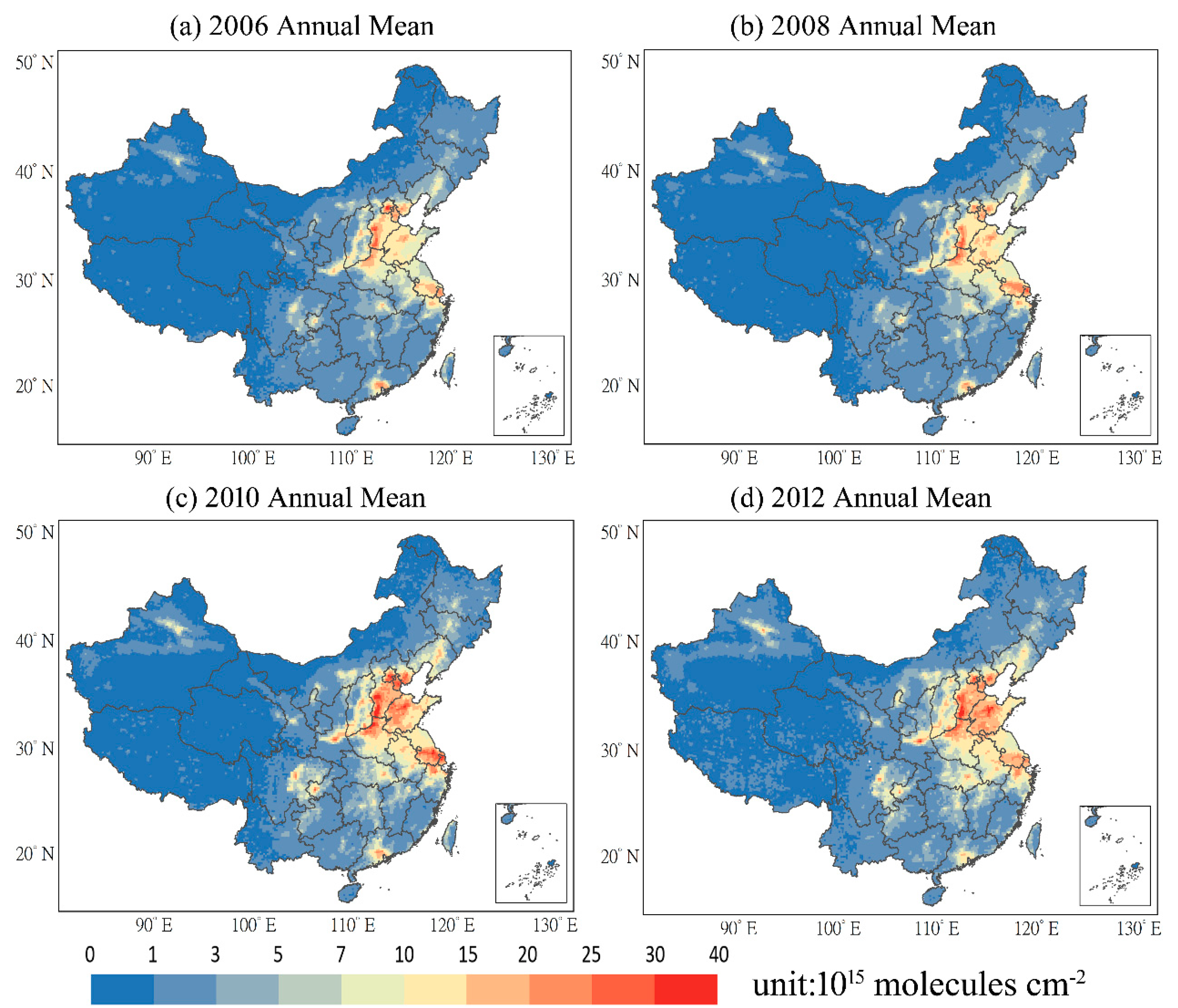
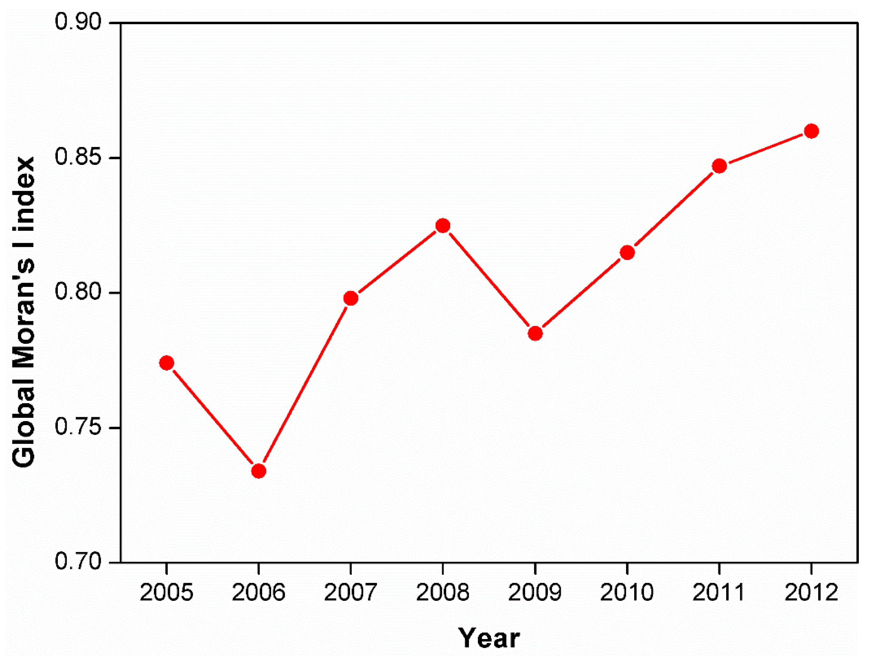
3.1. Spatial Characteristics of NO₂ Pollution over China

Figure 1 shows the spatial distribution of the annual mean tropospheric NO₂ over China in 2006, 2008, 2010, and 2012. The severe NO₂ pollution regions not only covered the traditional urban clustering regions, namely, the North China Plain (NCP, including Beijing, Tianjin, Hebei, Henan and Shandong provinces), the Yangtze River Delta (YRD), and the Pearl River Delta (PRD), but also include Shanxi Province, the Chengyu city-cluster and the Guanzhong city-cluster. As shown in Figure 1, the polluted regions (grids in color from light yellow to red, exceeding 7 × 10¹⁵ molecules cm⁻²) gradually enlarged during this period. Moreover, the NO₂ pollution of most regions presented an increasing trend in these years, particularly the NCP region, Chengyu city-cluster, and Guanzhong city-cluster. On the other hand, the PRD region showed a decreasing trend of NO₂ pollution.

Spatial autocorrelation methods were then employed, including the global Moran’s I method and the hot-spot analysis technique, to further quantify the spatial patterns of tropospheric NO₂ at the city level over China. Euclidean distance and inverse distance conceptualization were chosen for this analysis. Figure 2 shows the results of the application of the global Moran’s I method from 2005 to 2012. Overall, the index exhibited an increasing trend, with two interruptions in 2006 and 2009. The high Moran’s I index values (0.73–0.86) suggest that tropospheric NO₂ exhibited significant clustering over China during this period. We next employed the hot-spot analysis. As shown in Figure 3, the results of the hot-spot analysis at the city level in 2012 revealed that hot-spots are mainly concentrated in the NCP region and the YRD region, while cold-spots are found in the southwest, mainly in Yunnan, Sichuan, Guizhou and Guangxi provinces.

3.2. Regression Model Results

In this subsection, we present and discuss the estimated results of the extended STIRPAT model. However, before addressing these estimations, the Pearson correlation coefficients between variables are reported. These are summarized in

Table 2. Pearson correlation coefficients.

Variable	LnNO2	LnPop	LnPCGDP	LnSTRatio	LnRoad	LnNTL	LnNDVI	LnPres	LnHumi	LnTemp	LnSpeed
LnNO2	1
LnPop	0.6828 [0.0000]	1
LnPCGDP	0.4523 [0.0000]	0.1900 [0.0000]	1
LnSTRatio	0.2308 [0.0000]	0.0432 [0.0567]	0.3087 [0.0000]	1
LnRoad	0.5474 [0.0000]	0.5055 [0.0000]	0.5900 [0.0000]	−0.0776 [0.0006]	1
LnNTL	0.5271 [0.0000]	0.2748 [0.0000]	0.4453 [0.0000]	−0.0344 [0.1290]	0.6473 [0.0000]	1
LnNDVI	−0.0231 [0.3079]	0.3119 [0.0000]	−0.2944 [0.0000]	−0.2389 [0.0000]	−0.0732 [0.0012]	−0.0702 [0.0020]	1
LnPres	−0.0417 [0.0000]	0.4341 [0.0000]	-0.0841 [0.0002]	−0.1443 [0.0000]	0.0449 [0.0476]	−0.1092 [0.0000]	0.7222 [0.0000]	1
LnHumi	−0.1070 [0.0000]	0.4213 [0.0000]	−0.1720 [0.0000]	−0.1487 [0.0000]	−0.0002 [0.9942]	−0.2034 [0.0000]	0.7325 [0.0000]	0.8837 [0.0000]	1
LnTemp	0.1649 [0.0000]	0.5543 [0.0000]	−0.0529 [0.0197]	0.0818 [0.0003]	0.0558 [0.0138]	−0.1430 [0.0000]	0.3881 [0.0000]	0.6836 [0.0000]	0.5866 [0.0000]	1
LnWS	0.2446 [0.0000]	0.0355 [0.1178]	0.3530 [0.0000]	0.0063 [0.7804]	0.2890 [0.0000]	0.4073 [0.0000]	−0.3701 [0.0000]	−0.2689 [0.0000]	−0.3503 [0.0000]	−0.3162 [0.0000]	1

Note: p-values in brackets.

.

We will first present the results of the pooled least squares (PLS) model, since it generally serves as the benchmark model. These results are summarized in

Table 3. Pooled least squares results.

Variable	Coefficient	Std. Err	Probability	VIF	Tolerance
LnPop	0.7449	0.0176	0.0000	2.54	0.3946
LnPCGDP	0.2400	0.0195	0.0000	2.23	0.4476
LnSTRatio	0.1976	0.0248	0.0000	1.43	0.7014
LnRoad	−0.0442	0.0167	0.0080	3.19	0.3130
LnNTL	0.2004	0.0174	0.0000	2.18	0.4589
LnNDVI	0.5498	0.0538	0.0000	3.08	0.3250
LnPres	−0.2134	0.0410	0.0000	7.21	0.1386
LnHumi	−2.1780	0.1679	0.0000	5.80	0.1725
LnTemp	0.0172	0.0332	0.6050	2.97	0.3366
LnWS	−0.0273	0.0477	0.5670	1.60	0.6252
Constant	−8.4091	0.2605	0.0000
R2	0.7514
Adj R2	0.7501
F-Statistic	584.35
p-value (F-Statistic)	0.0000

. As shown in Table 3, all explanatory variables were statistically significant at the 1% significance level. The R² statistic indicates that 75.1% of the total variation of the dependent variable, namely, the NO₂ pollution level, can be explained by these 10 explanatory variables. The results of an F statistic test showed that the null hypothesis of the joint insignificance of all variables can be strongly rejected. In addition, we performed a test for the potential issue of multicollinearity. It was found that the variance inflation factor of each explanatory variable was not greater than 10, indicating that the model did not suffer from the problem. To conclude, the PLS model was well fitted.

Regarding the estimated coefficients, we found that population, per capita GDP, the ratio of the secondary industry to the tertiary industry, total nighttime light data, normalized difference vegetation index, and wind speed were positively correlated with NO₂ pollution, while urban road area, relative humidity, and temperature had negative impacts on NO₂ pollution. We did not expect that the relative humidity would have a negative impact. Moreover, its elasticity coefficient was −2.1780 and may be overestimated. Similarly, the wind speed variable was found to be positive, also contradicting our expectations. The major explanation for these unexpected results was that the PLS model ignored city-specific fixed effects, which may have led to biased results. Hence, we conducted an F test and found that the null hypothesis of the joint insignificance of μ_i could be strongly rejected at the 1% significance level. Hence, we concluded that the fixed effects model may be better fitted than the PLS model. The next step was to compare the results of the fixed effects model and the random effects model. The results are summarized in

Table 4. Results of the fixed effects and random effects models.

	Fixed Effects Model			Random Effects Model
Variable	Coefficient	Std. Err	Probability	Coefficient	Std. Err	Probability
LnPop	0.3874	0.1032	0.0000	0.6855	0.0346	0.0000
LnPCGDP	0.3783	0.0163	0.0000	0.3456	0.0151	0.0000
LnSTRatio	0.1055	0.0377	0.0050	0.1386	0.0325	0.0000
LnRoad	0.0267	0.0135	0.0480	0.0158	0.0131	0.2280
LnNTL	0.0897	0.0233	0.0000	0.1245	0.0202	0.0000
LnNDVI	−0.2064	0.0818	0.0120	−0.1316	0.0648	0.0420
LnPress	0.0439	0.0239	0.0660	0.0240	0.0231	0.2980
LnHumi	−0.6783	0.1272	0.0000	−0.9016	0.1222	0.0000
LnTemp	−0.1592	0.0499	0.0010	−0.2156	0.0399	0.0000
LnSpeed	−0.4169	0.0667	0.0000	−0.3399	0.0581	0.0000
Constant	−5.7434	0.6871	0.0000	−7.5706	0.3597	0.0000
R2	0.5712			0.5655
F-Statistic/Wald Statistic	225.24			2805.35
p-value	0.0000			0.0000

.

We found that all variables in the fixed effects model were statistically significant at least at the 5% significance level. On the contrary, for the random effects model, the variables of NDVI and urban road area were highly insignificant. In order to determine if the fixed effects model was better fitted than the random effects model, we performed a Hausman test. The test results were in favor of the fixed effects model.

The population variable was found to be positive, in line with our expectations, indicating that an increase in population results in NO₂ pollution. The coefficient is 0.3874, indicating that an increase in population of 1% within the dataset was associated with a rise in NO₂ pollution of 0.3874%. Population is mainly attributed to worsening environmental quality, since inhabitants consume a large amount of energy and other resources, and thus generate various pollutants. Although the growth rate of the population of China has been gradually declining during the last decade, more than 1.4 billion people will pose a huge threat to the environment in the long run.

Per capita GDP also had a positive correlation with NO₂ pollution. We found a positive coefficient of 0.3783, meaning that increases in income levels of 1% within the dataset were associated with increases in NO₂ pollution of 0.3783%. We also implemented a robustness check, by testing the quadratic term of the per capita income to verify if this generates an inverted U-shaped curve. Specifically, we assumed that the NO₂ pollution passes a turning point and is then improved as income levels continue to rise. However, we found that the quadratic term was highly insignificant and drew the conclusion that there was an increasingly linear relationship between income and NO₂ pollution.

Regarding the ratio of secondary industry to tertiary industry, it was found that the impact of this ratio on NO₂ pollution was significant and positive, as expected. The positive coefficient, 0.1055, indicated that within the dataset an increase in the share of secondary industry to tertiary industry by 1% was associated with increases in NO₂ pollution of 0.1055%. Secondary industry has long dominated China’s economy, because large-scale industrialization was considered to be the best way to stimulate economic growth and realize common prosperity in the early stage of economic development. As a consequence, secondary industry, the largest pollutant emitter, contributes greatly to the NO₂ pollution in China. Fortunately, China has been experiencing an industrial upgrade in recent years, and the transition from pollution-intensive secondary industry to tertiary industry is characterized by advanced technology and high added value. Hence, it is predicted that industrial upgrades and technological changes will reduce the negative effects on environmental quality.

Nighttime light data, as a proxy for energy consumption, were also found to have a positive relationship with NO₂ pollution, indicating that energy consumption contributes to environmental degradation. Specifically, the positive coefficient, 0.0897, implies that an increase in energy use of 1% within the dataset may lead to increases in NO₂ pollution of 0.0897%. During the past two decades, rapid economic growth in China has consumed a large amount of energy resources, particularly fossil fuels, with coal playing a dominant role in the energy structure. The overuse of fossil fuels generated more NO_x in the air, thus affecting the local environment. The positive coefficient for the total nighttime light data suggests that the government should increase the levels of energy-saving technologies and renewable energy in the energy use structure.

In terms of the urban road area variable, in contrast to the estimated coefficient of the PLS model, it was significant and positive in the fixed effects model, in line with our expectations, implying that the bias had been corrected because the fixed effect has been controlled for in the model. The positive effect of the urban road area (0.0267) on NO₂ pollution indicates that within the dataset an increase in urban road area of 1% caused a rise of NO₂ level of 0.067%.

Vegetation coverage has a negative impact on NO₂ pollution. The negative coefficient, −0.2064, indicates that an increase in the vegetation coverage of 1% within the dataset is associated with a reduction in NO₂ pollution of 0.2064%. The changes in vegetation coverage largely affect local air quality, thus changing the NO₂ concentrations. Therefore, increasing the vegetation coverage can reduce NO₂ concentrations in local city regions.

Meteorological parameters also influence the NO₂ pollution level. We found that cities with a higher temperature, higher relative humidity, higher wind speed, and lower ambient pressure can reduce the NO₂ value.

4. Conclusions and Policy Implications

The main aim of this research is twofold. First, we assessed the spatial and temporal patterns of tropospheric NO₂ columns based on OMI satellite instrument observations. In the second stage, we evaluated the driving factors that influence NO₂ pollution using an extended STIRPAT model. The findings were as follows. The highly NO₂ polluted regions, which are concentrated in certain city-clusters and polluted regions, expanded significantly during 2005–2012. Tropospheric NO₂ exhibited highly clustered spatial patterns over China. We found that those factors that had a positive relationship with tropospheric NO₂ were population, per capita GDP, the share of the secondary industry, ambient air pressure, total nighttime light data, and urban road area, indicating that these influencing factors drive up the NO₂ pollution level. On the other hand, factors that may lower the NO₂ pollution level were NDVI, relative humidity, temperature, and wind speed, which all contributed to reducing the environmental pressure caused by an increase in the NO₂ pollution level. Although the meteorological factors may have a significant influence on the NO₂ pollution level, they cannot be changed directly. Therefore, a transformation of the patterns of human activity is necessary to mitigate NO₂ pollution at the city level in China.

Population and affluence are the major influencing factors driving up the NO₂ pollution level and causing consequent environmental pressures of many kinds. As China’s economy grows and income levels increase, the improvement of living standards has led to increasing demand for energy and resources. The provision of a large number of energy-intensive products and services has also posed a challenge for the environment. Given the fact that China has a large population and is witnessing a rise in income levels, environmental awareness needs to be enhanced. Besides, it is well known that secondary industry is the main contributor to a variety of pollution emissions, and is a major contributing factor to the NO₂ level. We find that it is necessary to focus on industrial upgrades and a rapid transition from highly-polluting secondary industry to tertiary industry, which is characterized by high added value and less pollution. In addition, regarding the highly polluting and largest NO₂-emitting sectors, namely, power plants, steel, and cement, de-nitrification systems that involve selective catalytic or non-catalytic reduction are urgently needed in order to further improve the de-nitrification efficiency and thus reduce the environmental pressure caused by NO₂ emissions from existing sources. With regards to another large source of NO₂ emissions, residential energy use, environmental education should be improved together with the increase in income levels. In order to sustain the trade-off between economic levels and environmental quality, environmental awareness enhancement and low-emission lifestyles should be encouraged.

References

1. Zhang, Q.; Geng, G.; Wang, S.; Richter, A.; He, K.B. Satellite remote sensing of changes in NOx emissions over China during 1996–2010. Chin. Sci. Bull. 2012, 57, 2857–2864. [Google Scholar] [CrossRef]
2. Richter, A.; Burrows, J.P.; Nusz, H.; Granier, C.; Niemeier, U. Increase in tropospheric nitrogen dioxide over China observed from space. Nature 2005, 437, 129–132. [Google Scholar] [CrossRef]
3. WHO. Air Quality Guidelines for Particulate Matter, Ozone, Nitrogen Dioxide and Sulfur Dioxide—Global Update 2005—Summary of Risk Assessmen; WHO: Geneva, Switzerland, 2006. [Google Scholar]
4. He, J.; Gong, S.; Yu, Y.; Yu, L.; Wu, L.; Mao, H.; Song, C.; Zhao, S.; Liu, H.; Li, X.; et al. Air pollution characteristics and their relation to meteorological conditions during 2014–2015 in major Chinese cities. Environ. Pollut. 2017, 223, 484–496. [Google Scholar] [CrossRef] [PubMed]
5. Qin, K.; Rao, L.; Xu, J.; Bai, Y.; Zou, J.; Hao, N.; Li, S.; Yu, C. Estimating Ground Level NO2 Concentrations over Central-Eastern China Using a Satellite-Based Geographically and Temporally Weighted Regression Model. Remote Sens. 2017, 9, 950. [Google Scholar] [CrossRef]
6. Cui, Y.; Lin, J.; Song, C.; Liu, M.; Yan, Y.; Xu, Y.; Huang, B. Rapid growth in nitrogen dioxide pollution over Western China, 2005–2013. Atmos. Chem. Phys. 2016, 16, 6207–6221. [Google Scholar] [CrossRef]
7. Lin, J.T.; Liu, Z.; Zhang, Q.; Liu, H.; Mao, J.; Zhuang, G. Modeling uncertainties for tropospheric nitrogen dioxide columns affecting satellite-based inverse modeling of nitrogen oxides emissions. Atmos. Chem. Phys. 2012, 12, 12255–12275. [Google Scholar] [CrossRef]
8. Zhang, Q.; Streets, D.G.; Carmichael, G.R.; He, K.B.; Huo, H.; Kannari, A.; Klimont, Z.; Park, I.S.; Reddy, S.; Fu, J.S.; et al. Asian emissions in 2006 for the NASA INTEX-B mission. Atmos. Chem. Phys. 2009, 9, 5131–5153. [Google Scholar] [CrossRef]
9. The State Council of the People's Republic of China. The Twelfth Five-Year Plan for Energy Saving and Emission Reduction. 2012. Available online: http://www.gov.cn/zwgk/2012-08/21/content_2207867.htm (accessed on 10 January 2019).
10. MEE. Quantitative Assessment Index of Comprehensive Improvement of Urban Environment in the 12th Five-year Plan and Detailed Rules for its Implementation (In Chinese). 2011. Available online: http://www.mee.gov.cn/gkml/hbb/bgth/201111/t20111116_220023.htm (accessed on 2 January 2019).
11. van der A, R.J.; Peters, D.H.M.U.; Eskes, H.; Boersma, K.F.; Van Roozendael, M.; De Smedt, I.; Kelder, H.M. Detection of the trend and seasonal variation in tropospheric NO2 over China. J. Geo Res. Atmos. 2006, 111, D12317. [Google Scholar] [CrossRef]
12. Gu, D.; Wang, Y.; Smeltzer, C.; Liu, Z. Reduction in NOx Emission Trends over China: Regional and Seasonal Variations. Environ. Sci. Technol. 2013, 47, 12912–12919. [Google Scholar] [CrossRef]
13. Streets, D.G.; Canty, T.; Carmichael, G.R.; de Foy, B.; Dickerson, R.R.; Duncan, B.N.; Edwards, D.P.; Haynes, J.A.; Henze, D.K.; Houyoux, M.R.; et al. Emissions estimation from satellite retrievals: A review of current capability. Atmos. Environ. 2013, 77, 1011–1042. [Google Scholar] [CrossRef]
14. Lamsal, L.N.; Krotkov, N.A.; Celarier, E.A.; Swartz, W.H.; Pickering, K.E.; Bucsela, E.J.; Gleason, J.F.; Martin, R.V.; Philip, S.; Irie, H.; et al. Evaluation of OMI operational standard NO2 column retrievals using in situ and surface-based NO2 observations. Atmos. Chem. Phys. 2014, 14, 11587–11609. [Google Scholar] [CrossRef]
15. de Foy, B.; Lu, Z.; Streets, D.G. Satellite NO2 retrievals suggest China has exceeded its NOx reduction goals from the twelfth Five-Year Plan. Sci. Rep. 2016, 6, 35912. [Google Scholar] [CrossRef]
16. Zhao, J.; Chen, S.; Wang, H.; Ren, Y.; Du, K.; Xu, W.; Zheng, H.; Jiang, B. Quantifying the impacts of socio-economic factors on air quality in Chinese cities from 2000 to 2009. Environ. Pollut. 2012, 167, 148–154. [Google Scholar] [CrossRef] [PubMed]
17. Lyu, W.; Li, Y.; Guan, D.; Zhao, H.; Zhang, Q.; Liu, Z. Driving forces of Chinese primary air pollution emissions: an index decomposition analysis. J. Clean. Prod. 2016, 133, 136–144. [Google Scholar] [CrossRef]
18. Zhang, J.; Ouyang, Z.; Miao, H.; Wang, X. Ambient air quality trends and driving factor analysis in Beijing, 1983–2007. J. Environ. Sci. 2011, 23, 2019–2028. [Google Scholar] [CrossRef]
19. Lin, X.; Wang, D. Spatiotemporal evolution of urban air quality and socioeconomic driving forces in China. J. Geograph. Sci. 2016, 26, 1533–1549. [Google Scholar] [CrossRef]
20. Du, Y.; Sun, T.; Peng, J.; Fang, K.; Liu, Y.; Yang, Y.; Wang, Y. Direct and spillover effects of urbanization on PM2.5 concentrations in China's top three urban agglomerations. J. Clean. Prod. 2018, 190, 72–83. [Google Scholar] [CrossRef]
21. Jiang, L.; Zhou, H.-f.; Bai, L.; Zhou, P. Does foreign direct investment drive environmental degradation in China? An empirical study based on air quality index from a spatial perspective. J. Clean. Prod. 2018, 176, 864–872. [Google Scholar] [CrossRef]
22. Liu, H.; Fang, C.; Zhang, X.; Wang, Z.; Bao, C.; Li, F. The effect of natural and anthropogenic factors on haze pollution in Chinese cities: A spatial econometrics approach. J. Clean. Prod. 2017, 165, 323–333. [Google Scholar] [CrossRef]
23. Huang, J.; Zhou, C.; Lee, X.; Bao, Y.; Zhao, X.; Fung, J.; Richter, A.; Liu, X.; Zheng, Y. The effects of rapid urbanization on the levels in tropospheric nitrogen dioxide and ozone over East China. Atmos. Environ. 2013, 77, 558–567. [Google Scholar] [CrossRef]
24. Lee, H.J.; Koutrakis, P. Daily ambient NO2 concentration predictions using satellite ozone monitoring instrument NO2 data and land use regression. Environ. Sci. Technol. 2014, 48, 2305–2311. [Google Scholar]
25. Xiao, H.; Ma, Z.; Mi, Z.; Kelsey, J.; Zheng, J.; Yin, W.; Yan, M. Spatio-temporal simulation of energy consumption in China's provinces based on satellite night-time light data. Appl. Energy 2018, 231, 1070–1078. [Google Scholar] [CrossRef]
26. Letu, H.; Hara, M.; Yagi, H.; Naoki, K.; Tana, G.; Nishio, F.; Shuhei, O. Estimating energy consumption from night-time DMPS/OLS imagery after correcting for saturation effects. Int. J. Remote Sens. 2010, 31, 4443–4458. [Google Scholar] [CrossRef]
27. Amaral, S.; Câmara, G.; Monteiro, A.M.V.; Quintanilha, J.A.; Elvidge, C.D. Estimating population and energy consumption in Brazilian Amazonia using DMSP night-time satellite data. Comp. Environ. Urban Syst. 2005, 29, 179–195. [Google Scholar] [CrossRef]
28. Martínez, B.; Gilabert, M.A. Vegetation dynamics from NDVI time series analysis using the wavelet transform. Remote Sens. Environ. 2009, 113, 1823–1842. [Google Scholar] [CrossRef]
29. Tobler, W.R. Cellular Geography. In Philosophy in Geography; Gale, S., Olsson, G., Eds.; Springer: Dordrecht, The Netherlands, 1979; pp. 379–386. [Google Scholar]
30. Dong, L.; Liang, H. Spatial analysis on China's regional air pollutants and CO2 emissions: emission pattern and regional disparity. Atmos. Environ. 2014, 92, 280–291. [Google Scholar] [CrossRef]
31. Ehrlich, P.R.; Holdren, J.P. Impact of population growth. Science 1971, 171, 1212–1217. [Google Scholar] [CrossRef]
32. Li, H.; Mu, H.; Zhang, M.; Li, N. Analysis on influence factors of China's CO2 emissions based on Path–STIRPAT model. Energy Policy 2011, 39, 6906–6911. [Google Scholar] [CrossRef]
33. Wang, P.; Wu, W.; Zhu, B.; Wei, Y. Examining the impact factors of energy-related CO2 emissions using the STIRPAT model in Guangdong Province, China. Appl. Energy 2013, 106, 65–71. [Google Scholar] [CrossRef]
34. Xu, B.; Lin, B. Assessing CO2 emissions in China's iron and steel industry: a nonparametric additive regression approach. Renew. Sustain. Energy Rev. 2017, 72, 325–337. [Google Scholar] [CrossRef]
35. Wang, Y.; Han, R.; Kubota, J. Is there an environmental Kuznets curve for SO2 emissions? A semi-parametric panel data analysis for China. Renew. Sustain. Energy Rev. 2016, 54, 1182–1188. [Google Scholar] [CrossRef]
36. Yang, X.; Wang, S.; Zhang, W.; Li, J.; Zou, Y. Impacts of energy consumption, energy structure, and treatment technology on SO2 emissions: A multi-scale LMDI decomposition analysis in China. Appl Energy 2016, 184, 714–726. [Google Scholar] [CrossRef]
37. Shahbaz, M.; Loganathan, N.; Sbia, R.; Afza, T. The effect of urbanization, affluence and trade openness on energy consumption: A time series analysis in Malaysia. Renew. Sustain. Energy Rev. 2015, 47, 683–693. [Google Scholar] [CrossRef]
38. Yang, Y.; Liu, J.; Zhang, Y. An analysis of the implications of China’s urbanization policy for economic growth and energy consumption. J. Clean. Product. 2017, 161, 1251–1262. [Google Scholar] [CrossRef]
39. Liu, Y.; Zhou, Y.; Wu, W. Assessing the impact of population, income and technology on energy consumption and industrial pollutant emissions in China. Appl. Energy 2015, 155, 904–917. [Google Scholar] [CrossRef]
40. Ren, S.; Li, X.; Yuan, B.; Li, D.; Chen, X. The effects of three types of environmental regulation on eco-efficiency: A cross-region analysis in China. J. Clean. Product. 2018, 173, 245–255. [Google Scholar] [CrossRef]
41. Dietz, T.; Rosa, E.A. Effects of population and affluence on CO2 emissions. Proc. Natl. Acad. Sci. USA 1997, 94, 175–179. [Google Scholar] [CrossRef]
42. Li, R.; Leung, G.C.K. Coal consumption and economic growth in China. Energy Policy 2012, 40, 438–443. [Google Scholar] [CrossRef]
43. Doll, C.N.H.; Muller, J.-P.; Morley, J.G. Mapping regional economic activity from night-time light satellite imagery. Ecol. Econ. 2006, 57, 75–92. [Google Scholar] [CrossRef]
44. Ma, T.; Zhou, C.; Pei, T.; Haynie, S.; Fan, J. Quantitative estimation of urbanization dynamics using time series of DMSP/OLS nighttime light data: A comparative case study from China's cities. Remote Sens. Environ. 2012, 124, 99–107. [Google Scholar] [CrossRef]
45. Cui, Y.; Zhang, W.; Bao, H.; Wang, C.; Cai, W.; Yu, J.; Streets, D.G. Spatiotemporal dynamics of nitrogen dioxide pollution and urban development: Satellite observations over China, 2005–2016. Resour. Conserv. Recycl. 2019, 142, 59–68. [Google Scholar] [CrossRef]
46. Meng, L.; Graus, W.; Worrell, E.; Huang, B. Estimating CO2 (carbon dioxide) emissions at urban scales by DMSP/OLS (Defense Meteorological Satellite Program's Operational Linescan System) nighttime light imagery: Methodological challenges and a case study for China. Energy 2014, 71, 468–478. [Google Scholar] [CrossRef]
47. Liu, F.; Zhang, Q.; van der A, R.J.; Zheng, B.; Tong, D.; Yan, L.; Zheng, B.; He, K. Recent reduction in NOx emissions over China: synthesis of satellite observations and emission inventories. Environ. Res. Lett. 2016, 11, 114002. [Google Scholar] [CrossRef]
48. Boersma, K.F.; Eskes, H.J.; Dirksen, R.J.; van der A, R.J.; Veefkind, J.P.; Stammes, P.; Huijnen, V.; Kleipool, Q.L.; Sneep, M.; Claas, J.; et al. An improved tropospheric NO2 column retrieval algorithm for the Ozone Monitoring Instrument. Atmos. Meas. Tech. 2011, 4, 1905–1928. [Google Scholar] [CrossRef]
49. Zhang, Q.; Pandey, B.; Seto, K.C. A Robust Method to Generate a Consistent Time Series From DMSP/OLS Nighttime Light Data. IEEE Trans. Geosci. Remote Sens. 2016, 54, 5821–5831. [Google Scholar] [CrossRef]
50. Bartlett, D.S.; Whiting, G.J.; Hartman, J.M. Use of vegetation indices to estimate indices to estimate intercepted solar radiation and net carbon dioxide exchange of a grass canopy. Remote Sens. Environ. 1989, 30, 115–128. [Google Scholar] [CrossRef]
51. NBS. China Statistical Yearbook 2005-2012, Chinese-English ed.; China Statistics Press: Beijing, China, 2006–2013. [Google Scholar]
52. CCS. China City Statistical Yearbook 2005–2012, Chinese-English ed.; China Statistics Press: Beijing, China, 2006–2013. [Google Scholar]
Figure 1. Spatial distribution of annual mean tropospheric NO2 over China in 2006, 2008, 2010 and 2012.
Ijerph 16 01487 g001
Figure 2. Global Moran’s I values at the city level from 2005 to 2012.
Ijerph 16 01487 g002
Figure 3. Hot-spot analysis over China in 2012.
Ijerph 16 01487 g003