Diurnal and Seasonal Variations in the Effect of Urban Environmental Factors on Air Temperature: A Consecutive Regression Analysis Approach


Abstract
:1. Introduction
2. Literature Review: Effect of Urban Factors on Temperature
3. Methods
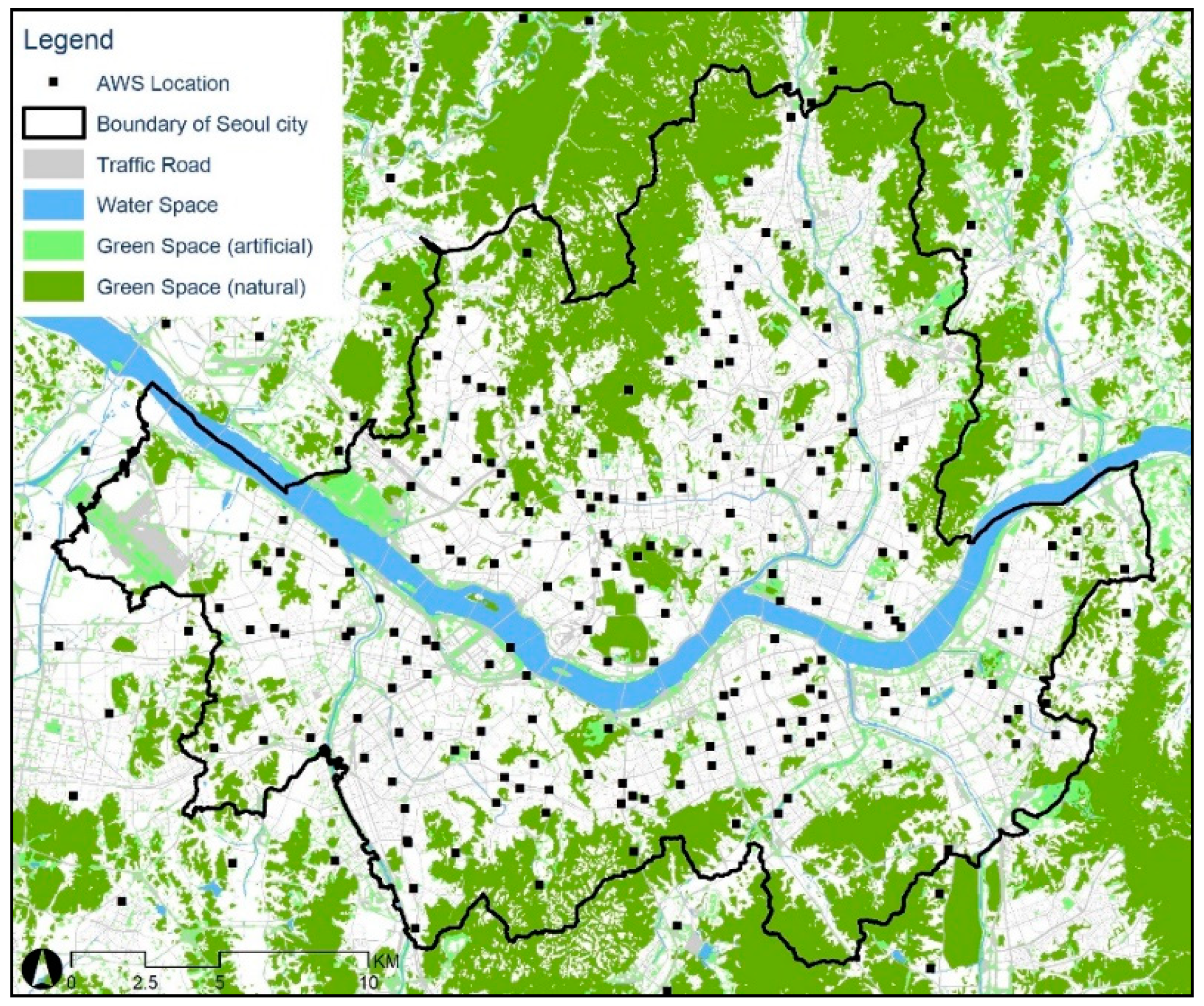
3.1. Study Area
3.2. Dependent Variable
3.3. Independent Variables
3.4. Methodology
4. Results
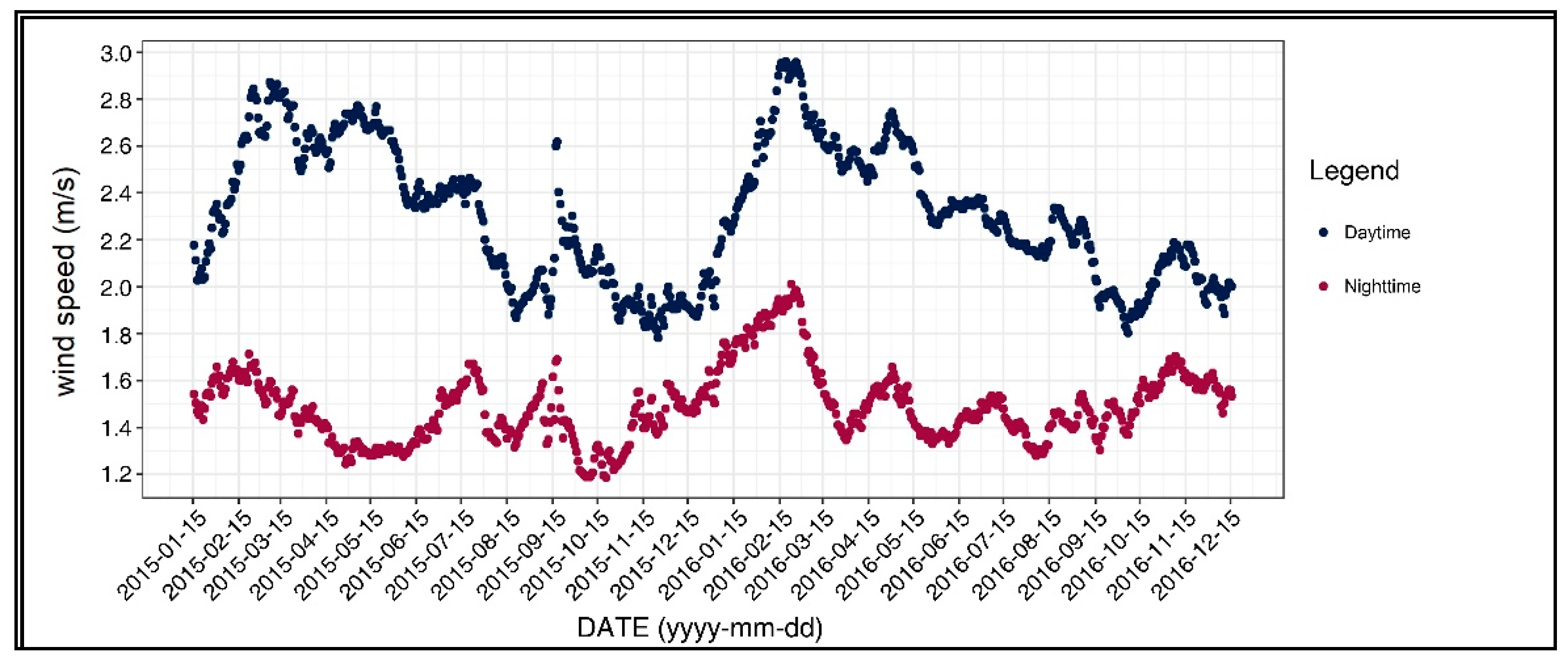
4.1. Descriptive Analysis
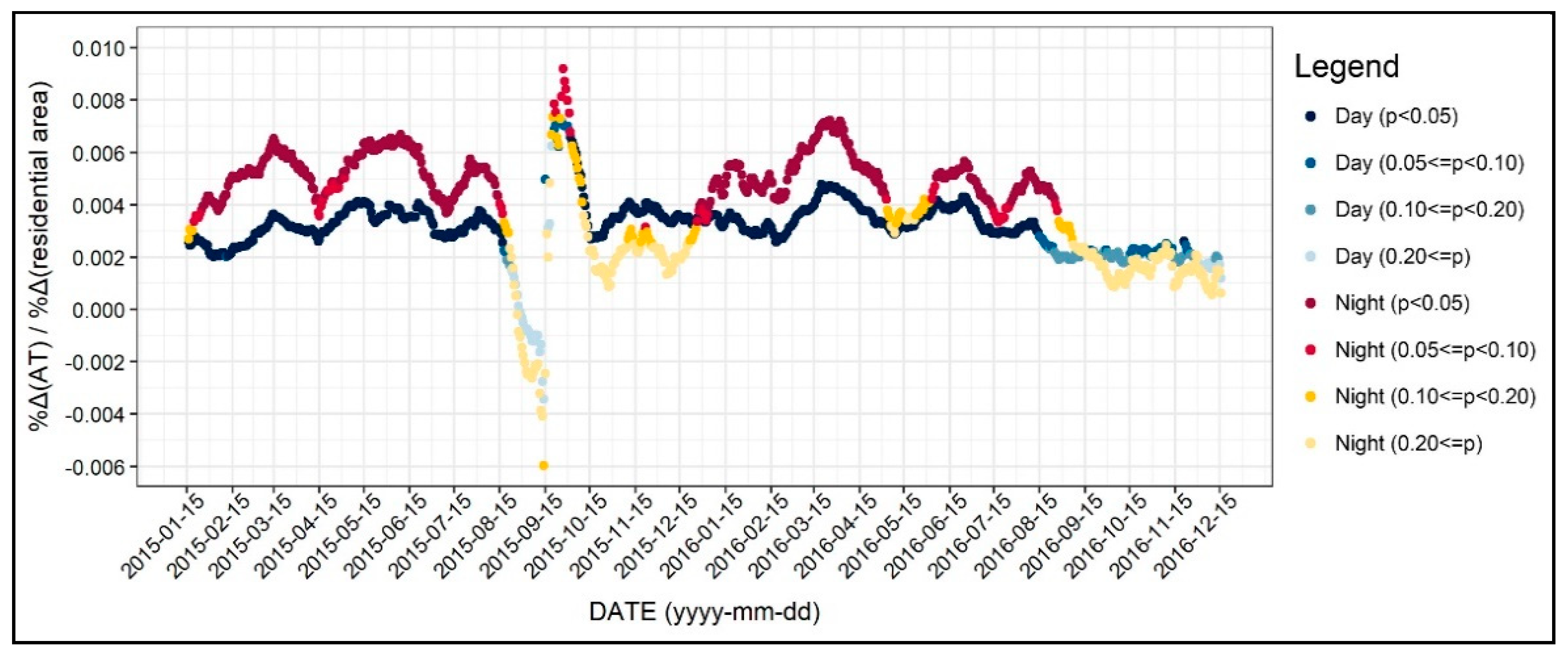
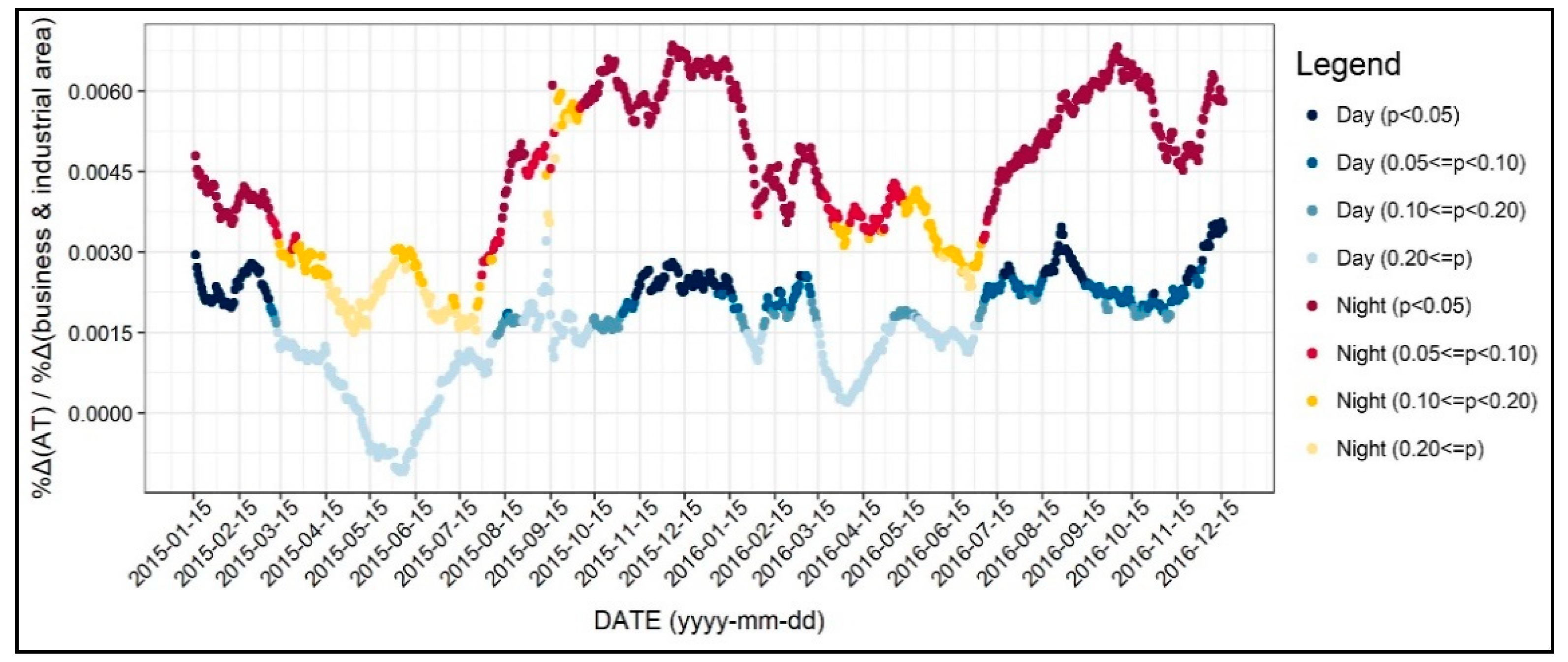
4.2. Consecutive Regression Analysis
5. Discussion
6. Conclusions
Author Contributions
Funding
Conflicts of Interest
References
- Oke, T. Boundary Layer Climates; Routledge: London, UK, 1988. [Google Scholar]
- Oke, T. The energetic basis of the urban heat island. Q. J. R. Meteorol. Soc. 1982, 108, 1–24. [Google Scholar] [CrossRef]
- Solecki, W.D.; Rosenzweig, C.; Parshall, L.; Pope, G.; Clark, M.; Cox, J.; Wiencke, M. Mitigation of the heat island effect in urban New Jersey. Glob. Environ. Chang. Part B Environ. Hazards 2005, 6, 39–49. [Google Scholar] [CrossRef]
- Kim, Y.H.; Baik, J.J. Spatial and temporal structure of the urban heat island in Seoul. J. Appl. Meteorol. 2005, 44, 591–605. [Google Scholar] [CrossRef]
- Kovats, R.S.; Hajat, S. Heat stress and public health: A critical review. Annu. Rev. Public Health 2007, 29, 41–55. [Google Scholar] [CrossRef]
- Santamouris, M. Using cool pavements as a mitigation strategy to fight urban heat island—A review of the actual developments. Renew. Sustain. Energy Rev. 2013, 26, 224–240. [Google Scholar] [CrossRef]
- Wang, Y.; Akbari, H. Analysis of urban heat island phenomenon and mitigation solutions evaluation for Montreal. Sustain. Cities Soc. 2016, 26, 438–446. [Google Scholar] [CrossRef]
- Naserikia, M.; Asadi Shamsabadi, E.; Rafieian, M.; Leal Filho, W. The urban heat island in an urban context: A case study of Mashhad, Iran. Int. J. Environ. Res. Public Health 2019, 16, 313. [Google Scholar] [CrossRef] [Green Version]
- Nunez, M.; Oke, T.R. The energy balance of an urban canyon. J. Appl. Meteorol. 1977, 16, 11–19. [Google Scholar] [CrossRef]
- Oke, T. Canyon geometry and the urban heat island. J. Climatol. 1981, 1, 237–254. [Google Scholar] [CrossRef]
- Chun, B.; Guhathakurta, S. Daytime and nighttime urban heat islands statistical models for Atlanta. Environ. Plan. B Urban Anal. City Sci. 2017, 44, 308–327. [Google Scholar] [CrossRef]
- Gál, T.; Unger, J. Detection of ventilation paths using high-resolution roughness parameter mapping in a large urban area. Build. Environ. 2009, 44, 198–206. [Google Scholar] [CrossRef]
- Park, C.; Ha, J.; Lee, S. Association between three-dimensional built environment and urban air temperature: Seasonal and temporal differences. Sustainability 2017, 9, 1338. [Google Scholar] [CrossRef] [Green Version]
- Bottyán, Z.; Unger, J. A multiple linear statistical model for estimating the mean maximum urban heat island. Theor. Appl. Climatol. 2003, 75, 233–243. [Google Scholar] [CrossRef]
- Eliasson, I. Urban nocturnal geometry temperatures, and land use. Atmos. Environ. 1996, 30, 379–392. [Google Scholar] [CrossRef]
- Yokobori, T.; Ohta, S. Effect of land cover on air temperatures involved in the development of an intra-urban heat island. Clim. Res. 2009, 39, 61–73. [Google Scholar] [CrossRef]
- Chun, B.; Guldmann, J.M. Impact of greening on the urban heat island: Seasonal variations and mitigation strategies. Comput. Environ. Urban Syst. 2018, 71, 165–176. [Google Scholar] [CrossRef]
- Yan, H.; Fan, S.; Guo, C.; Wu, F.; Zhang, N.; Dong, L. Assessing the effects of landscape design parameters on intra-urban air temperature variability: The case of Beijing, China. Build. Environ. 2014, 76, 44–53. [Google Scholar] [CrossRef]
- Gál, T.; Lindberg, F.; Unger, J. Computing continuous sky view factors using 3D urban raster and vector databases: Comparison and application to urban climate. Theor. Appl. Climatol. 2009, 95, 111–123. [Google Scholar] [CrossRef]
- Chun, B.; Guhathakurta, S. The impacts of three-dimensional surface characteristics on urban heat islands over the diurnal cycle. Prof. Geogr. 2017, 69, 191–202. [Google Scholar] [CrossRef]
- Shiflett, S.A.; Liang, L.L.; Crum, S.M.; Feyisa, G.L.; Wang, J.; Jenerette, G.D. Variation in the urban vegetation, surface temperature, air temperature nexus. Sci. Total Environ. 2017, 579, 495–505. [Google Scholar] [CrossRef]
- Wang, Y.; Berardi, U.; Akbari, H. Comparing the effects of urban heat island mitigation strategies for Toronto, Canada. Energy Build. 2016, 114, 2–19. [Google Scholar] [CrossRef]
- Taha, H. Urban climates and heat islands: Albedo, evapotranspiration, and anthropogenic heat. Energy Build. 1997, 25, 99–103. [Google Scholar] [CrossRef] [Green Version]
- Giridharan, R.; Lau, S.S.Y.; Ganesan, S. Nocturnal heat island effect in urban residential developments of Hong Kong. Energy Build. 2005, 37, 964–971. [Google Scholar] [CrossRef]
- Klok, L.; Zwart, S.; Verhagen, H.; Mauri, E. The surface heat island of Rotterdam and its relationship with urban surface characteristics. Resour. Conserv. Recycl. 2012, 64, 23–29. [Google Scholar] [CrossRef]
- Liu, W.; Feddema, J.; Hu, L.; Zung, A.; Brunsell, N. Seasonal and diurnal characteristics of land surface temperature and major explanatory factors in Harris County, Texas. Sustainability 2017, 9, 2324. [Google Scholar] [CrossRef] [Green Version]
- Yang, J.; Wang, Z.H.; Kaloush, K.E. Environmental impacts of reflective materials: Is high albedo a “silver bullet” for mitigating urban heat island? Renew. Sustain. Energy Rev. 2015, 47, 830–843. [Google Scholar] [CrossRef] [Green Version]
- Hamada, S.; Ohta, T. Seasonal variations in the cooling effect of urban green areas on surrounding urban areas. Urban For. Urban Green. 2010, 9, 15–24. [Google Scholar] [CrossRef]
- Jusuf, S.K.; Wong, N.H.; Hagen, E.; Anggoro, R.; Hong, Y. The influence of land use on the urban heat island in Singapore. Habitat Int. 2007, 31, 232–242. [Google Scholar] [CrossRef]
- Bokaie, M.; Shamsipour, A.; Khatibi, P.; Hosseini, A. Seasonal monitoring of urban heat island using multi-temporal Landsat and MODIS images in Tehran. Int. J. Urban Sci. 2019, 23, 269–285. [Google Scholar] [CrossRef]
- Van, T.T.; Bao, H.D.X. Study of the impact of urban development on surface temperature using remote sensing in Ho Chi Minh City, Northern Vietnam. Geogr. Res. 2010, 48, 86–96. [Google Scholar] [CrossRef]
- Hart, M.A.; Sailor, D.J. Quantifying the influence of land-use and surface characteristics on spatial variability in the urban heat island. Theor. Appl. Climatol. 2009, 95, 397–406. [Google Scholar] [CrossRef]
- Zhang, G.; He, B.J.; Zhu, Z.; Dewancker, B.J. Impact of morphological characteristics of green roofs on pedestrian cooling in subtropical climates. Int. J. Environ. Res. Public Health 2019, 16, 179. [Google Scholar] [CrossRef] [PubMed] [Green Version]
- Krüger, E.; Givoni, B. Outdoor measurements and temperature comparisons of seven monitoring stations: Preliminary studies in Curitiba, Brazil. Build. Environ. 2007, 42, 1685–1698. [Google Scholar] [CrossRef]
- Morabito, M.; Crisci, A.; Messeri, A.; Orlandini, S.; Raschi, A.; Maracchi, G.; Munafò, M. The impact of built-up surfaces on land surface temperatures in Italian urban areas. Sci. Total Environ. 2016, 551–552, 317–326. [Google Scholar] [CrossRef]
- Kim, H.; Kim, S.N. The seasonal and diurnal influence of surrounding land use on temperature: Findings from Seoul, South Korea. Sustainability 2017, 9, 1443. [Google Scholar] [CrossRef] [Green Version]
- Bowler, D.E.; Buyung-Ali, L.; Knight, T.M.; Pullin, A.S. Urban greening to cool towns and cities: A systematic review of the empirical evidence. Landsc. Urban Plan. 2010, 97, 147–155. [Google Scholar] [CrossRef]
- Shashua-Bar, L.; Hoffman, M.E. Vegetation as a climatic component in the design of an urban street. Energy Build. 2002, 31, 221–235. [Google Scholar] [CrossRef]
- Cai, Z.; Han, G.; Chen, M. Do water bodies play an important role in the relationship between urban form and land surface temperature? Sustain. Cities Soc. 2018, 39, 487–498. [Google Scholar] [CrossRef]
- Dai, Z.; Guldmann, J.M.; Hu, Y. Spatial regression models of park and land-use impacts on the urban heat island in central Beijing. Sci. Total Environ. 2018, 626, 1136–1147. [Google Scholar] [CrossRef]
- Zhang, Y.; Murray, A.T.; Turner, B.L. Optimizing green space locations to reduce daytime and nighttime urban heat island effects in Phoenix, Arizona. Landsc. Urban Plan. 2017, 165, 162–171. [Google Scholar] [CrossRef]
- Chow, W.T.L.; Roth, M. Temporal dynamics of the urban heat island of Singapore. Int. J. Climatol. 2006, 26, 2243–2260. [Google Scholar] [CrossRef]
- Lan, Y.; Zhan, Q. How do urban buildings impact summer air temperature? The effects of building configurations in space and time. Build. Environ. 2017, 125, 88–98. [Google Scholar] [CrossRef]
- Yue, W.; Liu, X.; Zhou, Y.; Liu, Y. Impacts of urban configuration on urban heat island: An empirical study in China mega-cities. Sci. Total Environ. 2019, 671, 1036–1046. [Google Scholar] [CrossRef]
- Yuan, C.; Chen, L. Mitigating urban heat island effects in high-density cities based on sky view factor and urban morphological understanding: A study of Hong Kong. Archit. Sci. Rev. 2011, 54, 305–315. [Google Scholar] [CrossRef]
- Yang, F.; Lau, S.S.Y.; Qian, F. Urban design to lower summertime outdoor temperatures: An empirical study on high-rise housing in Shanghai. Build. Environ. 2011, 46, 769–785. [Google Scholar] [CrossRef]
- Yin, C.; Yuan, M.; Lu, Y.; Huang, Y.; Liu, Y. Effects of urban form on the urban heat island effect based on spatial regression model. Sci. Total Environ. 2018, 634, 696–704. [Google Scholar] [CrossRef] [PubMed]
- Bourbia, F.; Boucheriba, F. Impact of street design on urban microclimate for semi arid climate (Constantine). Renew. Energy 2010, 35, 343–347. [Google Scholar] [CrossRef]
- Eliasson, I.; Svensson, M.K. Spatial air temperature variations and urban land use—A statistical approach. Meteorol. Appl. 2003, 10, 135–149. [Google Scholar] [CrossRef]
- Chen, L.; Ng, E.; An, X.; Ren, C.; Lee, M.; Wang, U.; He, Z. Sky view factor analysis of street canyons and its implications for daytime intra-urban air temperature differentials in high-rise, high-density urban areas of Hong Kong: A GIS-based simulation approach. Int. J. Climatol. 2012, 32, 121–136. [Google Scholar] [CrossRef]
- Gong, F.Y.; Zeng, Z.C.; Zhang, F.; Li, X.; Ng, E.; Norford, L.K. Mapping sky, tree, and building view factors of street canyons in a high-density urban environment. Build. Environ. 2018, 134, 155–167. [Google Scholar] [CrossRef]
- Unger, J. Intra-urban relationship between surface geometry and urban heat island: Review and new approach. Clim. Res. 2004, 27, 253–264. [Google Scholar] [CrossRef] [Green Version]
- Ayanlade, A. Seasonality in the daytime and night-time intensity of land surface temperature in a tropical city area. Sci. Total Environ. 2016, 557–558, 415–424. [Google Scholar] [CrossRef] [PubMed]
- Yao, R.; Wang, L.; Huang, X.; Niu, Z.; Liu, F.; Wang, Q. Temporal trends of surface urban heat islands and associated determinants in major Chinese cities. Sci. Total Environ. 2017, 609, 742–754. [Google Scholar] [CrossRef] [PubMed]
- Quan, J. Multi-temporal effects of urban forms and functions on urban heat islands based on local climate zone classification. Int. J. Environ. Res. Public Health 2019, 16, 2140. [Google Scholar] [CrossRef] [Green Version]
- Tong, S.; Wong, N.H.; Jusuf, S.K.; Tan, C.L.; Wong, H.F.; Ignatius, M.; Tan, E. Study on correlation between air temperature and urban morphology parameters in built environment in northern China. Build. Environ. 2018, 127, 239–249. [Google Scholar] [CrossRef]
- Korea Meteorological Administration. Climate Change Forecast Report of Korean Peninsula; Number of Report 11-1360000-000861-01; Korea Meteorological Administration: Seoul, Korea, 2012.
- Lee, S.H.; Baik, J.J. Statistical and dynamical characteristics of the urban heat island intensity in Seoul. Theor. Appl. Climatol. 2010, 100, 227–237. [Google Scholar] [CrossRef]
- Kim, Y.; Choi, Y. A study on the intensity of urban heat islands in the Seoul metropolitan area by weather condition. Geogr. J. Korea 2012, 46, 1–9. [Google Scholar]
- Peel, M.C.; Finlayson, B.L.; McMahon, T.A. Updated world map of the Köppen-Geiger climate classification. Hydrol. Earth Syst. Sci. 2007, 11, 1633–1644. [Google Scholar] [CrossRef] [Green Version]
- Oke, T. World meteorological organization instruments and observing methods. In Initial Guidance to Obtain Representative Meteorological Observations at Urban Sites; World Meteorological Organization: Geneva, Switzerland, 2004. [Google Scholar]
- Schrijvers, P.J.C.; Jonker, H.J.J.; De Roode, S.R.; Kenjereš, S. The effect of using a high-albedo material on the Universal Temperature Climate Index within a street canyon. Urban Clim. 2016, 17, 284–303. [Google Scholar] [CrossRef]
- Hoffmann, P.; Fischereit, J.; Heitmann, S.; Schlünzen, K.H.; Gasser, I. Modeling exposure to heat stress with a simple urban model. Urban Sci. 2018, 2, 9. [Google Scholar] [CrossRef] [Green Version]
- Coseo, P.; Larsen, L. How factors of land use/land cover, building configuration, and adjacent heat sources and sinks explain Urban Heat Islands in Chicago. Landsc. Urban Plan. 2014, 125, 117–129. [Google Scholar] [CrossRef]


| Variable | Unit | Mean | St. Dev * | Min. | Max. | VIF ** |
|---|---|---|---|---|---|---|
| AWS altitude [ALT] | m | 63.136 | 33.001 | 9.727 | 332.600 | 1.56 |
| Surface albedo [SA] | - | 0.100 | 0.007 | 0.078 | 0.129 | 3.26 |
| Residential use (floor area) [RA] | km2 | 0.585 | 0.347 | 0.000 | 1.489 | 3.81 |
| Commercial use (floor area) [CA] | km2 | 0.107 | 0.106 | 0.000 | 0.637 | 2.36 |
| Busi. & Industrial use (floor area) [BA] | km2 | 0.202 | 0.300 | 0.000 | 2.163 | 2.28 |
| Traffic road area [TA] | km2 | 0.119 | 0.060 | 0.000 | 0.593 | 2.23 |
| Building floor average [BF] | - | 3.866 | 2.004 | 1.043 | 19.851 | 1.81 |
| Area sky view factor [SVF] | - | 0.630 | 0.124 | 0.368 | 0.999 | 4.47 |
| Artificial green area [AG] | km2 | 0.049 | 0.051 | 0.000 | 0.350 | 1.74 |
| Natural green area [NG] | km2 | 0.088 | 0.133 | 0.000 | 0.689 | 4.23 |
| Water area [WA] | km2 | 0.013 | 0.042 | 0.000 | 0.406 | 3.02 |
| Variable | ALT | SA | RA | CA | BA | TA | BF | SVF | AG | NG | WA |
|---|---|---|---|---|---|---|---|---|---|---|---|
| ALT | 1.000 | ||||||||||
| SA | −0.010 | 1.000 | |||||||||
| RA | −0.171 | −0.475 | 1.000 | ||||||||
| CA | −0.093 | −0.288 | 0.090 | 1.000 | |||||||
| BA | −0.017 | −0.254 | −0.018 | 0.664 | 1.000 | ||||||
| TA | −0.291 | −0.183 | 0.168 | 0.477 | 0.388 | 1.000 | |||||
| BF | −0.121 | −0.168 | 0.415 | 0.190 | 0.229 | 0.405 | 1.000 | ||||
| SVF | 0.159 | 0.479 | −0.609 | −0.354 | −0.211 | −0.070 | 0.120 | 1.000 | |||
| AG | −0.093 | 0.270 | −0.230 | −0.253 | −0.182 | 0.114 | 0.209 | 0.550 | 1.000 | ||
| NG | 0.526 | 0.246 | −0.534 | −0.410 | −0.310 | −0.570 | −0.256 | 0.521 | 0.037 | 1.000 | |
| WA | −0.216 | −0.224 | −0.176 | −0.147 | −0.122 | 0.100 | 0.158 | 0.396 | 0.325 | −0.087 | 1.000 |
© 2020 by the authors. Licensee MDPI, Basel, Switzerland. This article is an open access article distributed under the terms and conditions of the Creative Commons Attribution (CC BY) license (http://creativecommons.org/licenses/by/4.0/).
Share and Cite
Ha, J.; Choi, Y.; Lee, S.; Oh, K. Diurnal and Seasonal Variations in the Effect of Urban Environmental Factors on Air Temperature: A Consecutive Regression Analysis Approach. Int. J. Environ. Res. Public Health 2020, 17, 421. https://doi.org/10.3390/ijerph17020421
Ha J, Choi Y, Lee S, Oh K. Diurnal and Seasonal Variations in the Effect of Urban Environmental Factors on Air Temperature: A Consecutive Regression Analysis Approach. International Journal of Environmental Research and Public Health. 2020; 17(2):421. https://doi.org/10.3390/ijerph17020421
Chicago/Turabian StyleHa, Jaehyun, Yeri Choi, Sugie Lee, and Kyushik Oh. 2020. "Diurnal and Seasonal Variations in the Effect of Urban Environmental Factors on Air Temperature: A Consecutive Regression Analysis Approach" International Journal of Environmental Research and Public Health 17, no. 2: 421. https://doi.org/10.3390/ijerph17020421