Article

Some Observational and Modeling Studies of the Atmospheric Boundary Layer at Mississippi Gulf Coast for Air Pollution Dispersion Assessment

by
Anjaneyulu Yerramilli
1,*,
Venkata Srinivas Challa
1,
Jayakumar Indracanti
1,
Hariprasad Dasari
1,
Julius Baham
1,
Chuck Patrick
1,
John Young
1,
Robert Hughes
1,
Lorren D. White
2,
Mark G. Hardy
1 and
Shelton Swanier
1
1
Trent Lott Geospatial and Visualization Research Centre, @e-Centre, Raymond Road, College of Science Engineering & Technology (CSET), Jackson State University, Mississippi 39217, USA
2
Department of Physics, Atmospheric Sciences and Geo Sciences, CSET, JSU, Jackson, Mississippi, USA
*
Author to whom correspondence should be addressed.
Int. J. Environ. Res. Public Health 2008, 5(5), 484-497; https://doi.org/10.3390/ijerph5050484
Submission received: 18 September 2008 / Accepted: 5 December 2008 / Published: 31 December 2008

Abstract

:
Coastal atmospheric conditions widely vary from those over inland due to the land-sea interface, temperature contrast and the consequent development of local circulations. In this study a field meteorological experiment was conducted to measure vertical structure of boundary layer during the period 25–29 June, 2007 at three locations Seabee base, Harrison and Wiggins sites in the Mississippi coast. A GPS Sonde along with slow ascent helium balloon and automated weather stations equipped with slow and fast response sensors were used in the experiment. GPS sonde were launched at three specific times (0700 LT, 1300 LT and 1800 LT) during the experiment days. The observations indicate shallow boundary layer near the coast which gradually develops inland. The weather research and forecasting (WRF) meso-scale atmospheric model and a Lagrangian particle dispersion model (HYSPLIT) are used to simulate the lower atmospheric flow and dispersion in a range of 100 km from the coast for 28–30 June, 2007. The simulated meteorological parameters were compared with the experimental observations. The meso-scale model results show significant temporal and spatial variations in the meteorological fields as a result of development of sea breeze flow, its coupling with the large scale flow field and the ensuing alteration in the mixing depth across the coast. Simulated ground-level concentrations of SO2 from four elevated point sources located along the coast indicate diurnal variation and impact of the local sea-land breeze on the direction of the plume. Model concentration levels were highest during the stable morning condition and during the sea-breeze time in the afternoon. The highest concentrations were found up to 40 km inland during sea breeze time. The study illustrates the application of field meteorological observations for the validation of WRF which is coupled to HYSPLIT for dispersion assessment in the coastal region.

Introduction

Coastal regions are economically active with population expansion, increased urbanization and growing industrial activities. The complex topography and land-sea interface in the coastal regions generate local circulations. Differential land-sea temperatures and the incidence of local circulations initiate development of internal boundary layer (IBL), which has a critical effect on dispersion [14]. These local effects need to be accounted in the coastal dispersion simulation for realistic estimations of pollutant concentrations.
The southern Mississippi (MS) has densely populated urban areas Biloxi, Gulfport, Harrison located to the east of the complex coast line of Louisiana. The Mississippi coast is characterized with variations in topography, land-cover and land-sea interface which influence the flow and mixing characteristics. Study of atmospheric dispersion and urban air quality is important as several industries are located in this coastal region. During the summer time significant land-sea temperature contrast develops across the coast causing differential heating of the atmosphere and consequent sea-land breeze flows in the region. Under these complex flows internal boundary layer (IBL) develops over the land which is an important factor in coastal atmospheric dispersion.
Numerical models have been widely used in studying atmospheric mesoscale phenomena including air-pollution transport [5, 6]. They provide physically consistent flow field and prevailing high spatial meteorological fields for application in pollutant transport and diffusion in coastal regions [7]. Jin and Raman. in 1996, studied dispersion from elevated releases under the sea-land breeze flow using a meso-scale dispersion model which included the effects of local topography, variability in wind and stability [8]. Simulation tools consisting mesoscale atmospheric models coupled to Lagrangian particle / Eulerian grid dispersion models have been developed to simulate transport and diffusion of atmospheric pollutants in regions of complex topography and coastal conditions [912].
Several studies from coastal urban regions showed that local forcings are the major factor leading to severe air pollution episodes. For example pollution episodes in Athens, Greece were shown to be generally associated with specific meteorological settings such as weak synoptic forcing and sea-breeze circulations [9]. Segal et al., in 1988, applied a coupled mesocale atmospheric dispersion model to study the ground level SO2 concentrations from major elevated sources in Southern Florida [13]. Their study revealed that the local sea-breeze circulations lead to complex mesoscale dispersion pattern causing higher concentrations on the east coast. The role of sea breeze in the dispersion of industrial plumes in the Latrobe valley, southern Australia was investigated by Physick and Abbs, in 1992, using a meso-scale model [14]. It was shown that the sea breeze flow replaces the polluted air in the valley by clean marine air and reduces the pollutants in the afternoon.
Field observations along with a 3-dimensional atmospheric model were used [15, 16] to study the boundary layer dynamics associated with high pollution episodes in Hong Kong. The high pollution episodes were attributed to the occurrence of sea breeze circulation and associated downwind convergence zones during the daytime underlying weakly forced synoptic conditions. Ohashi and Kida, in 2002, employed a 3-D mesoscale atmospheric model and a 3D particle dispersion model to study the effects of coastal sea-breeze circulation and inland urban heat island circulation on the transport of urban pollutants during daytime [17]. They reported that a chain flow developed due to the reinforcement of the sea breeze circulation under the urban heat island circulation development, which transported the pollutants to suburban area. Harris and Kotamarti, in 2005, studied the effect of Michigan lake-breeze circulation on summer time high ozone concentrations in Chicago City using the National Center for Atmospheric Research (NCAR) mesoscale model (MM5) [18]. It was shown that the lake breeze tended to trap and transport the pollutants in the direction of prevailing wind.
Atmospheric models require validation from observations for application for a given region. Field meteorological experiments help to generate site specific data for understanding the atmospheric structure and use in dispersion models. In view of this, the National Oceanic and Atmospheric Administration (NOAA) Air Resources Laboratory (ARL) has installed micrometeorological towers in the Mississippi Gulf coast as part of Urban Mesonet programme (UrBANet) for wind turbulence measurements within the complex topology of urban environment. To characterize the coastal planetary boundary layer (PBL) vertical measurements of meteorological parameters are necessary. Vertical profiles of wind, humidity and temperature during specific times will be highly helpful to infer some important features of the boundary layer. Atmospheric Boundary Layer experiment was conducted in June 2007 at Gulfport to collect extensive data using Vaisala Marwin GPS sonde, meteorological towers for characterization of diffusion and transport of pollutants at the coast. The main objective of the experiment was to generate useful data of the vertical profiles of various meteorological parameters and study the boundary layer dynamics and their spatial variability across the coast focusing on atmospheric dispersion.
In the present work, the boundary layer experimental data is used to validate a high resolution Weather Research and Forecasting (WRF) mesoscale model developed by NCAR for the simulation of the flow and vertical structure of atmosphere in the coastal region. To study the influence of sea breeze flow on air pollution transport a Hybrid Single Particle Integrated Trajectory (HYSPLIT) model is used for dispersion calculation. The data collected with reference to the characteristics of the boundary layer over the three locations in the Gulf coast, results of simulations with the atmospheric and dispersion models are presented in this paper.

Brief Description of the Experiment

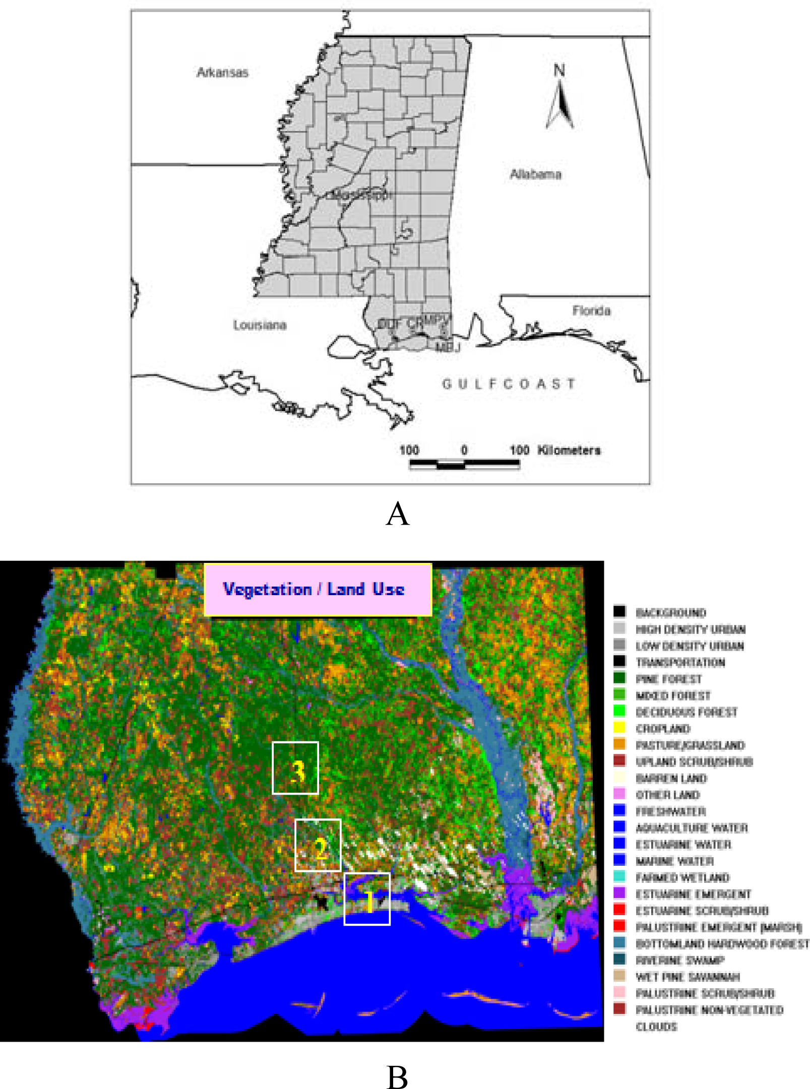
Location of Experiment

The experiment was conducted at 3 sites on the Mississippi Gulf coast (Figure 1a). The first site Navy Base is located near to Ocean Springs (Figure 1b) (30.22° N, 89.07° W). The site is a plain terrain with an average elevation of 9 m above mean sea level (AMSL). The second site is Harrison which is located about 15 kilometers away from gulf coast (30.52° N, 89.10° W) and has a mean elevation of 23 m AMSL. The third site is Wiggins located about 25 kilometers away from gulf coast (30.83° N, 89.15° W) with an average elevation of 10 m AMSL (Fig 1b). The major land-use type of Wiggins is Pine forest and mixed forest land, that of Harrison is Urban, cropland and pasture /grass land, while the land-use of Sea Bee base is high density urban, backflow water and deciduous forest. The vegetation comprises mixed and deciduous forest near the coast, and gradually changes to forest, pasture /grass land inside the coast. The sites are located normal to the Mississippi coast on the north and experience the sea breeze from south during the summer season. These locations were selected in the order of increasing distance from the coast so that the variations in atmospheric structure could be analyzed.

Equipment Used

In the present experiment a slow ascent GPS sonde is used for measurement of meteorological parameters in the Boundary layer and the free atmosphere above ABL. The Marwin GPS sonde receivers with meteorological payload were provided by the Naval Research Laboratories in the Gulfport. The GPS Sonde gives the location coordinates of the sonde directly as it ascends using the GPS navigation techniques. In addition to the GPS sonde, two meso-net micrometeorological towers at Harrison, West Worthom installed as part of NOAA UrBANet are used for wind turbulence measurements. These towers are equipped with Sonic anemometer, temperature, wind and humidity sensors at 2m, 10 m level and the data is regularly archived and available online ( http://dcnet.atdd.noaa.gov/) for dispersion research application.
During experiment time, upper air data from radiosonde observations at Slidell was also obtained to validate the GPS Sonde observations. A one week measurement programme was carried out during 25–29 June, 2007 at three locations. There was occasional thunder storm activity and the sky was often cloudy with occasional drizzle on June 27. The weather was dry on 28 and 29 June. The GPS sonde payload attached to Helium balloons were launched at 07:00, 13:00 and 18:00 LT on the experiment days.

Brief Description of the Modeling Aspects

Mesoscale Atmospheric Model

The Advanced Research Weather Research and Forecasting (WRF) mesoscale model version 2.2 developed by the National Centre for Atmospheric Research (NCAR) is used to simulate the wind flow pattern and other meteorological variables in the study area. The WRF-ARW is based on the Eulerain mass solver [19] and consists of fully compressible non-hydrostatic equations. The model prognostic variables include the three-dimensional wind, perturbation quantities of potential temperature, geo-potential, surface pressure, turbulent kinetic energy and scalars (water vapour mixing ratio, cloud water etc). The model vertical coordinate is terrain following hydrostatic pressure and the horizontal grid is Arakawa C-grid staggering. A 3rd order Runge-Kutta time integration is used in the model. The model has several options for spatial discretization, diffusion, nesting, lateral boundary conditions and physics parameterization.

Dispersion Model

A Hybrid Single-Particle Lagrangian Integrated Trajectory (HYSPLIT) model [20, 21] developed by Air Resources Laboratory, NOAA is used to simulate the dispersion of airborne pollutant releases. HYSPLIT computes simple trajectories to complex dispersion and deposition simulations using puff or particle approaches. The dispersion computation consists of three components: particle transport by the mean wind, a turbulent transport component, and the computation of air concentration. Pollutant particles are released at the source location and passively follow the wind field. The mean particle trajectory is the integration of the particle position vector in space and time. The turbulent component of the motion defines the dispersion of the pollutant cloud and it is computed by adding a random component to the mean advection velocity in each of the three-dimensional wind component directions. The vertical turbulence is computed from the wind and temperature profiles and the horizontal turbulence is computed from short-range similarity theory. The meteorological fields needed in the model are u,v,w (horizontal, vertical wind components), T(temperature), Z (height) or P (pressure), surface pressure (Po) and the optional fields moisture and vertical motion. These gridded three dimensional fields are linearly interpolated in space and time to the particle’s position. The advection of a particle or puff is computed from the grid scale three-dimensional velocity vectors obtained from the meso-scale model. A random component to the motion is added at each step according to the atmospheric turbulence at that time. The horizontal turbulent velocity components at any given time are computed from the turbulent velocity components at the previous time, an auto-correlation coefficient that depends upon the time step, the Lagrangian time scale, and a computer generated random component.
The lagrangian time scales TLw (vertical) = 100 s and TLu (horizontal) = 10800 s are assumed to be constant for convenience. These values result in a random walk vertical dispersion for most of the longer time steps. Turbulent mixing is calculated using a diffusivity approach based upon vertical stability estimates and the horizontal wind field deformation. The ratio of vertical to the horizontal turbulence (0.18) is used in the model. Pollutant concentrations are estimated as integrated mass of individual particles as they pass over the concentration grid which is a matrix of cells, each with a volume defined by its dimensions. The details of the model equations and the dispersion methods are detailed in the technical paper [20].

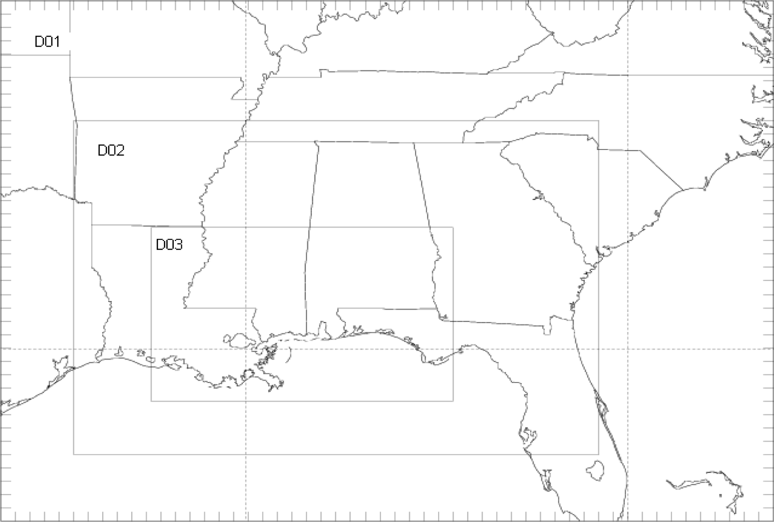
Model Domains and Initialization

WRF model is configured with 3 nests with grid resolutions of 36, 12 and 4 km, the 2nd and 3rd are two-way interactive nests. The outer domain covers the South-central US and the surrounding Atlantic Ocean to capture the dynamics that might influence the circulation in Mississippi. The inner finer grid (4 km) covers the Mississippi Gulf Coast off Louisiana above the Gulf of Mexico. The coarse domain has the size of 54 × 40 grid points while the finer domain has 187 × 118 grid points (Fig. 2). All the domains contain 32 vertical levels with 12 levels in the lower atmospheric region (below 800 hPa). The USGS topography and vegetation data (25 categories) and FAO Soils data (17 categories) with resolutions 5m, 2m and 30sec (0.925 km) are used to define the lower boundary conditions for domains 1, 2 and 3 respectively. The initial and lateral boundary conditions are obtained from National Centers for Environmental Prediction (NCEP) Final analysis (FNL) data as pressure level input. This data contains horizontal, vertical wind, geopotential height, pressure, temperature, specific humidity, cloud cover at several vertical levels up to troposphere, and soil moisture and soil temperature. The top of the model is selected as 50 hPa. The boundary conditions to the model are given from the above data at every 6 hour interval and the model is integrated for 2 days (48 hours) starting on 00 UTC 28 June.
The surface layer variables are defined from similarity theory and PBL fluxes are calculated using the non-local turbulence closure model (YSU scheme) [22]. The NOAH (National Centers for Environmental Prediction, Oregon State University, Air Force, and Hydrologic Research) land surface model is used for the treatment of soil thermal and moisture processes. Atmospheric radiation calculations are performed every 30 minutes accounting for the long wave and short wave processes that interact with the atmosphere, cloud/moisture and the surface [23,24]. Atmospheric moisture in different forms (water vapor, cloud water, rain, snow, ice) is calculated using WRF single-moment 3-class (WSM3) simple ice scheme [25]. For the outer nests (domains 1, 2) a cumulus parameterization scheme [26] is used for large-scale convection. A relaxation lateral boundary condition is used for the outer domain while time dependent later boundary conditions are used for inner domains. Different options used in the WRF model are detailed in Table 1.

Dispersion Simulation

Dispersion simulation is done over a range of 100 km around the sources. A horizontal grid of 4° × 4° with resolution of 0.01° × 0.01° (roughly 1km × 1km) and with seven vertical levels 50 m, 100 m, 200 m, 400 m, 750 m, 1000 m, 3000 m above ground level (AGL) is considered in HYSPLIT dispersion model. Pollutant concentrations are sampled and averaged every 15 minutes. Among a cluster of industrial elevated point sources located along the MS coast, four major sources are considered in the present study. These are Mississippi Power Company-Plant Jack Wa (MPJ), Chevron Products Company-Pascagoula Oil Refinery (CR), Mississippi Power Company- Plant Victor (MPV) and Dupont Delisle Facility (DDF) (Fig.1a, Table 2). Emissions from each facility are considered to assign pollutant mass to each virtual particle represented in the HYSPLIT model. SO2 is considered as the pollutant species from all the sources. No seasonal or diurnal variations in the load factor are considered in the present study. The pollutant plume is treated as top-hat puffs in the horizontal and particle in the vertical.
A total of 500 particles or puffs are released during one release cycle with a maximum of 10000 particles permitted to be carried at any time during the simulation (Table 3). The time step is chosen such that a particle transits 0.75 grid cell distance in one advection step. The turbulence mixing is computed using a short-range diffusivity approach based upon vertical stability estimates. The turbulent velocities are computed directly from the stability parameters, either the heat and momentum fluxes, if available, or derived from the wind and temperature profiles. The puff dispersion is treated as linear with time. Ground level concentrations are computed as averages for the lowest 50 m within each horizontal grid cell.

Results

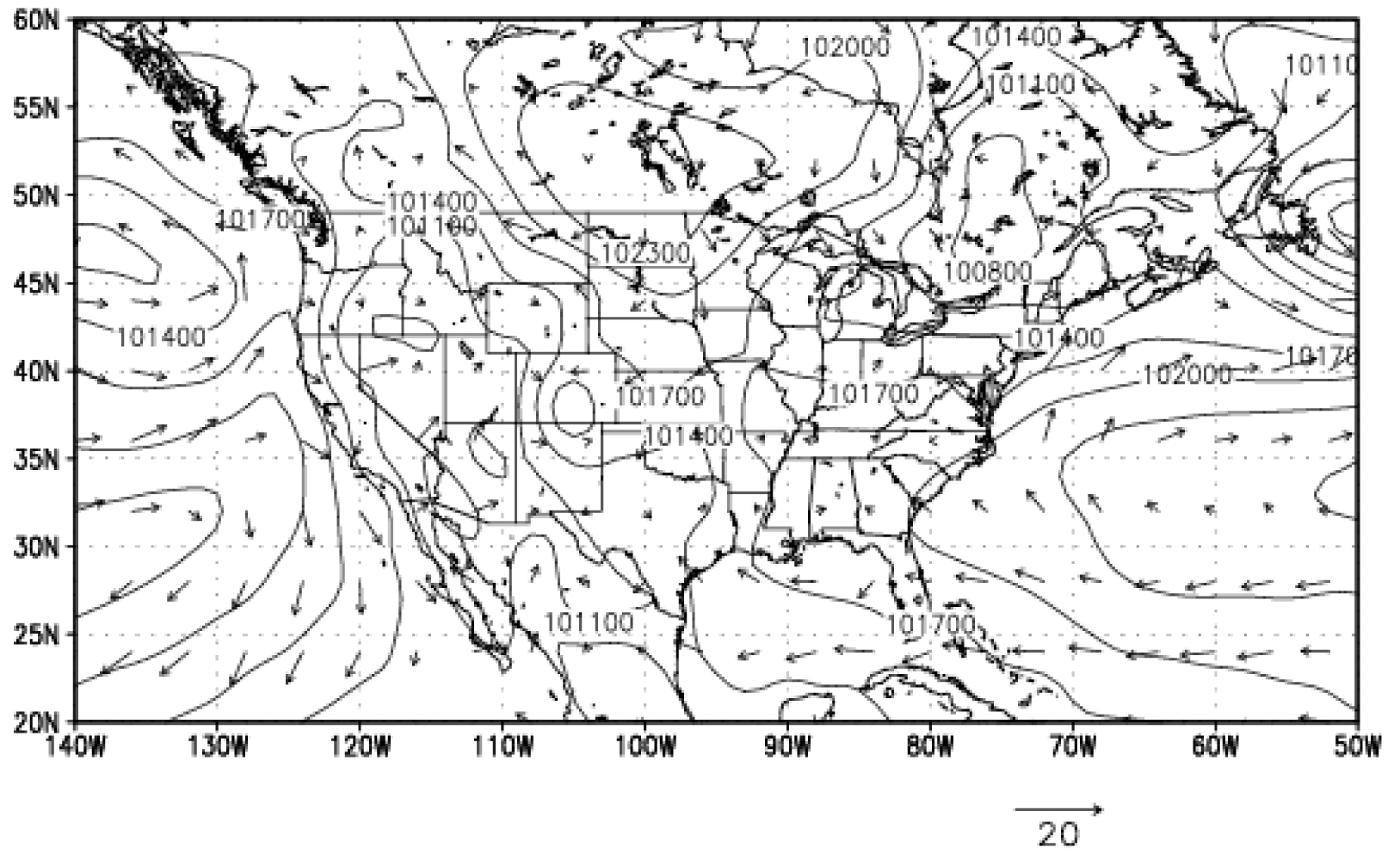
Synoptic Meteorological Conditions

The synoptic weather chart drawn from the FNL analysis during the experiment time is shown in Figure 3. It shows the sea level pressure and winds for 28 June 2007.
Westerly winds over the United States with low pressure conditions over the western parts and high pressure conditions over the rest of the US are seen. The morning winds (i.e., corresponding to 12Z) are north easterly and gradually change to south westerly in the afternoon time (i.e., corresponding to 00Z). On June 28 a high pressure ridge developed over the central and south eastern US.

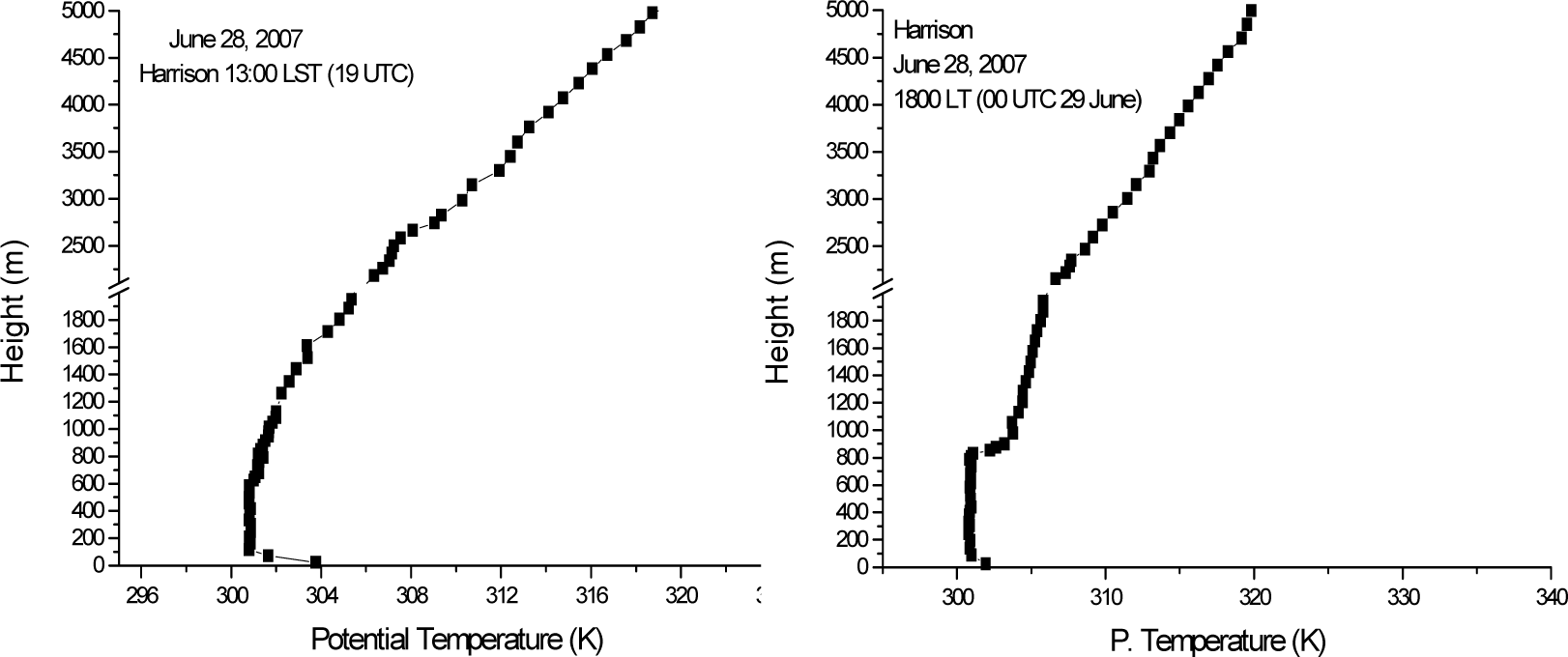
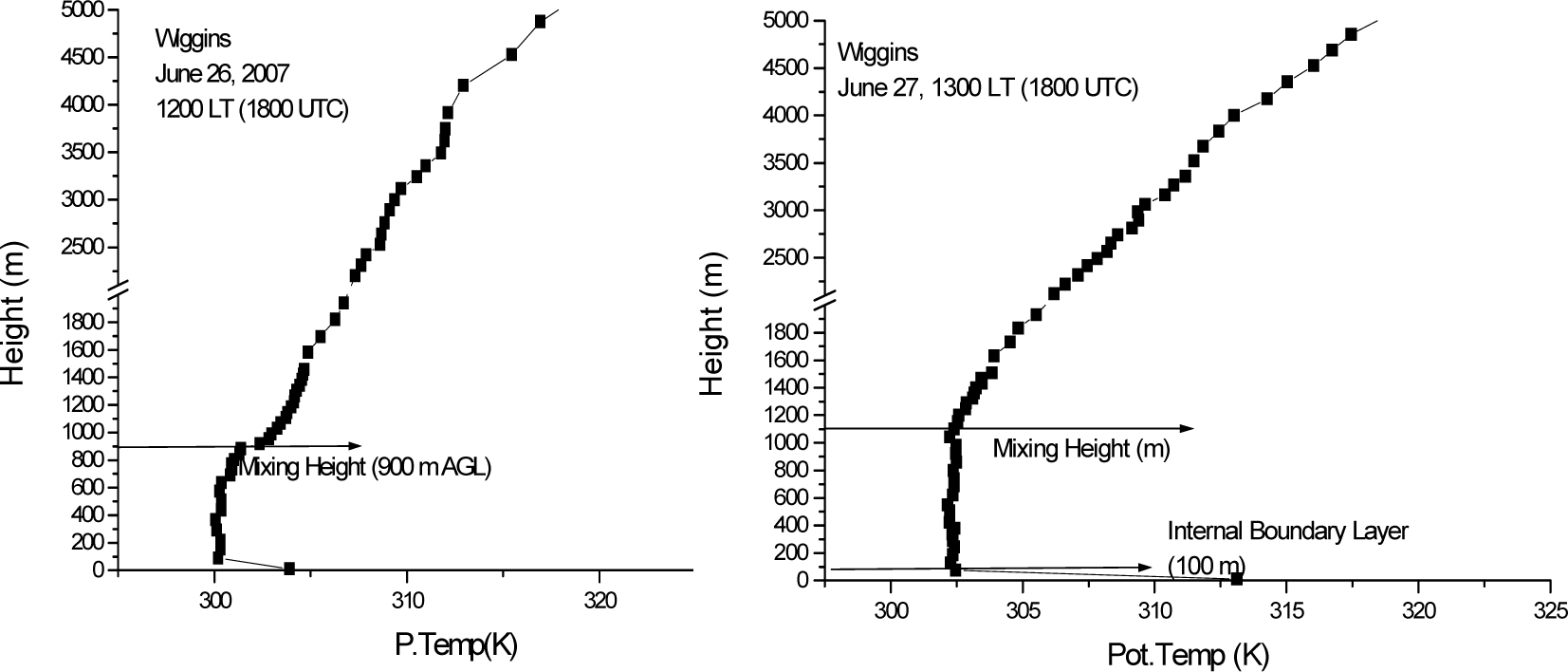
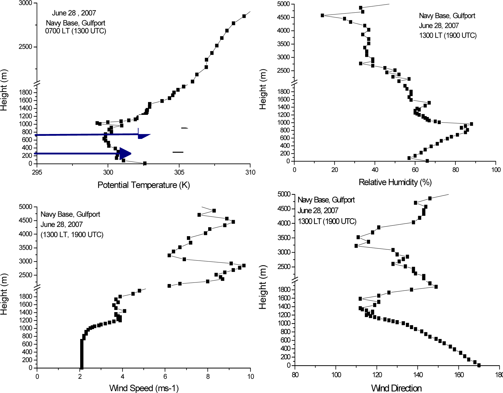
Wind and Temperature Profiles from GPS Sonde

Data of Raidosonde soundings at 00Z (1800 LT on the previous day) and 12Z (06 LT) are obtained from NWS, Slidell observatory. This upper air data is used to validate the GPS Sonde profiles in the experiment for the trends of wind, temperature, relative humidity up to a height of 15 km. The profiles are found to agree for the comparison times (not shown).
The profiles of temperature from GPS Sonde for each of the locations are analysed separately at different times. Profiles of temperature from GPS Sonde at Sea Bee base show a developing boundary layer in the morning, convective mixing layer in the noon, and shallow unstable layer near the ground in the evening conditions. The profiles are different on the different days due to variation in the sunshine, cloudiness and rain formation. Cloud formation and occasional rain were noticed on 26th June 07. A well mixed layer during daytime is formed on 28th noon (Fig. 4).
Fair weather prevailed on 27th and 28th June. The profiles on 27th afternoon indicate a steep shallow unstable layer near the coast indicating the internal boundary layer formation adjacent to the coast. The height of this IBL is about 100 m AGL. At Harrison the profiles were good on 28th June (Fig 5). A well developed PBL is seen at Harrison on 28th at noon 13:00 LT, the height of this PBL is about 900 m AGL. Within this PBL a steep unstable layer exists above the ground to a height of roughly 200 m. This can be recognized as the IBL at Harrison. Towards the evening this IBL disappears and the whole PBL is marked with well mixed layer.
At Wiggin’s air base the profiles indicate formation of steep unstable layer and a neutral layer during the convective daytime conditions. The depth of the unstable layer is about 100 m. The mixing layer depth reaches about 900 m on 26 June, and 1100 m on 27 June (Figure 6.) as the cloud cover decreased on 27th.
During the sea breeze time at Seabee base (Navy base), the profiles at 13:00 LT for potential temperature, relative humidity, wind speed and wind direction are examined. The profiles for temperature and RH clearly show a shallow unstable layer near the ground (Fig. 7). Temperature distribution is gradually altered and a shallow unstable layer marked with steep lapse rate is seen up to 150 m AGL and a mixed layer up to 500 m AGL at 13:00 LT.
Similarly the profiles at Harrison during the sea breeze time show a steep and shallow unstable layer. Greater wind shear associated with fluctuation in the wind speed profiles is noticed at 13:00 LT during the sea breeze time.

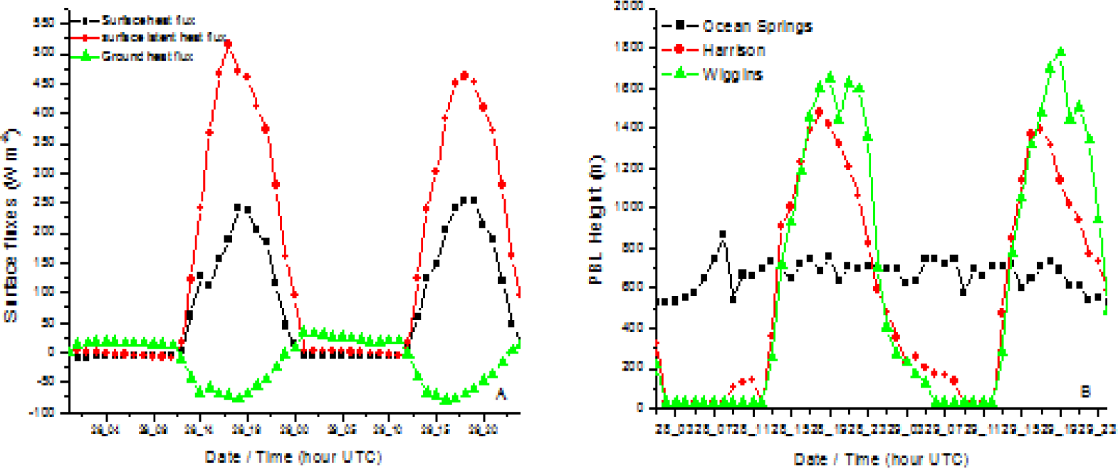
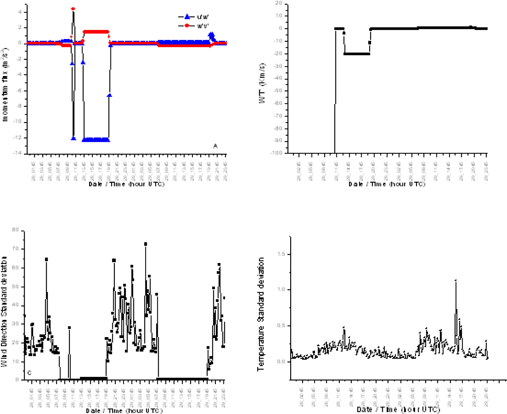
Diurnal Variation in Surface Layer Parameters

The micrometeorological tower observations of the NOAA AWS at Harrison are shown in Fig 8.
Eddy fluxes are calculated from sonic anemometer fast response sensor data. The eddy correlation fluxes are positive maximum during noon and minimum during night conditions which indicate the diurnal PBL turbulence variation. All the variables show diurnal variation due to PBL development and decay. Maximum fluctuation in eddy momentum flux, eddy heat flux, wind direction and temperature are noticed coinciding with the circulation change at Harrison at 03 UTC during night time and at 14 UTC during daytime. The variables reach their peak values around the noon. The standard deviation of the variables temperature and wind direction vary diurnally and attain peak in the morning and afternoon conditions which indicates greater turbulence in the lower atmosphere around the daytime time.

Meteorological Model Results

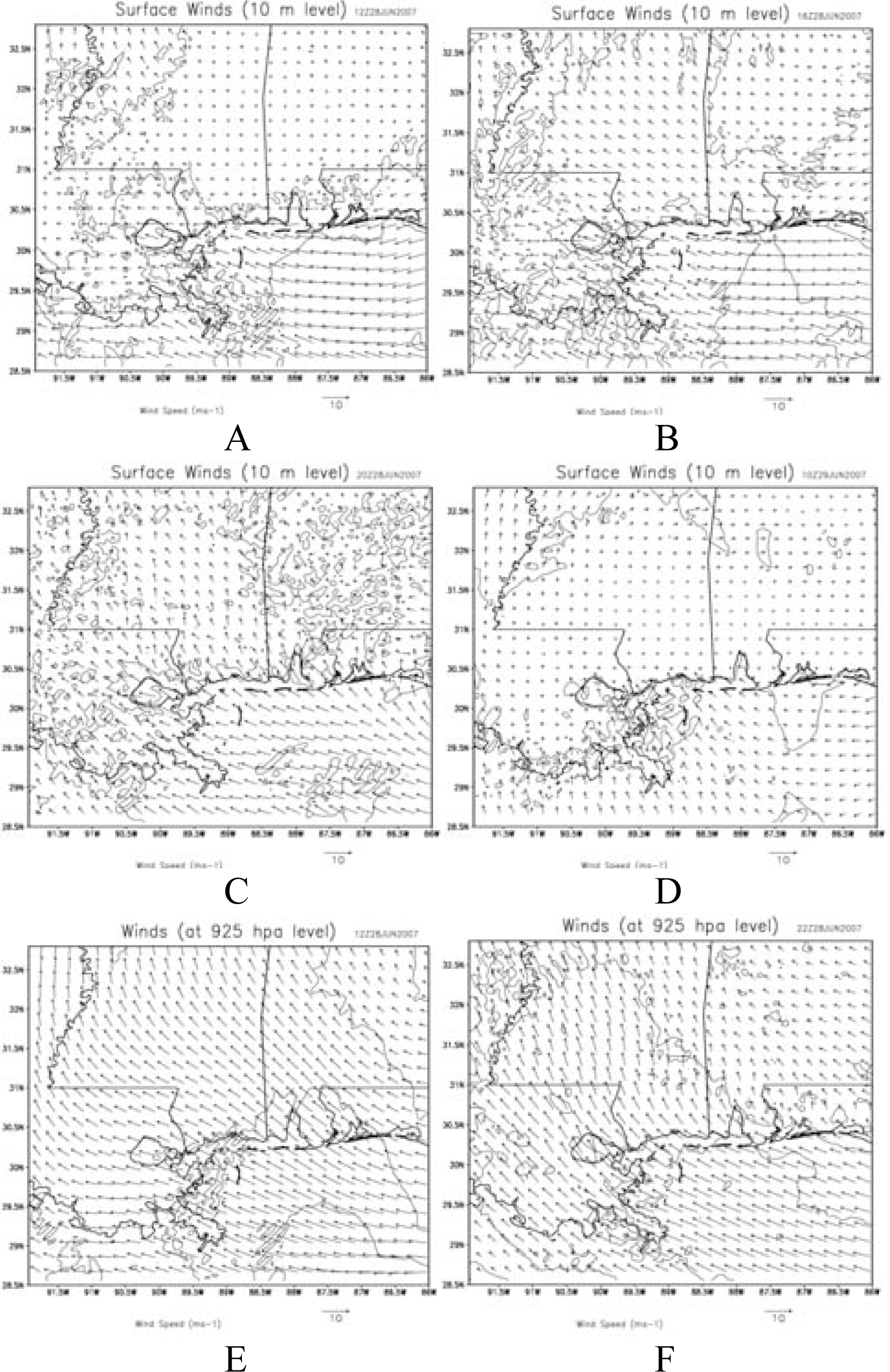
Horizontal Flow Field

Simulated flow pattern in the outer domain (domain 1) is southeasterly in the lower troposphere and agrees with NCEP NAM Eta analysis data (not shown).
Simulation from the inner fine grid domain indicates a diurnally varying horizontal wind field in the lower atmosphere. Simulated horizontal wind field at 10 m level is shown in Fig 9 corresponding to 0600, 1000, 1400 LT on June 1, 2006, and 0400 LT on the next day. The flow pattern primarily consists of a coupling of the local flow with the largescale flow. Development of sea breeze (SB) circulation during the day time and land breeze (LB) during the night conditions is noticed adjacent to the coast. Simulated meteorological fields by WRF model show the influence of synoptic flow in the morning hours. The flow is altered at the lower levels by the interaction of local sea-breeze (SB) circulation in the course of the day. Similarly the flow is modulated in the night by the land breeze (LB) forming due to relative cooling of land.
Simulated surface level flow in Mississippi is predominantly easterly during morning time and is influenced by the complex coastline of Louisiana at the coast (Fig. 9a). The flow gradually became strong southerly and southeasterly by the onset of sea breeze at the Mississippi – Louisiana coast (Fig 9b–9c). Horizontal extent of the onshore flow increased towards the late evening time. Owing to the relative cooling of the land, decay of land-sea temperature gradient and formation of stable surface layer in the night the sea breeze weakens. Land breeze developed during the night due to a reverse temperature gradient establishment, and is noticeable by weak winds across the Mississippi coast (Fig. 9d). However, it could not fully establish like sea breeze due to the opposing synoptic winds. Day time flow pattern on the following day shows development of sea breeze at the same time (not shown) which is seen by comparing the midday flow patterns of the days studied. Wind flow in the upper levels up to 1 km (∼925 hPa level) is examined as it would influence the pollutant trajectory pattern for elevated releases. Circulation at 925 hPa level is predominantly led by the synoptic flow and is not altered by topographic effects until around noon (Figs. 9 e, f). Around noon influence of Sea breeze is noticeable with significant onshore flow. Sea breeze interaction with synoptic flow is seen to continue till late evening and flow over most of the domain is covered by sea breeze in the late evening. Unlike the surface wind, LB is not noticed at 925 hPa level except a slight change in wind direction in the late night. As in the case of surface flow, the next day’s flow pattern at 925 km is similar to the flow simulated in the first day. Sea breeze occurrence is noticeable on the next day also around noon.
To validate the simulation comparison is made with the North American Mesoscale (NAM) analysis fields which are available at 3 h intervals over much of North America from NCEP. It is seen that the WRF wind field at the surface and 1 km levels reasonably agrees well with NAM analysis data at the corresponding times (Fig. 10). Off-shore and easterly winds during the night / early morning hours, gradual shift in flow from easterly to southeasterly and southerly direction (onshore winds) could be identified from the simulation as well as analysis fields.
Similarly a good comparison is found with the NAM data for the other parameters such as surface temperature, humidity and divergence patterns. While night temperature is lower in central Mississipi and Alabama (∼295 K) it gradually increased to 299 K towards the coast and western MS and the daytime temperature was about 3002 K uniform throughout MS. Convergence is seen over much of MS at 1km level during the daytime while divergence is seen at the coast and its adjacent land portion during the late evening and night hours. Higher humidity (72–86%) is found at the coast and its adjacent land portion during afternoon and night hours while very low humidity (44–58%) prevailed in the forenoon.

Vertical Cross-Section of Simulated Variables

Vertical cross-section of simulated horizontal winds, potential temperature, divergence/ convergence and vertical winds in north-south vertical section across the Mississippi coast are studied as they determine the vertical mixing and air concentrations. The time changes in the lower atmospheric circulation with corresponding changes in the temperature are shown in Fig. 11 in which grid points 1–30 indicate water surface over sea and grid points above 30 indicate land region.
A shallow land breeze circulation over a depth of 200 m is noticeable in the morning time over the land (not shown). Development of sea breeze is noticeable at 1600 LT (Fig. 11). The lowest region up to 800 m AGL is dominated by southerly sea breeze flow which gradually advances further north (inland) in late evening hours. The grey shade indicates divergence / convergence pattern associated with LB/SB currents in Fig.11. Convergence (< −1.5×10⁻⁵s−1) is associated with the vertical ascents. Divergence is associated with return flow aloft and associated subsiding motion. Sea breeze front formation is noticeable at the zone of converging winds and strong vertical wind velocity. Around the location of sea breeze front maximum vertical winds are noticeable with a magnitude of up to 20–25 cm s−1 and with a corresponding vertical motion of 30.0 dPa s−1. The vertical winds associated with subsiding currents have maximum vertical winds of −4.5 cm s−1. Strong convergence is seen at the location of the front and upward diverging motion associated with return currents. Contours of potential temperature across the coast (Fig. 11) indicate stably stratified atmosphere over the water portion and unstable thermal stratification over the land portion. The unstable layer is seen to extend up to a few tens of kilometers inside the coast and can be recognized as the internal boundary layer at the coast. The height of the IBL at 1600 LT is about 100 m just near the coast and gradually increases to 800 m inland until it merges with the generic boundary layer farther inland.
From the plots of simulated PBL height, it is seen that a stable boundary layer forms overland in the night and morning conditions (Fig. 12a). The height of the stable boundary layer is about 100 m to 300 m. In the course of the day to progressive heating and convection, the PBL grows and the PBL height is about 1400 m at the coast and 2000 m inland in the noon (Fig. 12 b). When the sea breeze sets in the PBL height along the coast is seen to sharply fall to 600 m to 1000 m up to a few tens of kilometers indicating development of IBL (Fig. 12c).
Diurnal evolution of simulated and observed surface meteorological variables is shown in Fig.13 for 10-m wind speed, direction and 2m air temperature and relative humidity. These plots show the model could reproduce the observed trends in the surface parameters. Shift in the wind direction, rise in wind speed, rise in surface humidity and a fall in the temperature as noticed from observations at the coast could be simulated by the model. The model values are smoother and there is a lag of approximately 1 hour in the model trends of various surface parameters. The model vertical profiles for potential temperature, wind speed and wind direction for the grid corresponding to Harrison site are compared with the GP Sonde observations on 28 June 07 (Fig. 14). The model values are grid and time averaged and hence is smoother than the GPSonde profiles which exhibited significant vertical fluctuations. However the model could bring out the vertical trends in the variables as can be seen from observational comparison.
The diurnal surface turbulent fluxes simulated by WRF model for Harrison location are shown in Fig. 15a. It can be seen that the latent heat flux is much higher than the sensible and ground heat fluxes as the site is very near to the coast. As in the case of observed eddy heat flux the maximum in the model sensible heat flux arises at around 15 UTC on 28 June. The PBL vertical growth is maximum at Wiggins (about 2000 m AGL), followed by Harrison (about 1500 m AGL) and Ocean Springs (about 700 m AGL) (Fig. 15b). There is no much variation in the diurnal PBL height for Ocean Springs which is located just at the sea. The model, as well as observations, show a mixing height of about 1000 m at Harrison location and a shallow unstable layer (∼150 m AGL) near the ground. Similarly the model values as well as the observations indicate the lower level inversion in the morning conditions. Thus the WRF model could reproduce the observed trends in the vertical structure of the atmosphere and the diurnal trends in the surface parameters in the coastal region.

Dispersion Simulation Results

Dispersion calculation is made with particle dispersion model HYSPLIT using the meteorological fields simulated by WRF mesoscale model as detailed in the previous section. Dispersion simulation is made in a range of 100 km around the release points. Particles are released at regular intervals in the HYSPLIT model from the four elevated sources.

Simulated Air Mass Trajectories and Particle Positions

Simulated forward particle trajectories from HYSPLIT model using WRF wind fields are presented in Fig.16. The air mass trajectory follows the stream line. Trajectories originating at different starting times from the point sources are seen to travel to different locations on the Mississippi coast indicating the influence of time varying circulation. Initially the synoptic flow steers the trajectories in the northwest direction (Fig.16), latter they are influenced by the sea breeze circulation and move to north (Fig.8b, c). In each case trajectories indicate influence of the local flow near the coast and the large-scale flow farther away. Trajectories are noticed to confine to the lower atmospheric region below 2 km. The vertical movement of trajectories is noticed to follow the diurnal variations in mixing height variations.
Vertical cross-sections of integrated particle positions in the direction of the plume are shown in Fig. 17. They represent the vertical dispersion of the particles at different times during the day. In the night conditions, stable thermal stratification prevails and the particle vertical mixing is limited to the lower 0.5 km region. The deep plume in the night condition shows the particles advected earlier during the day time. During the daytime the boundary layer grows vertically and there is enhanced mixing and vertical spread of the particles as noted from Fig.17a. Particles are densely distributed within a layer of about 200 m above ground level, especially during the late night associated with stable conditions.
It is seen that particles are more densely distributed during morning stable conditions (10 UTC/ 4 LT) than during the daytime unstable conditions (22 UTC/ 16 LT). The vertical distribution of particles is higher in the daytime than during the night time. A major number of particles reached up to 2000 m AGL in the convective daytime condition. The horizontal particle distribution also indicates variations according to the variations in mixing height across the coast.

Plume Distribution

Simulated SO2 concentration fields averaged every 15 min for the lowest 50 m layer are presented in Fig.18 (a,b,c and d) for the periods ending at 10, 17, 27 and 37-hr respectively after the beginning of calculation.. The plume evolution can be noticed to follow the simulated diurnal wind flow pattern. The horizontal spread of the plume is noticed to vary in the course of day due to changes in stability and wind and also due to spatial variations in the wind field. The plume direction was to the west at night time (Fig 18a), to the northwest in the noon (Fig 18b), to the north (Fig 18c) in the late evening / night conditions and to the northeast in the morning next day (Fig 18d).
The plume gradually turns to land region in the afternoon on the sea breeze development and completely stays on land with full sea breeze establishment. It is narrow during the stable morning conditions, and disperses over a wide area during the transition of land-breeze to sea breeze as seen from a widely spread plume at sea-breeze incidence time. On full development of sea breeze, the plume is narrow in the region of sea breeze influence and is wide spread further downwind. This is attributed to the enhanced turbulence generation at the sea breeze frontal zone. During the transition times i.e., during the onset of LB or SB distinctly different patterns of dispersion can be noticed, one near the source in the direction of local circulation and the second due to earlier spread releases in the direction of the mesoscale flow. Ground level concentration distribution is examined in a 100 km range from the source locations. During the morning time releases occur within a stable boundary layer, the ground level concentration near the release locations (< 5 km) is 0.1 μg m−3 which falls to 0.01 μg m−3 at distance rage of 20 to 50 km and 0.001 μg m−3 in 50–100 km in the southeast direction (Fig.18 a). During sea breeze the concentration drops to a low value of 0.01 μg m−3 over large area in the plume direction. After the incidence of sea breeze the maximum concentration (0.1 μg m−3) occurs at distance ranges up to 40 km. The contours corresponding to the value of 0.10–0.01 μg m−3 are extending to large downwind distances. This is due to the formation of shallow mixing layer and relatively low wind speeds in the forward direction of the sea breeze flow, thus reducing the vertical diffusion and horizontal transport of pollutants.
The plume pattern in the morning time gives two distinctly different concentrations i.e., 0.1 μg m−3 in the direction of the plume up to 20 km (southeast direction) and 0.0001 μg m−3 behind the plume due to the dispersion in the earlier release in the night conditions (Fig. 18 d). Again on the next day (June 29) on the setting of sea breeze a wide spread dispersion is noticeable with maximum concentrations of 0.01 μg m−3 (not shown).
Thus it is noticeable that the concentrations are higher during the morning stable conditions and during the afternoon sea breeze time. The highest SO2 concentration simulated by the HYSPLIT model is 0.1 μg m−3. This occurs during two conditions, one in the stable morning time up to 20 km in the west direction (Fig. 18a) and the second during the sea breeze time up to about 40 km in the north (Figs.18b). The second highest concentration 0.01 μg m−3 occurs during most of the day.
Figure.19 shows the simulated SO2 concentrations sampled at the model grid corresponding to the monitoring stations Natchz, Pascagoula, Cleveland, Meridian, Gulfport and Jackson County respectively in the MS. It is to be noted that the actual SO2 concentration levels would show both background and longer range contributions from other nearby sources not included in the model calculations while the model only shows contributions above the background. The monitoring data for the simulation time are not available hence the model values at different locations are used merely to compare the diurnal trends in the simulated values.
Model calculations show diurnal variation in concentration. Concentration at most locations indicates a bimodal distribution with a peak in concentration during stable morning and in the afternoon times. The concentration peaks occurred at slightly different times at different locations due to the variation in the visiting time of plume at different locations.

Summary and Conclusions

The field meteorological experiment conducted at three different locations across the MS Gulf coast during the summer season has given opportunity to gain an insight on the PBL characteristics across the coast and to measure the mixing depth and its diurnal variation across the coast. Mixing depth increased progressively from coast to inland, the PBL height was 600–700 m at Sea Bee base , 1000–1500 m at Harrison and 1400–2000 m AGL inland. Boundary layer field experiment reveals formation of thermal internal boundary layer adjacent to the coast, the height of this shallow IBL is about 100 m at the coast, and 300 m about 15 km inland. Wind speeds increase during the sea breeze time, and significant change in the meteorological parameters is noticed at the sea breeze occurrence. A meso-scale model WRF with triple nested domains was used to simulate the meteorological parameters in the MS Gulf coast. The experiment data was used to validate the WRF model which simulated the flow and PBL structure in the region. The simulation results closely agreed with the GPS Sonde observations. The model could bring out the observed vertical structure and the mixing depth variations across the coast although there was a slight lag in the simulated daytime peak values. The WRF model could reproduce the flow and many of the observed characteristics of the coastal ABL and hence could be useful in dispersion / air quality studies in the region. Both the model and the observations indicate shallow unstable layer and sea breeze incidence at the coastal location. The dispersion simulation using HYSPLIT model with WRF data has shown the expected diurnal variations in the plume direction and concentration distribution. However exhaustive studies with WRF and Community Multiscale Air Quality (CMAQ) Model need to be conducted to understand the ozone transport and pollution episodes in the region which require generation of high resolution emission inventory for the study region. The present experiment has given valuable data base on the boundary layer structure across the coast useful for validation of the numerical models used in dispersion assessment.
Figure 1:. Location of the study region (a) and Vegetation / Land use of the Mississippi Gulf coast region (b). The experimental locations are Sea bee base (1), Harrison (2) and Wiggins (3).
Ijerph 05 00484f1
Figure 2:. Modeling domains used in WRF
Ijerph 05 00484f2
Figure 3:. Sea level pressure and surface winds at 10m level at 00Z 28 June 2007.
Ijerph 05 00484f3
Figure 4:. GPS sonde potential temperature profiles for Sea Bee Base for 27 and 28 June 08.
Ijerph 05 00484f4
Figure 5:. Vertical profiles of potential temperature at Harrison site on June 28.
Ijerph 05 00484f5
Figure 6:. Vertical profiles of potential temperature at Wiggins site on June 26 and June 27 at 13:00 LT.
Ijerph 05 00484f6
Figure 7:. Profiles of potential temperature, R.H, Wind speed and direction during sea breeze time at Sea Bee Base.
Ijerph 05 00484f7
Figure 8:. Diurnal trends of u/v momentum flux (A), eddy heat flux (b) and wind direction standard deviation (c) and temperature standard deviation (d) at Harrison site.
Ijerph 05 00484f8
Figure 9:. Simulated wind pattern in the MS Gulf coast region for 28–29 June, 2007. Panels a,b,c,d-for the surface wind and panels e,f-for winds at 925 hPa (∼1km) level.
Ijerph 05 00484f9
Figure 10:. Observed wind flow pattern from NCEP NAM analysis for 28–29 June 2007. Panels a,b,c,d-for surface wind and panels e, f-for winds at 1km.
Ijerph 05 00484f10
Figure 11:. Vertical section of Potential temperature (K) and circulation vectors (ms−1), divergence (1.0e–05 s−1) and vertical motion (s−1) for a south-north vertical-section at 1600 LT on June 28, 2007.
Ijerph 05 00484f11
Figure 12:. Simulated PBL height (m) at 0600 LT (A), 1200 LT (B) and 1600 LT (C) on June 28, 2007.
Ijerph 05 00484f12
Figure 13:. Simulated and observed 10 m wind speed (A), 10 m wind direction (B), 2m relative humidity (C) and 2m air temperature (D) for the model grid at Harrison site from 18:00 LT June 28- 18:00 LT, June 30.
Ijerph 05 00484f13
Figure 14:. Simulated and observed vertical profiles of potential temperature at 07 UTC (a), 13 UTC (b), wind speed at 07 UTC (c), 13 UTC (c) and wind direction at 07 UTC (e), 13 UTC (f) for the Harrison location
Ijerph 05 00484f14
Figure 15:. WRF simulated surface fluxes at Harrison (a) and simulated boundary layer height at Ocean Springs, Harrison and Wiggins.
Ijerph 05 00484f15
Figure 16:. Forward trajectories of the particles starting at 00 UTC (a) and at 12 UTC (b) on 28 June from the four emission sources [Green – Gulfport (height of release– 115 m); Red – Gulfport (height of release - 45 m); Cyan – Pascagoula (height of release 54 m); Blue – Pascagoula (height of release 45 m)]
Ijerph 05 00484f16
Figure 17:. Vertical section of particle positions simulated by the Hysplit model for continuous emissions from the four locations at a) 22 UTC 28 June and b) 10 UTC 29 June.
Ijerph 05 00484f17
Figure 18:. SO2 concentrations (g m−3) averaged for 1 hour intervals in the lowest 50 m computed by Hysplit model for A)10 UTC 28 June, B)17 UTC 28 June, C)03 UTC 29 June and D)13 UTC 29 June
Ijerph 05 00484f18
Figure 19:. Simulated SO2 concentration at 5 model grids corresponding to 1) Natchz, 2) Pascagoula 3) Cleveland 4) Meridian 5) Gulfport and 6) Jackson County
Ijerph 05 00484f19
Table 1:. Details of the physics and grid configuration used in WRF model
DynamicsPrimitive equation, non-hydrostatic

Vertical resolution32 levels

DomainsDomain1Domain2Domain3
Horizontal resolution36 km12 km4 km
Grid points54 × 40109 × 76187 × 118
Domains of integration93.0 W – 78.05 W91.74 W – 81.92 W90.28 W – 84.77 W
27.16 N – 34.45 N28.5 N – 34.45 N29.38 N – 32.54 N
RadiationDudhia (1989) scheme for short wave radiation, Rapid radiative transfer model (RRTM) for long wave radiation
Surface processesNoah Land surface model
Boundary layerYonsei State University (YSU) PBL scheme
Initial, boundary conditions, Sea surface temperatureNCEP FNL analysis data
ConvectionKain and Fritsch (1993) scheme on the outer grids domain1, domain2
Explicit moistureWSM3 class simple ice (SI) scheme
Table 2:. Sources of elevated release considered for the Hysplit computations
LocationStack Ht(m)Stack Diameter Ds (m)SO2CONOX
Gulfport115.13.8511280.87021.1285.5
Pascagoula54.11.351742.81367.632.4
Escatawpa105.010.2312522.24742.9299.1
Passchritian45.03.01270.53565.63263.5
Table 3:. Hysplit dispersion model configuration
Grid Centre30.5 N, -89.5 L
Vertical resolution7 Levels – 50, 100, 200, 500, 1000,2000, 5000
Horizontal Grid2 × 2 degree
Horizontal resolution0.01 × 0.01
Turbulence MethodStandard Velocity Deformation, Vertical diffusivity
MeteorologyWRF Simulated hourly meteorological fields
Number of release particles per cycle500

Acknowledgments

Authors thank for the support of the Atmospheric Dispersion Project (ADP) funded by the National Oceanic and Atmospheric Administration through the U.S. Department of Commerce (Silver Springs, MD); Contract #NA06OAR4600192. The authors thank the National Center for Atmospheric Research (NCAR) for the analysis data and the Mississippi Department of Environmental Quality for providing the emission data of the elevated point sources used in the study. Special thanks are due to the Navy Sea Bee Base for providing the GPS Sonde equipment and for the support in conducting the meteorological experiment. Authors gratefully acknowledge the NOAA ARL for the tower observations at Harrison and for providing the HYSPLIT dispersion code used in the study.

References

  1. Garratt, JR. The Atmospheric Boundary-Layer; Cambridge University Press: UK, 1992; pp. 1–316. [Google Scholar]
  2. Liu, H; Chan, JCL; Chang, AYS. Internal boundary layer structure under sea-breeze conditions in Hong Kong. Atmos. Env 2001, 35, 683–692. [Google Scholar]
  3. Luhar, AK. An analytical slab model for the growth of the coastal thermal internal boundary layer under near-neutral onshore flow conditions. Bound. Layer. Meteor. 1998, 88, 103–120. [Google Scholar]
  4. Stull, RB. An Introduction to Boundary Layer Meteorology; Kluwer Academic Publishers: Dordrecht, 1988; p. 666. [Google Scholar]
  5. Boybeyi, Z. Sethu Raman.: Numerical Investigation of Possible Role of Local Meteorology in Bhopal Gas Accident. Atmos. Env 1995, 29(4), 479–496. [Google Scholar]
  6. Pielke, RA; McNider, RT; Moran, MD; Moon, DA; Stocker, RA; Walko, RL; Uliasz, M. Regional and mesoscale meteorological modeling as applied to air quality studies. In Air Pollution Modeling and Its Application. VII; Van Dop, H, Steyn, DG, Eds.; Plenum Press, 1991; pp. 259–290. [Google Scholar]
  7. Pielke, RA; McNider, RT; Segal, M; Mahrer, Y. The use of a mesoscale numerical model for evaluations of pollutant transport and diffusion in coastal regions and over irregular terrain. Bull. Amer. Met. Soc 1983, 64, 243–249. [Google Scholar]
  8. Jin, H; Raman, S. Dispersion of an elevated release in a coastal region. J. Appl. Meteor. 1996, 35, 1611–1624. [Google Scholar]
  9. Kotroni, V; Kallos, G; Lagouvardos, K; Varinou, M; Walko, R. Numerical simulations of the meteorological and dispersion conditions during an air pollution episode over Ahtens, Greece. J. Appl. Meteor. 1999, 38, 432–447. [Google Scholar]
  10. Lu, R; Turco, RP. Air Pollutant transport in a coastal environment II. Three-dimensional simulations over Los Angeles Basin. Atmos. Env. 1995, 29, 1499–1518. [Google Scholar]
  11. Monti, P; Leuzzi, G. A numerical study of mesoscale airflow and dispersion over coastal complex terrain. Int. J. Environ. and Poll 2005, 25(1), 239–250. [Google Scholar]
  12. Uliasz, M. The Atmospheric Mesoscale Dispersion Modeling System. J. Appl. Meteor 1993, 32, 139–149. [Google Scholar]
  13. Segal, M; Pielke, RA; Arritt, RW; Moran, MD; Yu, CH; Henderson, D. Application of a mesoscale atmospheric dispersion modeling system to the estimation of SO2 concentrations from major elevated sources in southern Florida. Atmos. Env. 1988, 22(7), 1319–1334. [Google Scholar]
  14. Physick, WL; Abbs, DJ. Flow and Plume Dispersion in a Coastal Valley. J. Appl. Meteor 1992, 31, 64–73. [Google Scholar]
  15. Liu, H; Chan, JCL. An investigation of air-pollutant patterns under sea-land breezes during a severe air-pollution episode in Hong Kong. Atmos. Env 2002, 36, 591–601. [Google Scholar]
  16. Liu, H; Chan, JCL. Boundary layer dynamics associated with a severe air-pollution episode in Hong Kong. Atmos. Env. 2002, 36, 2013–2025. [Google Scholar]
  17. Ohashi, Y; Kida, H. Local circulations developed in the vicinity of both coastal and inland urban areas: A numerical study with a mesoscale atmospheric model. J. Appl. Meteor. 2002, 41, 30–45. [Google Scholar]
  18. Harris, L; Kotamarti, VR. The characteristics of the Chicago Lake Breeze and its effects on Trace Particle transport: Results from an episodic event simulation. J. Appl. Meteor 2005, 44(11), 1637–1654. [Google Scholar]
  19. Skamarock, WC; Klemp, J; Dudhia, J; Gill, DO; Barker, DM; Wang, W; Powers, JG. A Description of the Advanced Research WRF Version 2. NCAR Technical Note, NCAR/TN-468+STR. Mesoscale and Microscale Meteorology Division; National Center for Atmospheric Research, Boulder: Colorado, USA, 2005; p. 113. [Google Scholar]
  20. Draxler, RR; Hess, GD. Description of the HYSPLIT_4 Modeling System. NOAA Technical Memorandum, ERL ARL-224. 1997; 1–25. [Google Scholar]
  21. Draxler, RR; Hess, GD. An overview of the Hysplit_4 modeling system for trajectories, dispersion and deposition. Aust. Meteor. Mag. 1998, 47, 295–308. [Google Scholar]
  22. Hong, S-Y; Noh, Y; Dudhia, J. A new vertical diffusion package with an explicit treatment of entrainment processes. Mon. Wea. Rev 2006, 134, 2318–2341. [Google Scholar]
  23. Dudhia, J. Numerical study of convection observed during the winter monsoon experiment using a mesoscale two-dimensional model. J. Atmos. Sci 1989, 46, 3077–3107. [Google Scholar]
  24. Mlawer, EJ; Taubman, SJ; Brown, PD; Iacono, MJ; Clough, SA. Radiative transfer for inhomogeneous atmosphere: RRTM, a validated correlated-k model for the long-wave. J. Geophys. Res 1997, 102(D14), 16663–16682. [Google Scholar]
  25. Hong, S–Y; Dudhia, J; Chen, S-H. A revised approach to Ice Microphysical Processes for the Bulk Parameterization of Clouds and Precipitation. Mon. Wea. Rev 2004, 132, 103–120. [Google Scholar]
  26. Kain, JS; Fritsch, JM. Convective parameterization for mesoscale models: The Kain-Fritsch scheme, the representation of cumulus convection in numerical models, K. A. Emanuel and D. J. Raymond, Eds. Amer. Meteor. Soc 1993, 1–246. [Google Scholar]

