A Geostatistical Approach to Assess the Spatial Association between Indoor Radon Concentration, Geological Features and Building Characteristics: The Case of Lombardy, Northern Italy

Abstract
:1. Introduction
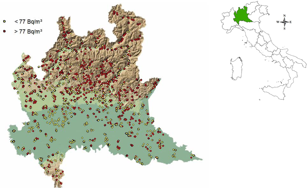
2. Experimental Section: The Data
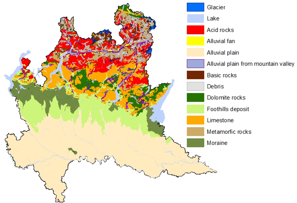
2.1. Geogenic Factors
- acid rocks: igneous and metamorphic rocks like rhiolite, granites, gneiss and orthogneisses
- basic rocks: igneous and metamorphic rocks like andesite, diorite, amphibolite and serpentinite
- metamorphic rocks: phyllite, schists and mica schists
- dolomite rocks
- limestone
- alluvial fan: fan-shaped deposits at the exit of main valley
- debris: landslides, rock falls and shallow debris flows, due to action of gravity.
- alluvial plain from mountain valley: deposits of fluvial rivers forming floodplains and terraces of river valleys, in the mountain area
- moraine: accumulation of unconsolidated glacial debris (soil and rock)
- foothill deposit: deposits of fluvial rivers, highly permeable, in the transition zone between plains and low relief hills to the adjacent topographically high mountains
- alluvial plain: deposits of fluvial rivers, low permeable, in the Po valley.
2.2. Building Factors
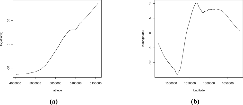
3. Methods
3.1. Kriging with External Drift
3.2. GLS Multiple Regression
- obtain a starting estimate of β, β̄0 that does not depend on θ (for example by OLS)
- compute the residuals r(s) = Z(s) – X (s) β̄
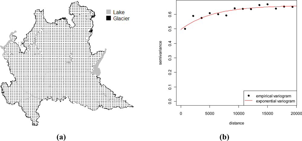
- estimate the variogram of the residuals, obtaining an estimate of θ, θ̄
- obtain a new estimate of β using Equation (5)
- Repeat steps 2–4 until the relative change in estimates of β and θ are small.
4. Results
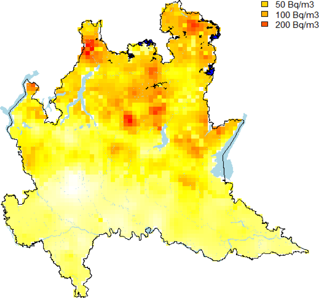
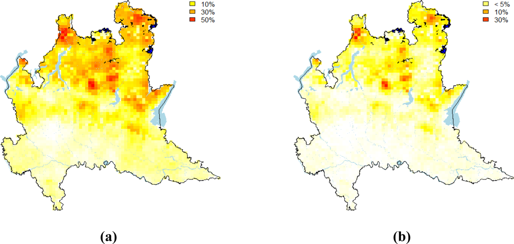
4.1. IRC Mapping
4.2. Assessing Anthropogenic and Geologic Influential Factors for IRC
5. Discussion and Conclusions
Acknowledgments
References and Notes
- International Agency for Research on Cancer (IARC). Man-made Mineral Fibres and Radon; WHO: Geneva, Switzerland, 1988. Available on line: http://monographs.iarc.fr/ENG/Monographs/vol43/volume43.pdf (accessed on 28 February 2011).
- Dubois, G; Bossew, P. A European Atlas of Natural Radiations Including Harmonized Radon Maps of the European Union. What Do We Have, What Do We Know, Quo Vadimus? Proceedings of the Terzo Convegno Nazionale Controllo ambientale degli agenti fisici: dal monitoraggio alle azioni di risanamento e bonifica, Biella, Italy, 7–9 June 2006.
- Nazaroff, WW; Nero, AV. Radon and Its Decay Products in Indoor Air; John Wiley & Sons: New York, NY, USA, 1988. [Google Scholar]
- Gates, AE; Gundersen, LCS. Geologic Controls on Radon; Geological Society of America: Washington, DC, USA, 1992; Special Paper 271. [Google Scholar]
- Zhu, HC; Charlet, JM; Tondeur, F. Geological controls to the indoor radon distribution in southern Belgium. Sci. Total Environ 1998, 220, 195–214. [Google Scholar]
- Ielsch, G; Cushing, ME; Combes, Ph; Cuney, M. Mapping of the geogenic radon potential in France to improve radon risk management: Methodology and first application to region Bourgogne. J. Environ. Radioact 2010, 101, 813–820. [Google Scholar]
- Chiles, JP; Delfiner, P. Geostatistics: Modeling Spatial Uncertainty; John Wiley & Sons: New York, NY, USA, 1999. [Google Scholar]
- Bertolo, A; Bigliotto, C; Giovani, C; Garavaglia, M; Spinella, M; Verdi, L; Pegoretti, S. Spatial distribution of indoor radon in Triveneto (northern Italy): A geostatistical approach. Radiat. Prot. Dosimetry 2009, 137, 318–323. [Google Scholar]
- Dubois, G; Bossew, P; Friedmann, H. A geostatistical autopsy of the Austrian indoor radon survey (1992–2002). Sci. Total Environ 2007, 377, 378–395. [Google Scholar]
- Franco-Marina, F; Villalba-Caloca, J; Segovia, N; Tavera, L. Spatial indoor radon distribution in Mexico City. Sci. Total Environ 2003, 317, 91–103. [Google Scholar]
- Zhu, HC; Charlet, JM; Poffijn, A. Radon risk mapping in southern Belgium: An application of geostatistical and GIS techniques. Sci. Total Environ 2001, 272, 203–210. [Google Scholar]
- Nero, AV; Schwehr, MB; Nazaroff, WW; Revzan, KL. Distribution of airborne radon-222 concentrations in US homes. Science 1986, 234, 992–997. [Google Scholar]
- Raspa, G; Salvi, F; Torri, G. Probability mapping of indoor radon-prone areas using disjunctive kriging. Radiat. Prot. Dosimetry 2010, 138, 3–19. [Google Scholar]
- Borgoni, R; Quatto, P; Somà, G; de Bartolo, D. A geostatistical approach to define guidelines for radon prone area identification. Stat. Methods Appl 2010, 19, 255–276. [Google Scholar]
- Apte, MG; Price, PN; Nero, AV; Revzan, KL. Predicting New Hampshire indoor radon concentrations from geologic information and other covariates. Environ. Geol 1999, 37, 181–194. [Google Scholar]
- Price, PN; Nero, AV; Gelman, A. Bayesian prediction of mean indoor radon concentrations for Minnesota counties. Health Phys 1996, 71, 922–936. [Google Scholar]
- Lévesque, B; Gauvin, D; McGregor, RG; Martel, R; Gingras, S; Dontigny, A; Walker, WB; Lajoie, P; Létourneau, E. Radon in residences: Influences of geological and housing characteristics. Health Phys 1997, 72, 907–914. [Google Scholar]
- Shi, X; Hoftiezer, DJ; Duell, EJ; Onega, TL. Spatial association between residential radon concentration and bedrock types in New Hampshire. Environ. Geol 2006, 51, 65–71. [Google Scholar]
- Smith, BJ; Field, RW. Effect of housing factor and surficial uranium on the spatial prediction of residential radon in Iowa. Environmetrics 2007, 18, 481–497. [Google Scholar]
- Gunby, JA; Darby, SC; Miles, JC; Green, BM; Cox, DR. Factors affecting indoor radon concentrations in the United Kingdom. Health Phys 1993, 64, 2–12. [Google Scholar]
- Sundal, AV; Henriksen, H; Soldal, O; Strand, T. The influence of geological factors on indoor radon concentrations in Norway. Sci. Total Environ 2004, 328, 41–53. [Google Scholar]
- Buchli, R; Burkart, W. Influence of subsoil geology and construction technique on indoor air 222Rn levels in 80 houses of the central Swiss Alps. Health Phys 1989, 56, 423–429. [Google Scholar]
- Tell, I; Bensryd, I; Rylander, L; Jönsson, G; Daniel, E. Geochemistry and ground permeability as determinants of indoor radon concentrations in southernmost Sweden. Appl. Geochem 1994, 9, 647–655. [Google Scholar]
- Borgoni, R. A quantile regression approach to evaluate factors influencing residential indoor radon concentration. Environ Model Assess 2011. [Google Scholar] [CrossRef]
- Cinelli, G; Tondeur, F; Dehandschutter, B. Development of an indoor radon risk map of the Walloon region of Belgium, integrating geological information. Environ. Earth Sci 2011, 62, 809–819. [Google Scholar]
- Kemski, J; Klingel, R; Siehl, A; Valdivia-Manchego, M. From radon hazard to risk prediction-based on geological maps, soil gas and indoor measurements in Germany. Environ. Geol 2009, 56, 1269–1279. [Google Scholar]
- Eurostat—European Commission Homepage. Available online: http://epp.eurostat.ec.europa.eu (accessed on 31 January 2011).
- Bochicchio, F; Campos Venuti, G; Nuccetelli, C; Piermattei, S; Risica, S; Tommasino, L; Torri, G. Results of the representative Italian national survey on radon indoors. Health Phys 1996, 71, 741–748. [Google Scholar]
- Sesana, L; Polla, G; Facchini, U; De Capitani, L. Radon-prone areas in the Lombard plain. J. Environ. Radioact 2005, 82, 51–62. [Google Scholar]
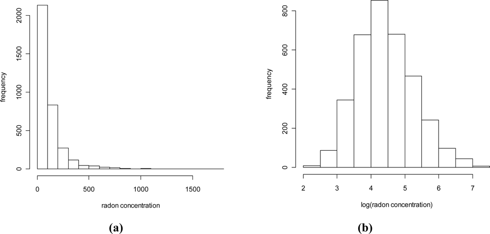
- Bossew, P. Radon: Exploring the log-normal mystery. J. Environ. Radioact 2010, 101, 826–834. [Google Scholar]
- Murphy, P; Organo, C. A comparative study of lognormal, gamma and beta modelling in radon mapping with recommendations regarding bias, sample sizes and the treatment of outliers. J. Radiol. Prot 2008, 28, 293–302. [Google Scholar]
- Tuia, D; Kanevski, M. Indoor radon distribution in Switzerland: Lognormality and extreme value theory. J Environ Radioact 2008, 99, 649–657. [Google Scholar]
- Hastie, TJ; Tibshirani, RJ. Generalized Additive Models; Chapman & Hall/CRC: New York, NY, USA, 1990. [Google Scholar]
- Appleton, JD; Miles, JCH. A statistical evaluation of the geogenic controls on indoor radon concentrations and radon risk. J. Environ. Radioact 2010, 101, 799–803. [Google Scholar]
- Bossew, P; Dubois, G; Tollefsen, T. Investigations on indoor Radon in Austria, part 2: Geological classes as categorical external drift for spatial modelling of the Radon potential. J. Environ. Radioact 2008, 99, 81–97. [Google Scholar]
- ARPA Piemonte. La Mappatura del Radon in Piemonte; ARPA Piemonte: Ivrea TO, Italy 2009. Available online: http://www.arpa.piemonte.it/upload/dl/Pubblicazioni/2009_-_La_mappatura_del_radon_in_Piemonte/La_mappatura_del_radon_in_Piemonte.pdf (accessed on 28 February 2011).
- Buttafuoco, G; Tallarico, A; Falcone, G. Mapping soil gas radon concentration: A comparative study of geostatistical methods. Environ. Monit. Assess 2007, 131, 135–151. [Google Scholar]
- Ciotoli, G; Etiope, G; Guerra, M; Lombardi, S. The detection of concealed faults in the Ofanto Basin using the correlation between soil-gas fracture surveys. Tectonophysics 1999, 301, 321–332. [Google Scholar]
- Infrastruttura per l’Informazione Territoriale della Lombardia. Geoportale della Lombardia. Available online: http://www.cartografia.regione.lombardia.it/geoportale (accessed on 2 February 2011).
- It was not possible to reconstruct the geological type for 12 points. These have been discarded from the analysis.
- Foxall, R; Baddeley, A. Nonparametric measures of association between a spatial point process and a random set, with geological applications. Appl. Statist 2002, 51, 165–182. [Google Scholar]
- Cressie, NAC. Statistics for Spatial Data; John Wiley & Sons: New York, NY, USA, 1993. [Google Scholar]
- Goovaerts, P. Geostatistics for Natural Resources Evaluation; Oxford University Press: New York, NY, USA, 1997. [Google Scholar]
- Schabenberger, O; Gotway, CA. Statistical Methods for Spatial Data Analysis; Chapman & Hall/CRC: New York, NY, USA, 2005. [Google Scholar]
- R Development Core Team, R: A Language and Environment for Statistical Computing; R Foundation for Statistical Computing: Vienna, Austria, 2010.
- De Boor, C. A Practical Guide to Splines; Springer-Verlag: New York, NY, USA, 2001. [Google Scholar]
- The model has been estimated using 3,248 measurements. 264 observations were discarded from the analysis because of missing values in the relevant covariates.
- The regression model for IRC has been estimated on a log scale. In the y-axis of Figure 10 the exponential transformation of the estimated expected values has been reported.


| Statistics | Value |
|---|---|
| No. of sites | 3,512 |
| Mean | 124 |
| Median | 77 |
| Standard deviation | 141 |
| Min | 9 |
| Max | 1,796 |
| Geological classes | No. of sites (%) | Mean Bq/m3 | Sd Bq/m3 | Median Bq/m3 | % above 200 Bq/m3 | % above 400 Bq/m3 |
|---|---|---|---|---|---|---|
| Alluvial plain | 833 (24%) | 66 | 50 | 53 | 2 | 0 |
| Foothill deposit | 667 (19%) | 118 | 115 | 76 | 15 | 3 |
| Limestone | 333 (10%) | 137 | 148 | 88 | 18 | 6 |
| Alluvial fan | 136 (4%) | 125 | 115 | 88 | 16 | 3 |
| Debris | 246 (7%) | 207 | 224 | 148 | 33 | 9 |
| Dolomite rocks | 246 (7%) | 198 | 197 | 127 | 30 | 13 |
| Acid rocks | 183 (5%) | 192 | 204 | 113 | 29 | 13 |
| Basic rocks | 32 (1%) | 83 | 82 | 59 | 6 | 3 |
| Metamorphic rocks | 174 (5%) | 148 | 125 | 111 | 22 | 3 |
| Alluvial plain from mountain valley | 213 (6%) | 168 | 169 | 117 | 28 | 8 |
| Moraine | 437 (12%) | 92 | 90 | 64 | 9 | 2 |
| Building characteristics | No. of sites (%) | Mean Bq/m3 | Sd Bq/m3 | Median Bq/m3 | % above 200 Bq/m3 | % above 400 Bq/m3 |
|---|---|---|---|---|---|---|
| Type of building | ||||||
| Single | 2,364 (67%) | 131 | 140 | 84 | 18 | 5 |
| Non single | 1,073 (31%) | 107 | 136 | 68 | 10 | 3 |
| Missing value | 75 (2%) | |||||
| Type of soil connection | ||||||
| Contact with ground | 1,259 (36%) | 146 | 156 | 91 | 21 | 7 |
| Basement/Crawl space | 2,116 (60%) | 111 | 130 | 71 | 12 | 3 |
| Missing value | 137 (4%) | |||||
| Wall material | ||||||
| Stone | 511 (15%) | 161 | 186 | 104 | 24 | 7 |
| Other materials | 2,946 (84%) | 118 | 131 | 74 | 14 | 4 |
| Missing value | 55 (1%) | |||||
| Geological Classes | No. of grid points |
|---|---|
| Alluvial plain | 1,030 |
| Foothill deposit | 316 |
| Limestone | 212 |
| Alluvial fan | 8 |
| Debris | 102 |
| Dolomite rocks | 175 |
| Acid rocks | 233 |
| Basic rocks | 38 |
| Metamorphic rocks | 180 |
| Alluvial plain from mountain valley | 33 |
| Moraine | 188 |
| Coefficients | Standard error | t-value | p-value | |
|---|---|---|---|---|
| Intercept | 4,004 | 0,101 | 39,834 | <0,0001 |
| Foothill deposit | 0,357 | 0,074 | 4,819 | <0,0001 |
| Limestone | 0,355 | 0,092 | 3,875 | 0,0001 |
| Alluvial fan | 0,412 | 0,116 | 3,559 | 0,0004 |
| Debris | 0,732 | 0,102 | 7,203 | <0,0001 |
| Dolomite rocks | 0,584 | 0,101 | 5,789 | <0,0001 |
| Acid Rocks | 0,592 | 0,110 | 5,388 | <0,0001 |
| Basic rocks | 0,066 | 0,178 | 0,372 | 0,7102 |
| Metamorphic rocks | 0,575 | 0,113 | 5,105 | <0,0001 |
| Alluvial plain from mountain valley | 0,592 | 0,102 | 5,778 | <0,0001 |
| Moraine | 0,140 | 0,088 | 1,600 | 0,1096 |
| Single building | 0,110 | 0,030 | 3,704 | 0,0002 |
| Contact with ground | 0,189 | 0,029 | 6,494 | <0,0001 |
| Stone wall material | 0,167 | 0,040 | 4,218 | <0,0001 |
© 2011 by the authors; licensee MDPI, Basel, Switzerland. This article is an open-access article distributed under the terms and conditions of the Creative Commons Attribution license (http://creativecommons.org/licenses/by/3.0/).
Share and Cite
Borgoni, R.; Tritto, V.; Bigliotto, C.; De Bartolo, D. A Geostatistical Approach to Assess the Spatial Association between Indoor Radon Concentration, Geological Features and Building Characteristics: The Case of Lombardy, Northern Italy. Int. J. Environ. Res. Public Health 2011, 8, 1420-1440. https://doi.org/10.3390/ijerph8051420
Borgoni R, Tritto V, Bigliotto C, De Bartolo D. A Geostatistical Approach to Assess the Spatial Association between Indoor Radon Concentration, Geological Features and Building Characteristics: The Case of Lombardy, Northern Italy. International Journal of Environmental Research and Public Health. 2011; 8(5):1420-1440. https://doi.org/10.3390/ijerph8051420
Chicago/Turabian StyleBorgoni, Riccardo, Valeria Tritto, Carlo Bigliotto, and Daniela De Bartolo. 2011. "A Geostatistical Approach to Assess the Spatial Association between Indoor Radon Concentration, Geological Features and Building Characteristics: The Case of Lombardy, Northern Italy" International Journal of Environmental Research and Public Health 8, no. 5: 1420-1440. https://doi.org/10.3390/ijerph8051420