Multi-Objective Aerodynamic and Structural Optimization of Horizontal-Axis Wind Turbine Blades

Abstract

A procedure based on MATLAB combined with ANSYS is presented and utilized for the multi-objective aerodynamic and structural optimization of horizontal-axis wind turbine (HAWT) blades. In order to minimize the cost of energy (COE) and improve the overall performance of the blades, materials of carbon fiber reinforced plastic (CFRP) combined with glass fiber reinforced plastic (GFRP) are applied. The maximum annual energy production (AEP), the minimum blade mass and the minimum blade cost are taken as three objectives. Main aerodynamic and structural characteristics of the blades are employed as design variables. Various design requirements including strain, deflection, vibration and buckling limits are taken into account as constraints. To evaluate the aerodynamic performances and the structural behaviors, the blade element momentum (BEM) theory and the finite element method (FEM) are applied in the procedure. Moreover, the non-dominated sorting genetic algorithm (NSGA) II, which constitutes the core of the procedure, is adapted for the multi-objective optimization of the blades. To prove the efficiency and reliability of the procedure, a commercial 1.5 MW HAWT blade is used as a case study, and a set of trade-off solutions is obtained. Compared with the original scheme, the optimization results show great improvements for the overall performance of the blade.

1. Introduction

With the world’s ever-increasing energy demands in the presence of continuous fossil fuel shortage and environmental pollution, various renewable energy sources are currently being investigated [1,2,3,4]. Wind energy has been widely accepted because of its great advantages, such as inexhaustibility and environmental friendliness [5,6]. Vigorous development and utilization of wind energy is of great significance to improving energy structure and achieving sustainable development. A typical arrangement to extract wind energy is the use of wind turbines, especially the horizontal-axis wind turbine (HAWT), which is the most valuable and widely used form at present [7]. In order to make wind energy more competitive with other energy sources, the wind turbines are designed aiming at minimizing the cost of energy (COE), namely, increasing the annual energy production (AEP) and bringing down the total cost.

Blade is the key component of wind turbine to capture wind energy, it is of course not excluded from the overall optimization goals. The blade design process mainly includes two stages: the aerodynamic design and the structural design. The two stages are separated by the conventional methods to simplify the process, and the aerodynamic design is paid more attention to. However, with the growth in turbine size and blade length, multi-megawatt (MW) sized blades are now requiring designers to consider the structure of the blade earlier in the design process [8].

Modern blades are primarily made of glass fiber reinforced plastic (GFRP) due to its low density and superior mechanical properties. As the blade length increases, there is a rapid growth in the blade mass (approximately as a cubic power of length, while the trend of many modern blades has maintained 2.3 power [8]) as well as the loads. Even GFRP cannot satisfy the structural requirements, which leads to the employment of lighter and stronger materials such as carbon fiber reinforced plastic (CFRP) [9]. Since CFRP is much more expensive than GFRP, the obvious disadvantage is increased cost, but it will be mitigated somewhat by a reduction in blade mass. Therefore, it is an important issue to arrange the GFRP and CFRP in a sufficient way to reach the optimal utilization of the material. Many researches [9,10,11,12,13] have recently been carried out to deal with such problems using numerical methods or optimization techniques, the results showed improvements in structural behaviors of the blades, but the aerodynamic performances were not considered.

A successful blade design must integrate both aerodynamic and structural concerns to get the overall optimal solutions. However, only a limited number of papers [2,14,15,16,17,18] are focused on the optimization for this purpose. Most of the works among these papers either taken a single objective function in the problem or used beam models to calculate the structural behaviors, the material layup was not discussed. Our recent research [19] described a multi-objective optimization method for the aerodynamic and structural integrated design of blades to maximize the AEP and minimize the blade mass, finite element method (FEM) was applied so that the layup variation could be described, but the cost was not evaluated due to no CFRP usage.

This paper presents a procedure for the multi-objective aerodynamic and structural optimization of HAWT blades based on the one in [19]. The blade element momentum (BEM) theory is used to evaluate the aerodynamic performances, the FEM method is applied to calculate the structural behaviors. Moreover, the non-dominated sorting genetic algorithm (NSGA) II is adapted for the multi-objective optimization of the blades. Materials of CFRP combined with GFRP are used in the spar cap, and a material cost function is added in the procedure. The goal is to find a balance between the aerodynamic design and structural design to minimize the COE of HAWT blades.

2. Modeling of the Blade

2.1. Geometry Shape and Aerodynamic Loads

The geometry shape of a typical HAWT blade is shown in Figure 1, which generally includes three regions: the root region normally with circular cross-section, the aerodynamic region with thinner airfoils to capture wind energy and the region transition from the root to the airfoil section at 15% radius with a high thickness to chord ratio of up to about 50%. The three parts consist of the airfoil series and their locations, the chord and twist distributions.

In order to define the blade geometry shape, seven control points (CPs) with fixed locations are applied for the chord and twist distributions, as shown in Figure 2. CP1 is at root, CP3 is at the maximum chord station and CP7 is at tip. The chord of CP2 is equal to CP1, and the twists of CP1–3 are the same. The airfoil locations are reflected by the percent thickness distribution, as illustrated in Figure 3. Six more CPs, which represent the airfoil locations and percent thicknesses, are used for the percent thickness distribution. Then, the chord, twist and percent thickness are defined with B-Spline curves.

Once the geometry shape of the blade is fixed, the aerodynamic loads can be calculated using BEM theory [20,21] by dividing the blade into several independent elements. Aerodynamic loads including operational case and ultimate case for the optimization design in this paper are the same as the loads in [19]. The operational case takes into account the maximum root flap bending moment M_flap under operational state, which is computed as follow:

$$M_{flap}={\displaystyle {\int }_0^{R}4\mathsf{\pi }\mathsf{\rho }{u}^{2}a}(1-a)F{r}^{2}dr$$

(1)

where $\mathsf{\rho }$ is the air density, u is the wind speed, a is the axial induction factor, F is the Prandtl’s tip and root correction factor, and R is the blade length.

The maximum bending moment can be derived from dividing the range of wind speeds into different values every 0.5 m/s, and the corresponding wind speed u can be determined. Therefore, the lift force L and drag force D per unit length can be calculated as follow:

$$\{\begin{array}{l}L=\frac{1}{2}\mathsf{\rho }{W}^{2}c\left(r\right)C_l\\ D=\frac{1}{2}\mathsf{\rho }{W}^{2}c\left(r\right)C_d\end{array}$$

(2)

where W is a relative velocity related to u, c(r) is the local chord, C_l and C_d are the lift and drag coefficients.

Then, the lift and drag forces are projected into normal to and tangential to the rotor plane directions to obtain the forces dp_N and dp_T, as show in Equation (3):

$$\{\begin{array}{l}d{p}_N=dLcos\mathsf{\varphi }+dDsin\mathsf{\varphi }=\frac{1}{2}\mathsf{\rho }{W}^{2}c\left(r\right)(C_{l}cos\mathsf{\varphi }+C_{d}sin\mathsf{\varphi })dr\\ d{p}_T=dLsin\mathsf{\varphi }-dDcos\mathsf{\varphi }=\frac{1}{2}\mathsf{\rho }{W}^{2}c\left(r\right)(C_{l}sin\mathsf{\varphi }-C_{d}cos\mathsf{\varphi })dr\end{array}$$

(3)

where dp_N is the force normal to the rotor plane, dp_T is the force tangential to the rotor plane, ϕ is the angle between the rotor plane and the relative velocity, as shown in Figure 4.

The ultimate case is derived from the parked 50 year extreme wind condition, which can be calculated approximately by empirical formula [22]:

$$p(r)=\frac{1}{2}\mathsf{\rho }{C}_f{V}_b^2{k}_t^2{\left[ln\left(\frac{h_{hub}+2/3R}{z_0}\right)+3\right]}^{2}c(r)$$

(4)

where $C_f$ is a force coefficient, $V_b$ is a basis wind speed, $k_t$ is a terrain factor, $h_{hub}$ is the hub height and $z_0$ is a roughness length. If the surrounding of a wind farm has no nearby obstacles and very low vegetation, $k_t=0.17$ and $z_0=0.01\mathrm{m}$.

2.2. Structural form and Finite Element Method Model of the Blade

Figure 5 shows a typical structural form of the blade cross section, which can be divided into four parts: leading edge, spar cap, shear webs and trailing edge. The spar cap mainly consists of unidirectional laminates such as GFRP or CFRP, while the leading edge, shear webs and trailing edge consist of sandwich structure materials. Material properties of the unidirectional laminates are shown in

Table 1. Material properties of the unidirectional laminates. GFRP: glass fiber reinforced plastic; and CFRP: carbon fiber reinforced plastic.

Material	E1 (GPa)	E2 (GPa)	G12 (GPa)	v12	$\mathsf{\rho }$ (kg/m3)	Cost (m−3)
GFRP	42.19	12.53	3.52	0.24	1910	1
CFRP	130.00	10.30	7.17	0.28	1540	10

, the cost of CFRP is set as 10 times than that of GFRP [12]. Usually the spar cap provides the stiffness and strength requirements of the blade, its thickness in the middle of the blade is typically large in comparison to those of other parts. Consequently, the spar cap makes a major contribution to the blade mass and cost [23], which should be paid more attention to during the optimization process.

The FEM modeling process of the blade is complicated and time-consuming, in order to simplify and expedite the creation and analysis the models, including parametric design studies to create various models, the ANSYS parametric design language (APDL) in ANSYS software (Version 14.0, ANSYS Inc., Canonsburg, PA, USA) is applied. After inputting the geometry shape, the structure of the blade is modeled with shell elements (SHELL99 element type for the spar cap and SHELL91 element type for the other three parts). The two types of elements are capable of representing layer characteristics by defining the real constants, namely, the material properties, orientations and thicknesses. Appropriate number of real constants should be determined in order to find a balance between accuracy and computation cost. Moreover, a mapping meshing method is applied to prevent erroneous results.

3. Optimization Model

3.1. Design Variables

Once the airfoil series and the blade length are confirmed, the geometrical shape contributes directly to the aerodynamic performances. Therefore, the chords, twists and airfoil locations of the CPs in Figure 2 and Figure 3 are selected as aerodynamic variables. The root diameter is set not to change, which means the chords of CP1 and CP2 are fixed, so five aerodynamic variables (x₁ to x₅) are used for the chords of CP3–7. As the twist remains constant inboard of the maximum chord, another five aerodynamic variables (x₆ to x₁₀) are employed for the twist of CP3–7. The location of CP8 is at root and the location of CP13 is at tip, thus four more aerodynamic variables (x₁₁ to x₁₄) are needed for the locations of CP9–12 (airfoils with percent thickness of 40%, 30%, 25% and 18%). Furthermore, the rated rotational speed of the rotor also has a great influence on the aerodynamic performances, thus it is selected as the last aerodynamic variable (x₁₅).

A typical material layup in the spar cap of commercial blade is shown in Figure 6. As mentioned earlier, the middle region (shown in green) of the spar cap contributes most to the blade mass and cost. Hence, the material layup in this region and its width are selected as structural variables. Eight discrete CPs with different number and location of layers are used to simulate the layup, as shown in Figure 7. CP16–19 each has three variables that are the number of GFRP layers, the number of CFRP layers and the location of layers, while the other four points each has two variables that are the number of GFRP layers and the number of CFRP layers. In addition, the number of layers of CP17–18 are defined the same. Therefore, eighteen structural variables are used for the material layup, x₁₆ to x₂₂ for the number of GFRP layers, x₂₃ to x₂₉ for the number of CFRP layers and x₃₀ to x₃₃ for the location of layers. Another variable x₃₄ is used for the width of the spar cap. In addition, the blade mass and cost can further decrease if the shear webs are positioned appropriately, so the position of the shear webs is selected as the last structural variable (x₃₅).

3.2. Objective Functions

The purpose of the present work is to minimize the COE of the blade, namely, increasing the AEP and reducing the cost. In addition, the blade mass is another important goal for blade design. The reduction in blade mass could not only reduce the cost but also the loads, which has a multiplier effect throughout the system including the foundation [24]. Therefore, an AEP function, a mass function and a material cost function are taken into account as the three objectives of the problem. In order to enable visual comparisons between the optimization results and original values, dimensionless method is applied to the functions.

The first objective function is computed by normalizing the current AEP to the value of the original blade $AE{P}_0$, which is defined as:

$$f\left(1\right)=max(AEP/AE{P}_0)$$

(5)

$$AEP={\displaystyle \sum _{i=1}^N\frac{1}{2}}[P(u_i)+P(u_{i+1})]\times f(u_i<u_0<u_{i+1})\times 8760$$

(6)

$$P(u_i)={\displaystyle {\int }_0^{R}4\mathsf{\pi }{r}^3\mathsf{\rho }{u}_i{\mathsf{\omega }}^2{a}^{\prime }(1-a)Fdr}$$

(7)

$$f(u_i<u_0<u_{i+1})=exp\left(-{\left(\frac{u_i}{A}\right)}^k\right)-exp\left(-{\left(\frac{u_{i+1}}{A}\right)}^k\right)$$

(8)

where $P\left(u_i\right)$ is the power of the wind turbine, $f(u_i<u_0<u_{i+1})$ is the probability of wind speed occurrence determined by the Weibull probability distribution curve, $\mathsf{\omega }$ is the rotational speed of the blade, $a^{\prime }$ is the tangential induction factor, $k$ is a form factor, and $A$ is a scaling factor.

The second objective function is the ratio between the mass of the current blade and the original blade $mas{s}_0$, expressed as:

$$f\left(2\right)=min(mass/mas{s}_0)$$

(9)

$$mass={\displaystyle \sum _i{\mathsf{\rho }}_i\times V_i}$$

(10)

where ${\mathsf{\rho }}_i$ is the material density, $V_i$ is the volume of the material.

The third objective function is comprised of the cost of the current blade dividing the original value $cos{t}_0$, as shown in the following Equations:

$$f\left(3\right)=min(cost/cos{t}_0)$$

(11)

$$cost={\displaystyle \sum _{j=1}^2{\displaystyle \sum _{i=1}^7(L{N}_i^j+L{N}_{i+1}^j)}}(L{L}_{i+1}^j-L{L}_i^j)\times SW\times C^j+C_c$$

(12)

where LN and LL are the number of layers and the locations of layers of the CPs, SW is the width of the spar cap, C is the material cost per cubic meter, C_c is the cost of the other parts of the blade, $j=1$ represents the usage of GFRP while $j=2$ represents the usage of CFRP.

3.3. Constraints

During the blade design process, lots of constraints such as aerodynamic and structural requirements should be well satisfied. In this paper, the constraints are: (1) geometrical shape [19]: the twist, chord and percent thickness distributions are required to monotonically decrease; (2) material layup: the number of layers shown in Figure 7 need to increase to a maximum value and then decrease, the location of layers need to monotonically increase; (3) maximum strain [25]: to meet the strength requirement, the maximum strains of GFRP ${\mathsf{\epsilon }}_{maxG}$ and CFRP ${\mathsf{\epsilon }}_{maxC}$ can not exceed the allowable values ${\mathsf{\epsilon }}_{dG}$ and ${\mathsf{\epsilon }}_{dC}$, respectively; (4) maximum tip deflection [26]: to avoid the risk of blade and tower collision, the maximum tip deflection d_max must be limited to a design value d_d; (5) natural frequency [27]: to prevent resonance, the first natural frequency of the blade F_blade−1 should be separated from the integral multiple of the rotor rotation frequency F_rotor; (6) buckling load [28]: the lowest buckling eigenvalue λ₁ is required to be larger than a safety factor to avoid buckling failure.

4. Description of the Optimization Procedure

In order to improve the overall performances of HAWT blades, a new optimization procedure with three modules is developed based on the one in [19]. Figure 8 shows the flowchart of the procedure.

First of all, an initial population including aerodynamic and structural variables is generated randomly between the proposed upper and lower bounds after inputting the basic parameters. The variables should also satisfy the constraints (1) and (2) mentioned in Section 3.3. Then, the aerodynamic analysis model handles the aerodynamic variables to define the geometry shape of the blade and evaluate the aerodynamic performances using BEM theory. Meanwhile, the structural analysis model deals with the structural variables to create a parametric FEM model of the blade by using APDL language in ANSYS and simulates the load cases to calculate the structural behaviors. In the next step, the three objective functions mentioned earlier are evaluated when several constraints have been checked. If the constraints are not satisfied, the population is neglected and the fitness functions will be set as infinite, which could guarantee the random generation of population feasible. Afterwards, the multi-objective optimization module is implemented to classify the solutions with NSGA II [29,30,31]. Finally, a new population will be created to restart the procedure until the optimization process converges (the iteration number reaches the maximum number of generations or the number of stall generations exceeds a default value), thus the Pareto optimal front can be obtained.

5. Application of the Procedure

5.1. Case Study

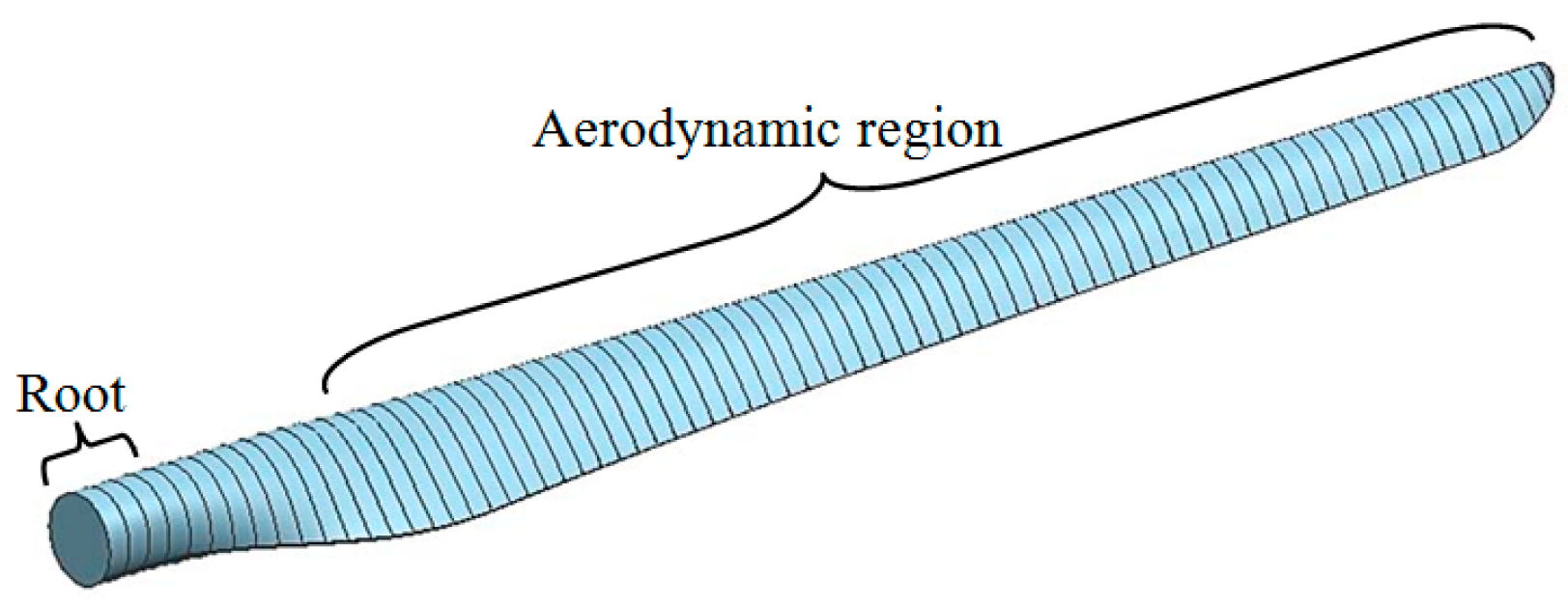
A commercial 1.5 MW fixed speed/variable pitch turbine blade with a length of 37 m is applied as a case study. The main geometrical features of the blade are summarized in

Table 2. The main geometrical features of the commercial 1.5 MW blade.

Location (m)	Airfoil	Chord (m)	Twist (°)	Percent Thickness (%)
0–1.0	Circle	1.88	10.00	100
6.8	DU400EU	3.02	10.00	40
9.3	DU300EU	2.98	7.30	30
13.7	DU91_W2_250	2.51	4.35	25
29.8	NACA_64_618	1.68	−0.33	18
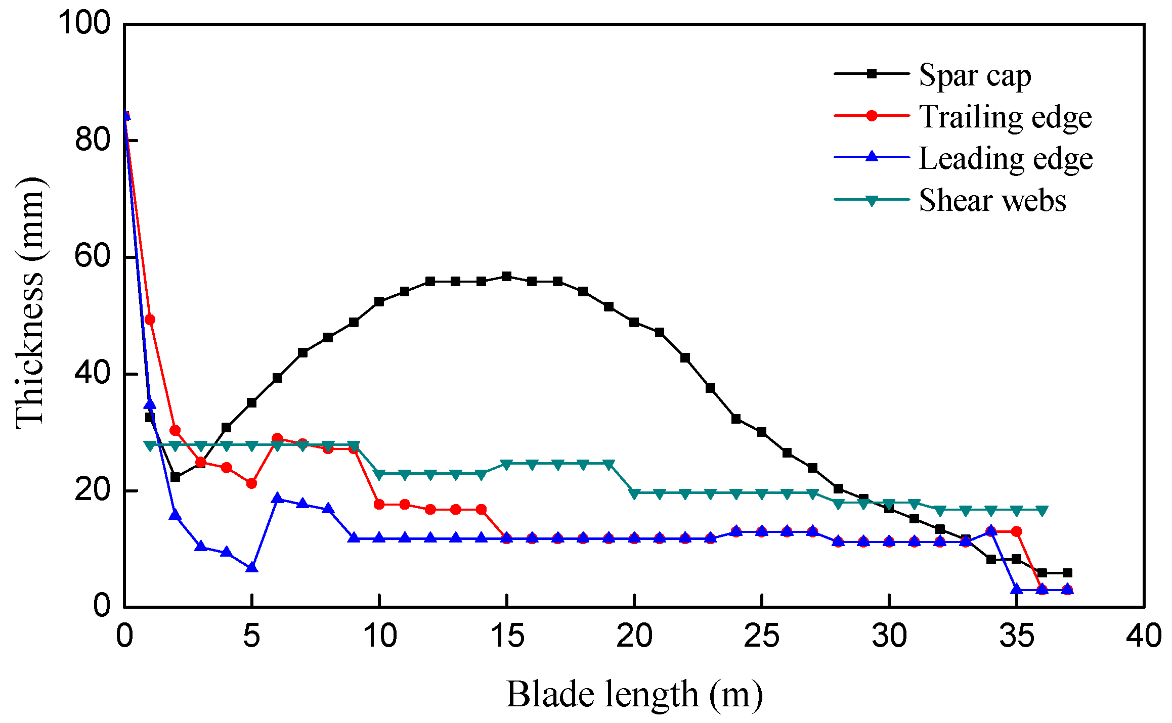
36.5	NACA_64_618	1.21	−1.13	18

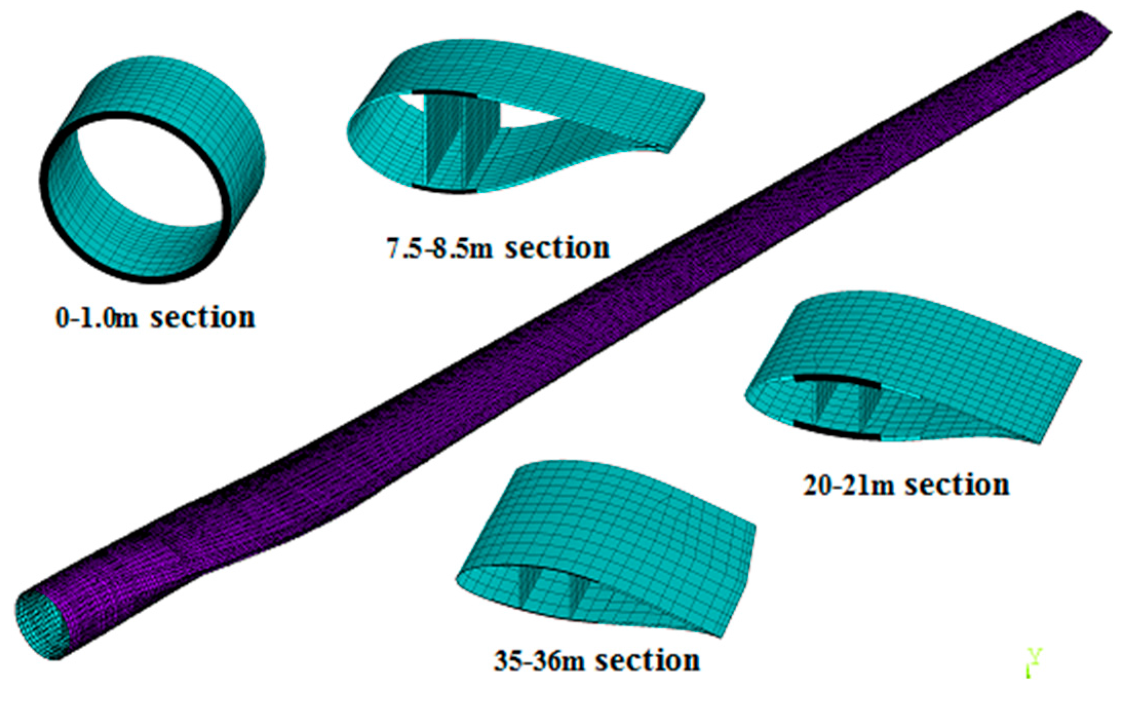
. As the tip region of the blade is mainly designed to reduce the aerodynamic noise caused by the blade interacts with the air flow, which contributes little to the structural performance, so the 0.5 m region at the tip is not considered in this research for convenience. The thickness distributions of the spar cap, leading edge, shear webs and trailing edge are shown in Figure 9. According to the thickness distributions, 290 real constants are defined through adjusting the model many times. The entire FEM model with a length of 36.5 m and some typical cross sections of the blade are shown in Figure 10. 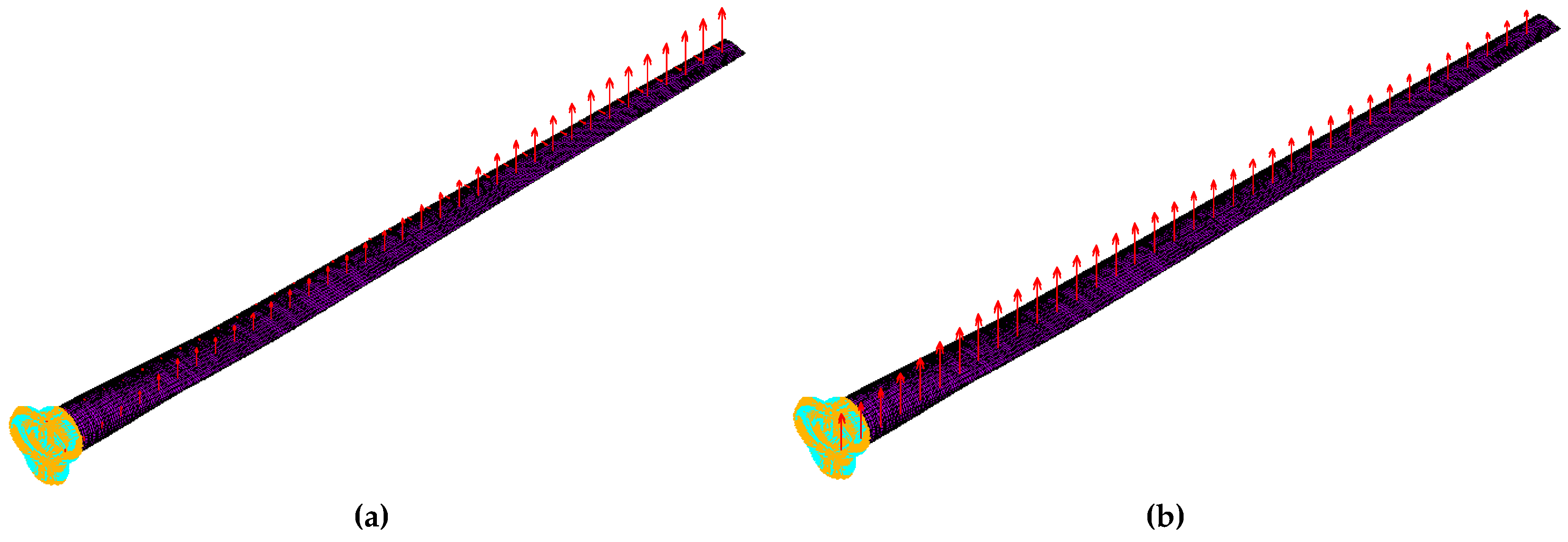Figure 11 shows the load distributions of the FEM model calculated in Section 2.1, the blade is divided into 36 cross sections every 1 m and the forces are applied on the cross sections as concentrated forces. The flap-wise, edge-wise and torsional rigidities validation process of the FEM model had been carried out in [19] to guarantee the reliability of the numerical simulation.

The basic parameters of the commercial 1.5 MW blade set in the procedure are listed in

Table 3. Basic parameters of the commercial 1.5 MW blade.

Parameter	Value	Unit
Rotor diameter	77	m
Number of blades	3	-
Hub diameter	3	m
Hub height	75	m
Rated wind speed	12	m/s
Rated rotational speed	19	rpm
Rated power	1500	kW
Cut-in wind speed	4	m/s
Cut-out wind speed	25	m/s
Air density	1.225	kg/m3

. The ranges of design variables and the constraint values are listed in

Table 4. Range of design variables and the constraint values.

Parameter	Min	Max	Unit
x1–x5	1.0	3.3	m
x6–x10	−2.0	12.0	°
x11–x14	6.0	30.0	m
x15	10	25	rpm
x16–x22	0	65	-
x23–x29	0	45	-
x30–x33	7.0	22.0	m
x34	0.50	0.70	m
x35	0.13	0.25	m
εdG	-	0.0050	-
εdC	-	0.0032	-
dd	-	5.5	m
λ1	1.2	-	-
Fblade-1	≤3Frotor − 0.3 or ≥3Frotor + 0.3		Hz

. The wind condition is derived from a local meteorological data of inland China with an annual average wind speed of 6 m/s, the turbulence parameter is 0.16, the values of Weibull form factor k and scaling factor A are calculated to be 1.91 and 6.8, respectively. The basic parameters of NSGA-II algorithm are: the population size is set as 80, the maximum number of generations is 50, and the probabilities of crossover and mutation are taken as 0.8 and 0.05, respectively.

5.2. Results and Discussion

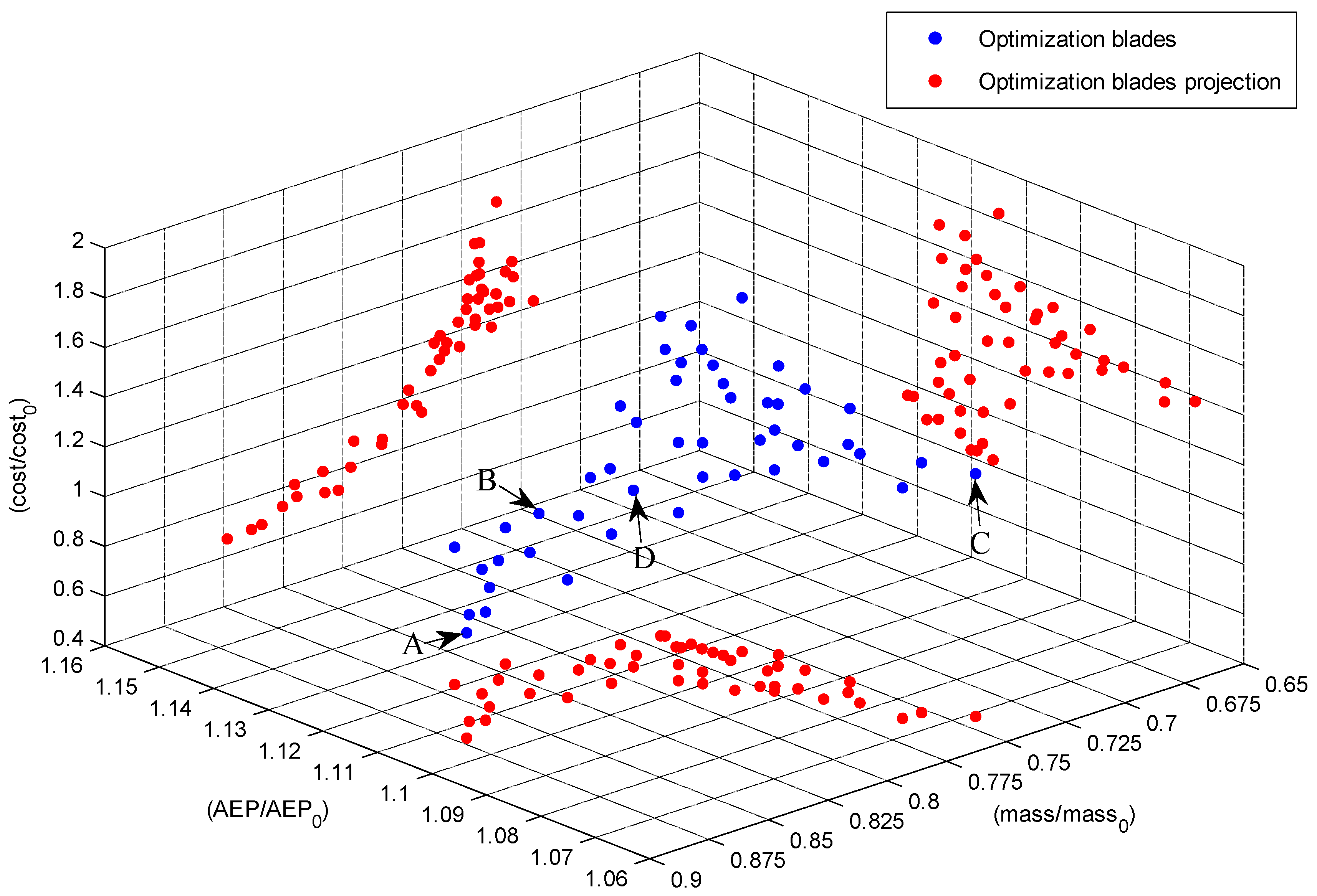
Figure 12 shows the final Pareto front of the airfoil-specific turbine blades derived from the procedure, it illustrates that an improvement on one objective will cause deteriorations on the other one or two objectives, which proves there are some conflicts between the selected objectives. The designer could chose the appropriate design based on specific goals and intentions. The projection of cost and mass reveals the relation of these two objectives is approximately monotonic. The same relation can also be found in the AEP and mass related Pareto front projection, while the relation of cost and AEP is rather complex. The extreme point design for each objective function (marked with A, B and C) and a design in the middle of the compromise region (marked with D) have been investigated further to show the properties of the design that lead to improved performances. Blade A has the lowest cost, blade B has the maximum AEP, and the mass of blade C is the lightest.

Table 5. Values of the design variables and objectives.

Parameter	Original Blade	Blade A	Blade B	Blade C	Blade D	Unit
x1	3.08	2.72	2.88	2.70	2.74	m
x2	2.88	2.51	2.63	2.50	2.51	m
x3	2.30	2.05	2.16	2.03	2.07	m
x4	1.82	1.62	1.70	1.61	1.63	m
x5	1.21	1.12	1.18	1.12	1.13	m
x6	10.00	10.15	10.60	10.21	10.24	°
x7	6.64	7.56	8.02	7.65	7.62	°
x8	3.14	4.10	4.53	4.04	4.12	°
x9	0.43	1.33	1.62	1.41	1.35	°
x10	−1.13	−0.49	−0.32	0.40	−0.45	°
x11	6.75	7.23	7.55	7.28	7.20	m
x12	9.50	9.95	10.33	10.20	9.89	m
x13	14.20	13.81	13.68	13.75	13.83	m
x14	28.95	26.62	25.53	26.73	26.36	m
x15	19.0	15.5	16.0	14.9	15.5	rpm
x16	33	30	24	9	20	-
x17	43	35	28	10	23	-
x18	53	45	35	11	28	-
x19	62	50	37	12	29	-
x20	53	39	31	11	21	-
x21	43	32	26	11	17	-
x22	33	29	17	9	13	-
x23	33	0	2	11	5	-
x24	43	0	3	15	7	-
x25	53	0	5	22	12	-
x26	62	0	7	25	13	-
x27	53	0	4	18	11	-
x28	43	0	3	18	9	-
x29	33	0	2	8	6	-
x30	7.8	8.1	8.3	8.1	8.3	m
x31	11.0	11.9	11.6	11.2	11.4	m
x32	18.0	17.8	17.3	17.1	17.5	m
x33	21.4	21.2	21.3	21.0	21.1	m
x34	0.620	0.56	0.59	0.55	0.56	m
x35	0.188	0.196	0.214	0.201	0.199	m
AEP	1.000	1.106	1.121	1.069	1.110	-
Mass	1.000	0.864	0.843	0.742	0.792	-
Cost	1.000	0.823	0.953	1.376	1.109	-

shows the design variable values and objective values of the original blade and the analyzed four blades.

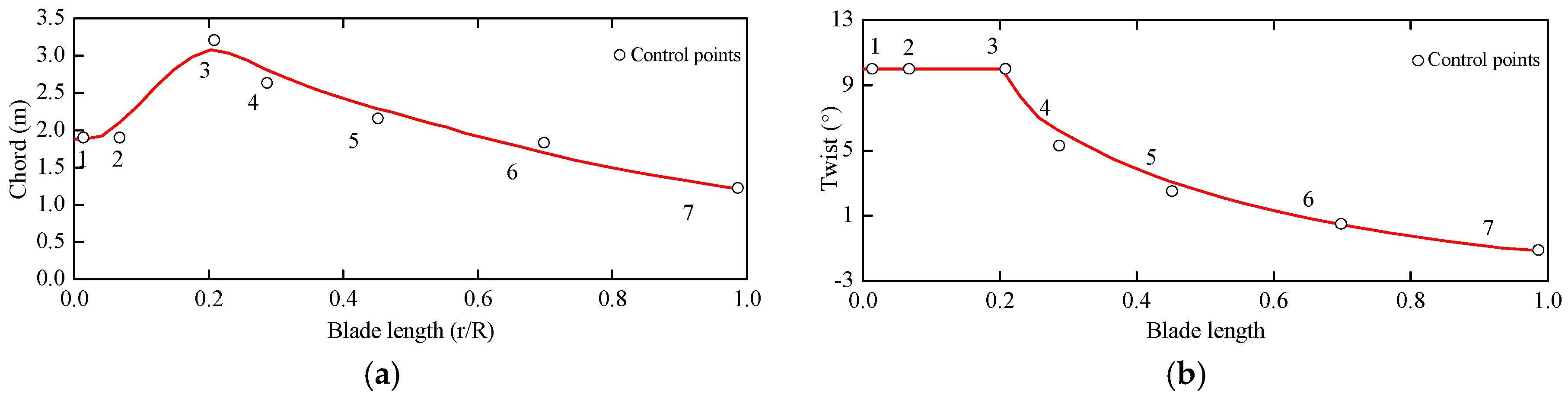
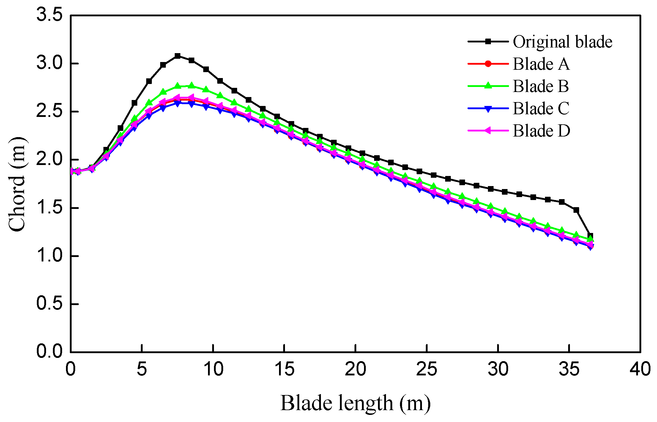
Figure 13 shows the chord distributions of the original and optimized blades. It can be seen that the chords all decrease after optimization, especially in the maximum chord region and the region close to the tip. As the root diameter is fixed, the chords of the optimized blades change slightly near the root. Although the decrease of chord would cause the power reduction in some degree, it can reduce the amount of materials and the thrust at the same time, which will lead to a lighter and cheaper blade. Because B-Spline curve is used for the chord distribution, the tip shape seems blunt compared with the original blade. However, as the 0.5 m region at the tip is not considered, the chords in this region could be adjusted and modified in the follow-up design process.

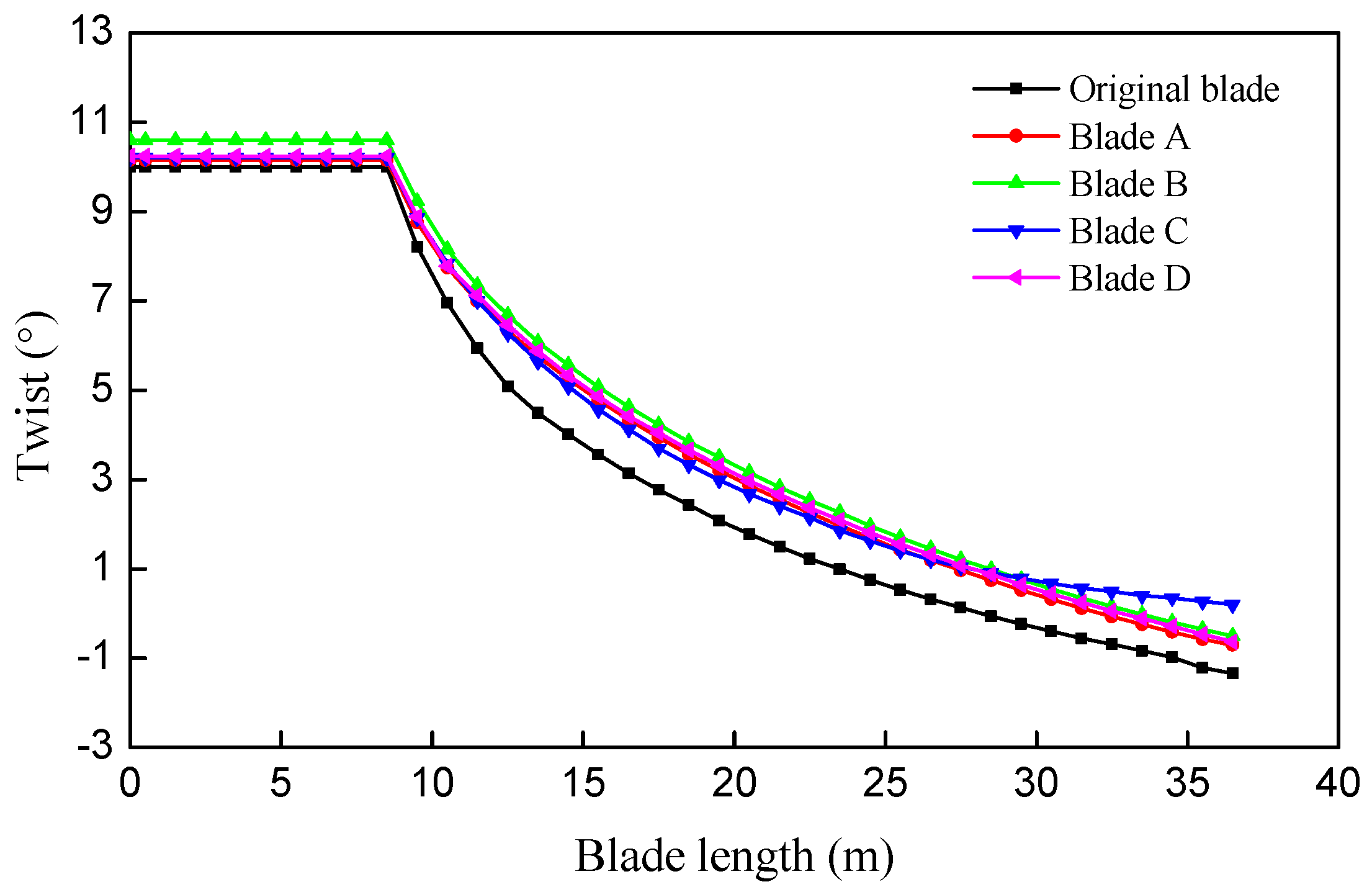
Figure 14 shows the twist distributions of the five blades. Because the root and the region near it are mainly design for structural reasons and contribute little to the aerodynamic performances, the twists in these regions are almost unchanged. In the aerodynamic region, the twists all increase after optimization, but the distribution trends almost remain the same with the original blade. The increase of the twists can result in a power increase to some extent, which is just the opposite of the chords reduction. This is because with the decreasing of the rotational speed (listed in Table 5), the angle between the mean relative velocity and tangential direction will increase. In order to maintain the high lift-to-drag ratios of the airfoils, the twists should also increase to keep the angle of attacks almost the same.

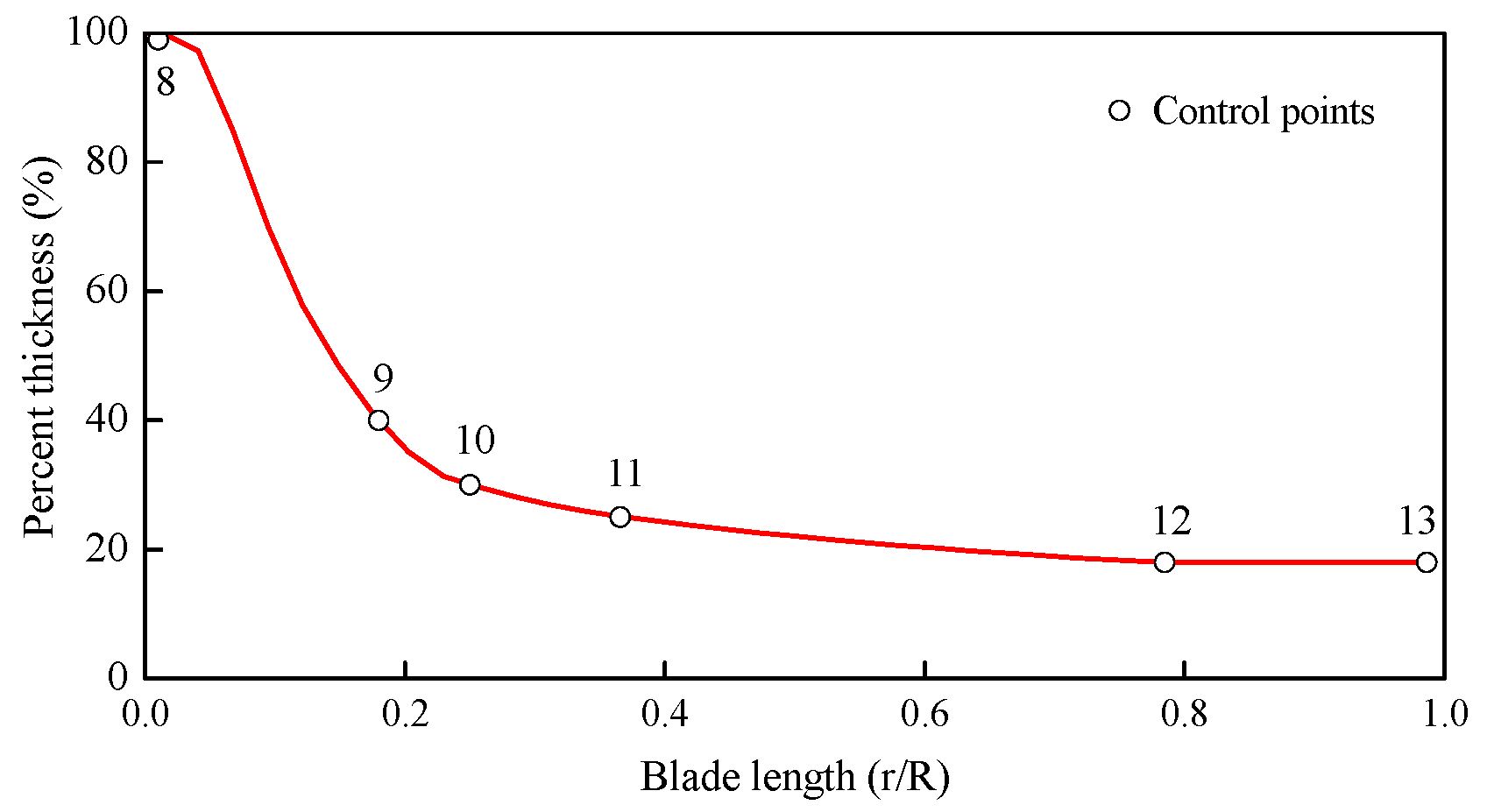
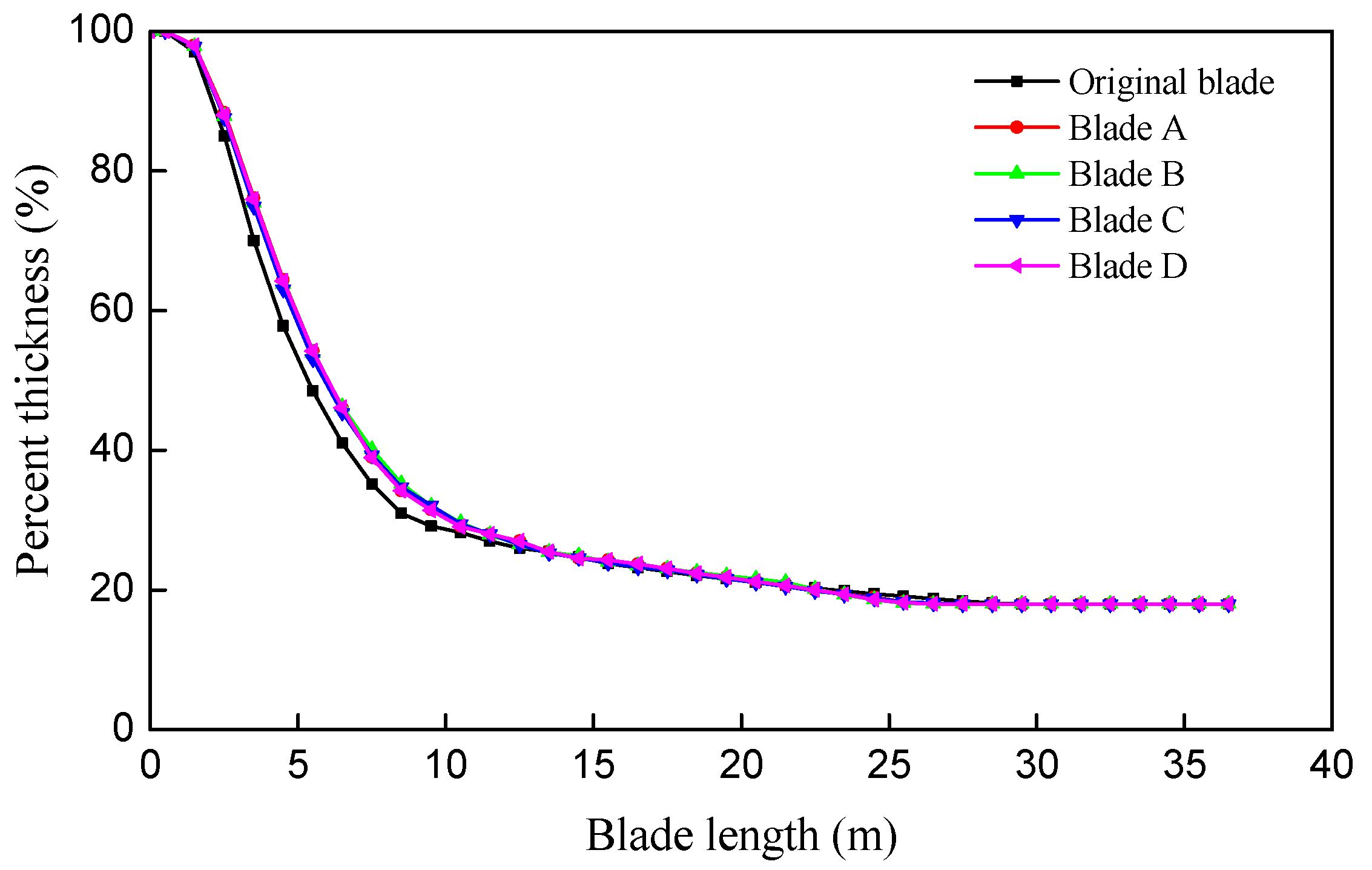
Figure 15 shows the percent thickness distributions of the five blades. The locations of the airfoils with 40% and 30% thicknesses increase (move toward the tip), while the locations of the airfoils with 25% and 18% thicknesses decrease (move toward the root) after optimization. The two thick airfoils move toward the tip means the percent thickness in the transition region increases, which would increase the section moment of inertia from the structural point of view. As the two thin airfoils have higher lift-to-drag ratios, moving their locations toward the root can increase the length of the main part that captures wind energy, which is beneficial to improve the power efficiency from the aerodynamic point of view.

To further find the blade designs with the improvements for the maximum AEP objective, the parallel coordinates in the design space is applied, as shown in Figure 16. The comparison reveals that: blade A and C exhibit a high correlation of aerodynamic variables, except for the twist at the tip and the rated rotational speed, which translates to larger twists above the original distribution trends in the main aerodynamic region and a smaller rotational speed for the design with lower AEP; blade D inherits most of the aerodynamic features from blade A but with a larger aerodynamic region and therefore a higher AEP; huge differences for most aerodynamic variables between blade B and blades A and C, which means larger chords, twists(with the same distribution trends of original design), the length of the main part that captures wind energy (approximately from the location of the 25% airfoil to the blade tip) and rotational speed are associated with higher AEP.

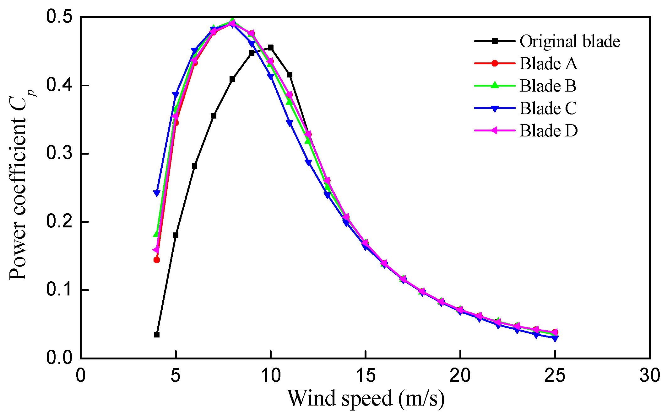
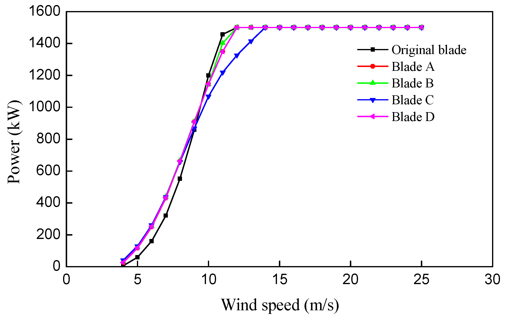
The comparison of power coefficients and powers between the five blades are shown in Figure 17 and Figure 18. Compared to the original blade, the power coefficients of the optimized blades increase significantly in the speed range of 4 to 9 m/s, then decrease slightly in the range of 10 to 13 m/s, and keep high values (exceed 0.4) in the range of 6 to 10 m/s. Each blade reaches the maximum power coefficient at 8 m/s wind speed, the maximum values all exceed 0.49, increased by more than 7.7% compared to the original blade. The rated wind speeds of the four optimized blades gradually increase from 12 to 14 m/s with the reduction of chords and rotational speed and the increase of twists, as shown in Figure 18. The comparisons in Figure 17 and Figure 18 show that the aerodynamic performances of the optimized blades are significantly improved at low wind speeds and drop a little when the wind speed increases. As the wind condition set in the procedure has much higher probabilities at low wind speeds, so the optimized blades can utilize more wind energy resources and thus to increase the AEP.

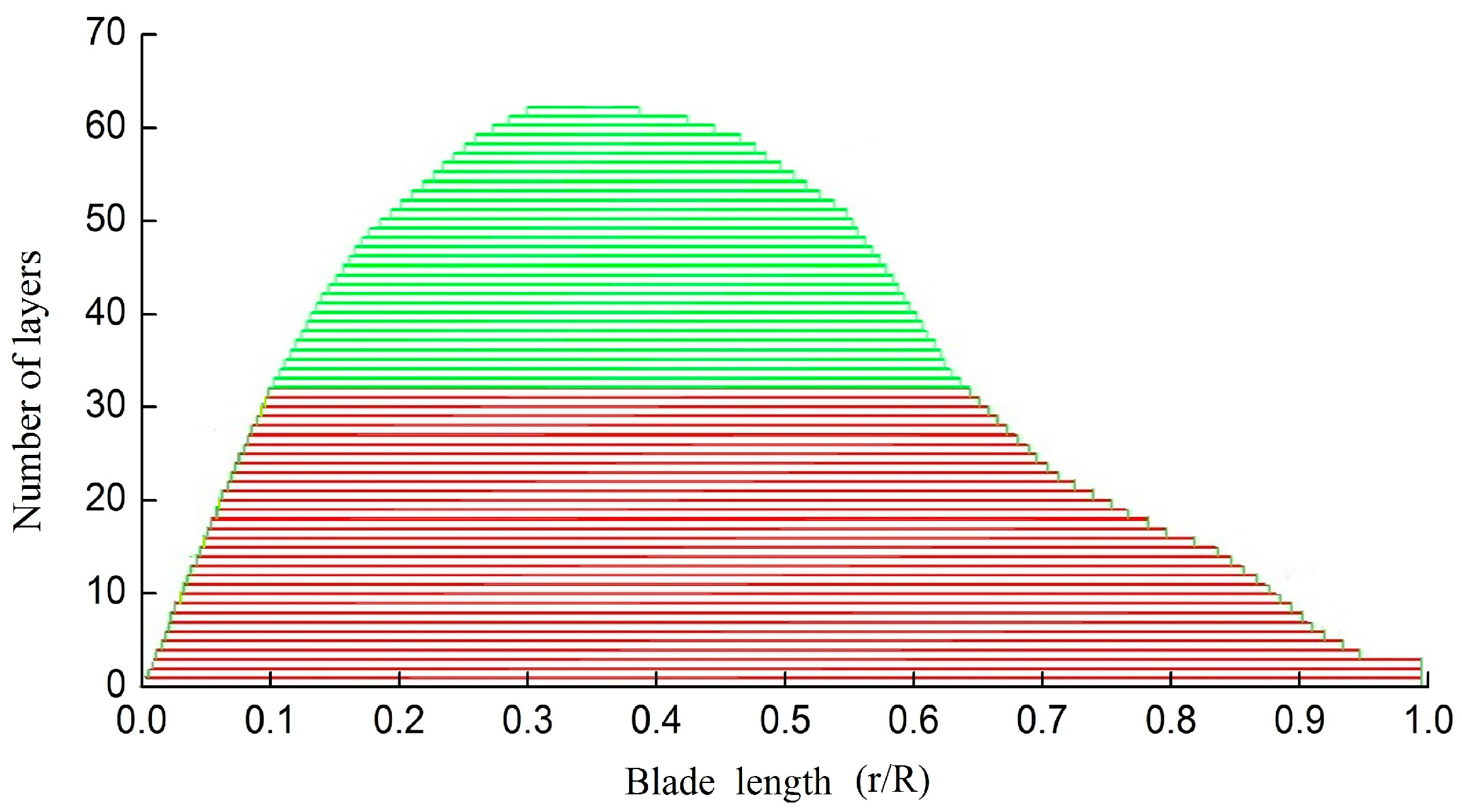
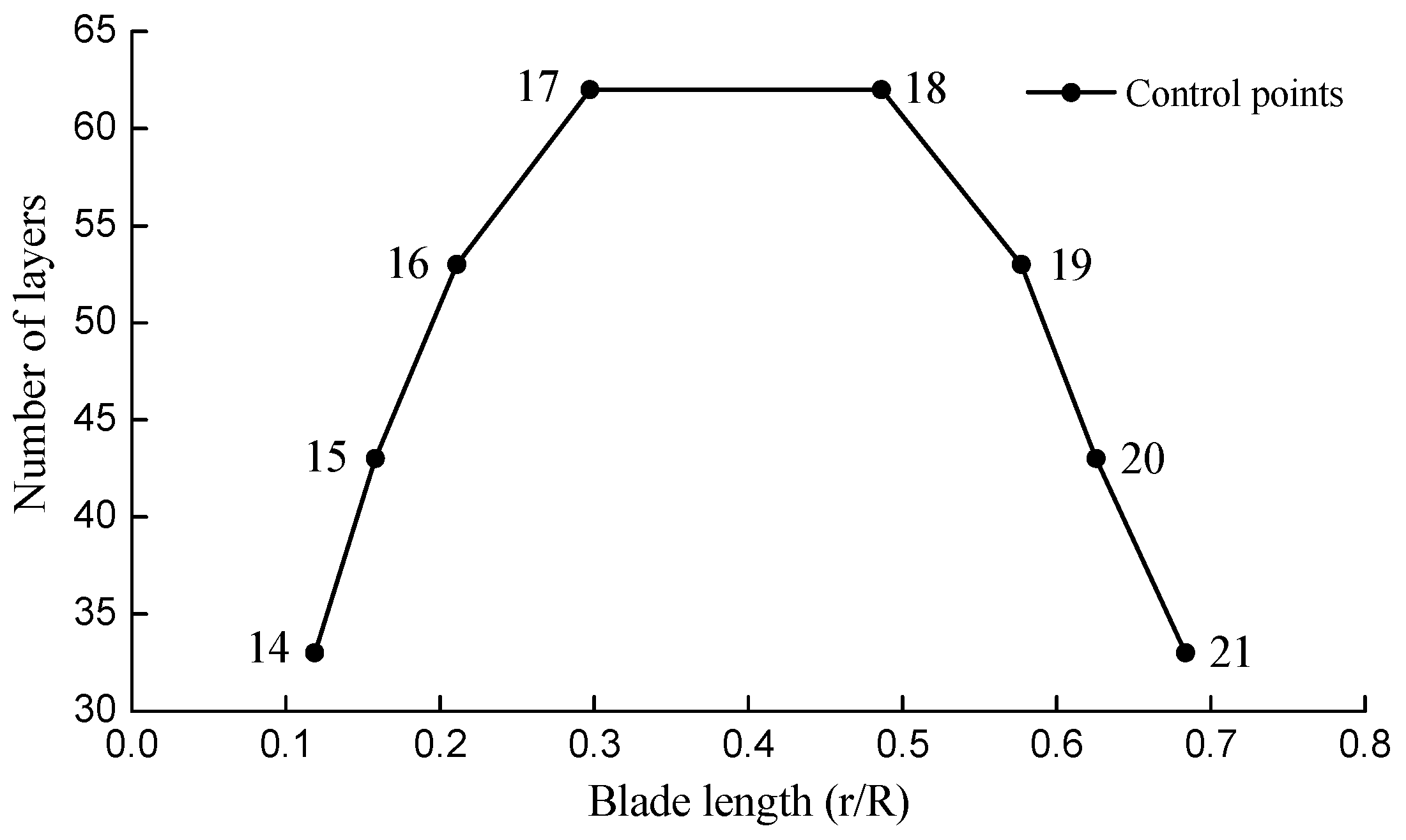
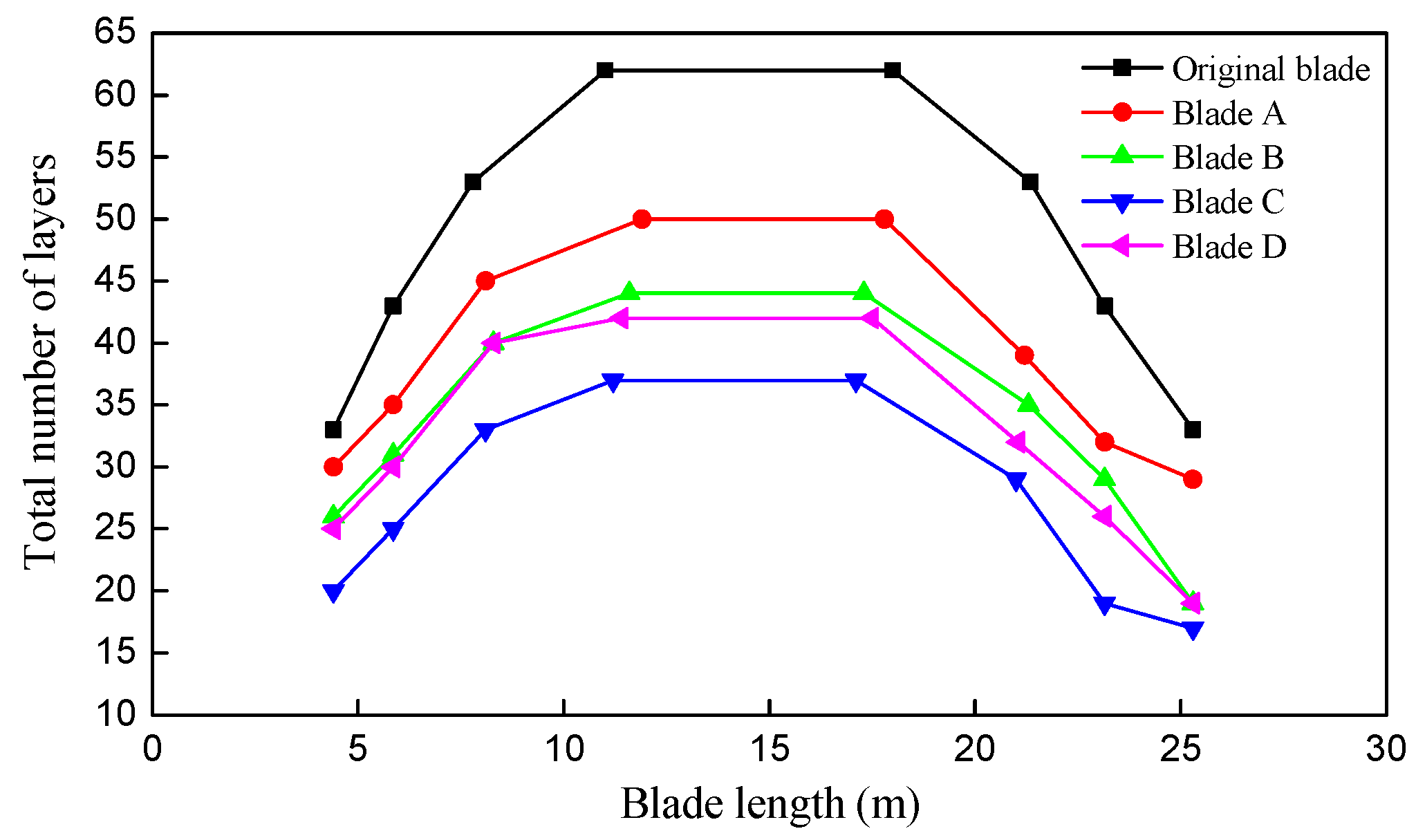
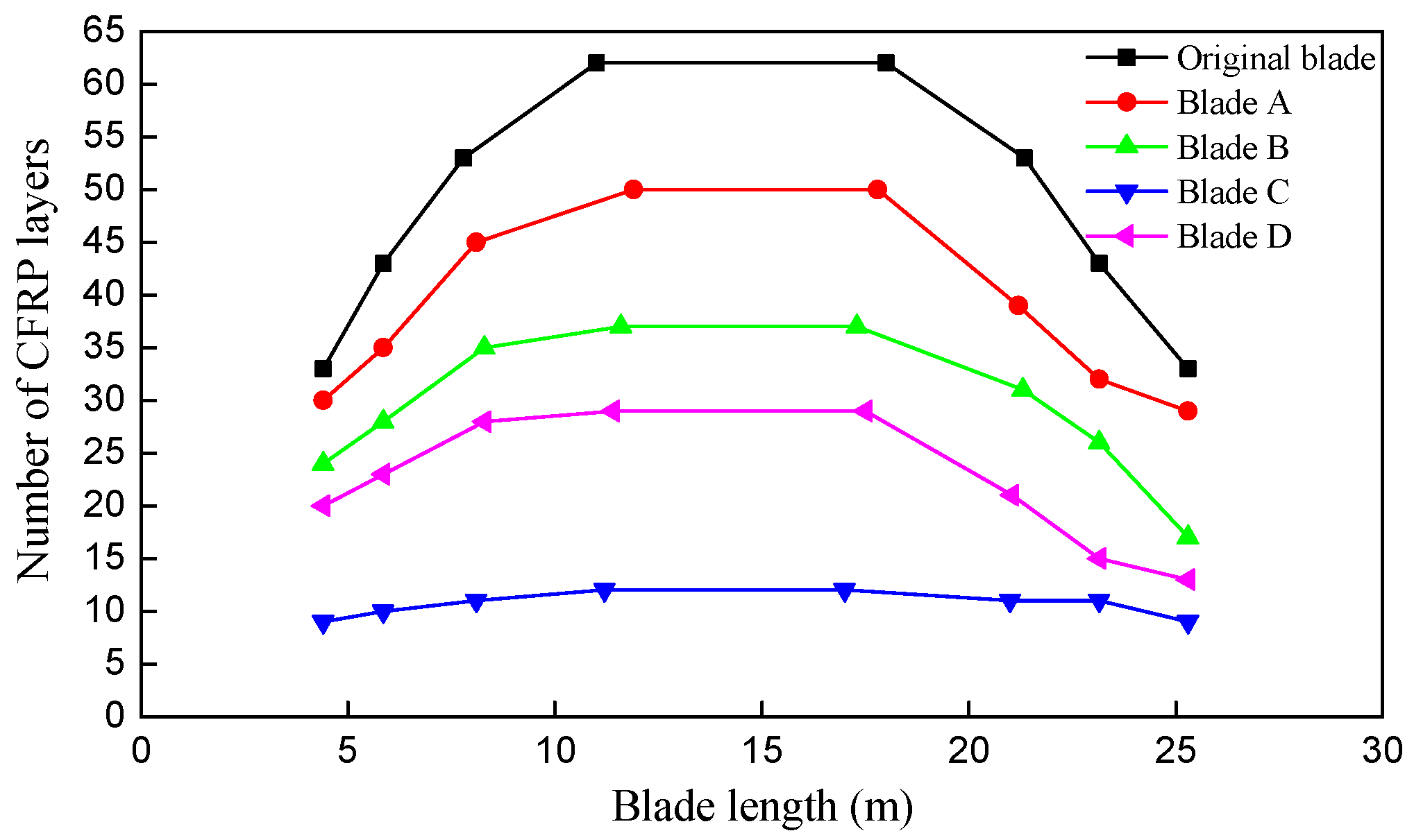
Figure 19 and Figure 20 show the comparisons of total material layup and GFRP layup in the spar cap between the original blade and optimized blades. It can be seen that the total number of layers and the number of GFRP layers both decrease obviously after optimization, especially in the middle part of the optimization region, while the number of CFRP layers gradually increases, and the region with maximum number of layers becomes smaller. It indicates that the materials in the middle part has greater impact on the blade mass and cost than those in the other parts. As the region close to the tip withstands smaller loads, the number of layers decrease a bit more than that close to the root.

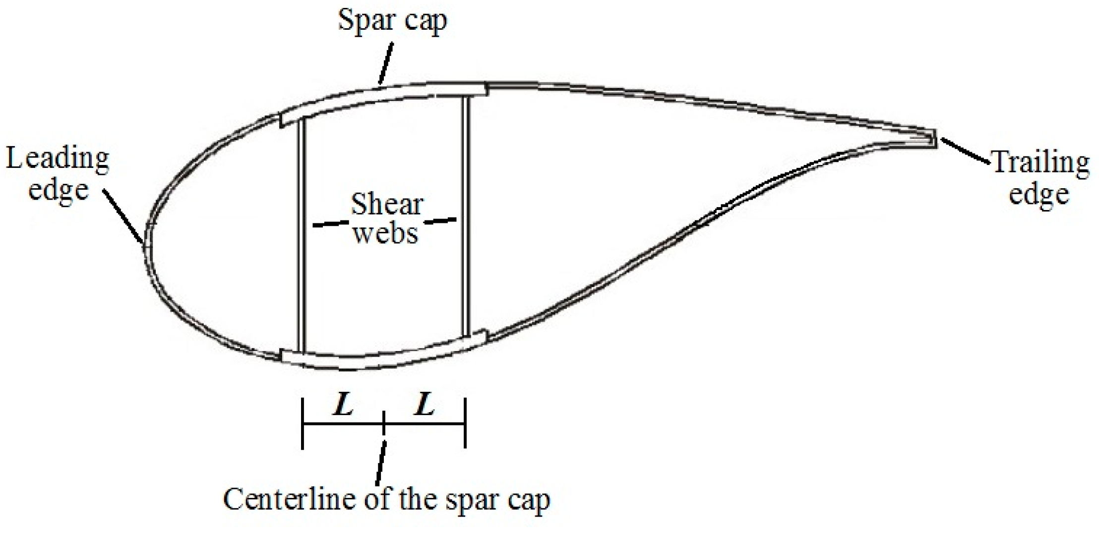
The position of the shear webs increases while the width of the spar cap decrease after optimization, as listed in Table 5. Moving away from the centerline of the spar cap can decrease the height of the shear webs, and a smaller width of the spar cap can reduce the amount of materials, which are both beneficial for reducing the blade mass and cost.

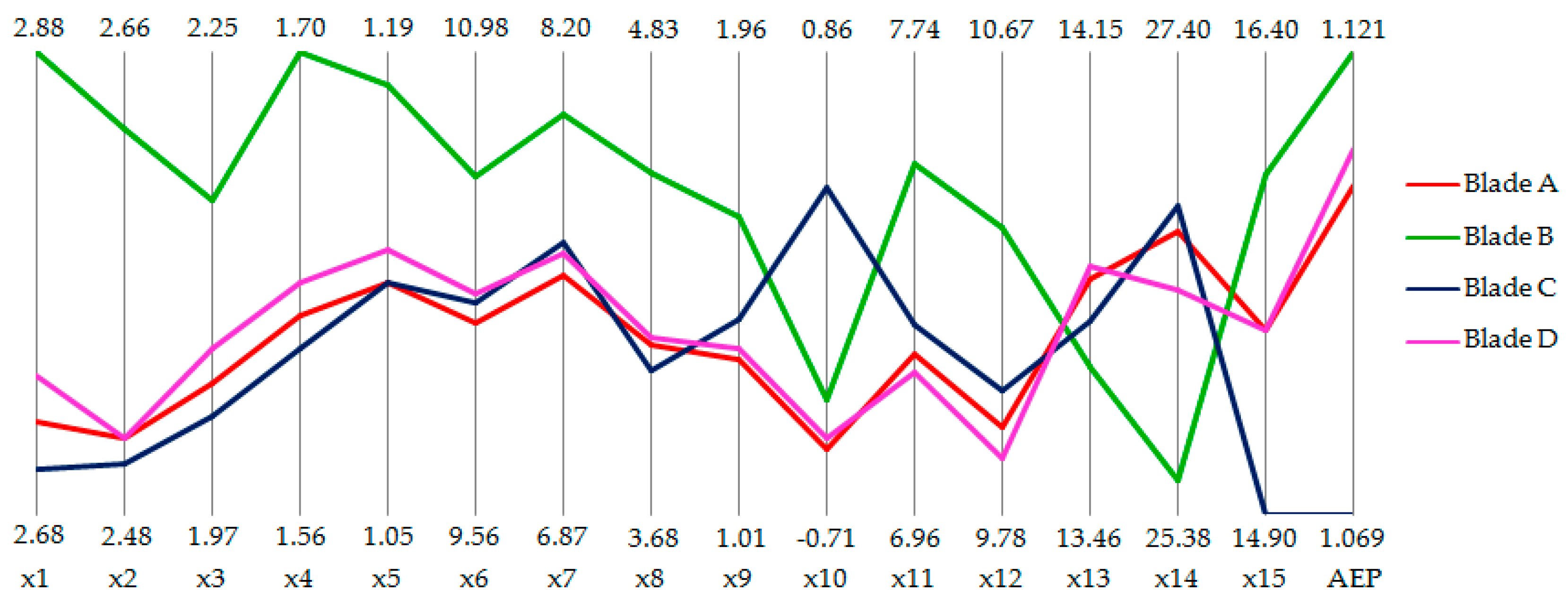
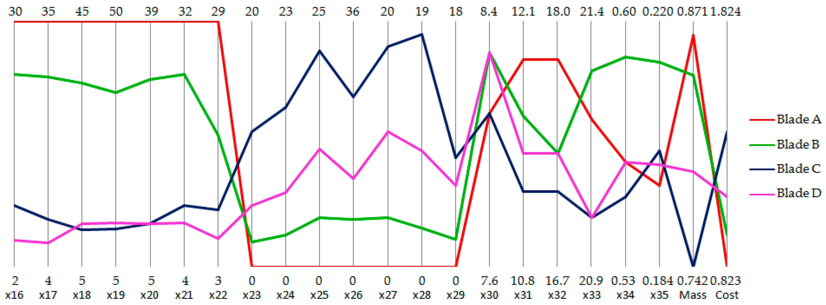
The parallel coordinates in the design space is applied again to find the blade designs with the improvements for the minimum mass objective and the minimum cost objective, as shown in Figure 21. The comparison shows that there are obvious differences for most structural variables between the three extreme point designs and the selected compromise design, the biggest differences are the number of material layers. Since CFRP is 10 times expensive than GFRP, more number of CFRP layers results higher cost, especially when the number of GFRP layers, chords and width of the spar cap are almost the same (blade C and D). The number of layers associated with the mass is on the contrary as CFRP is much lighter. On the other hand, because CFRP has higher modulus and tensile strength, its use can tremendously decrease the total number of layers and therefore reduce the cost to some extent, which means the cost of a blade design can be cheaper than the original blade when appropriate amount of GFRP combined with CFRP are applied.

The comparison in terms of the objective function can be found in Table 5. Compared with the original blade, the AEP of blades A, B, C and D increase by 10.6%, 12.1%, 6.9% and 11.0%, the blade mass decrease by 13.6%, 15.7%, 25.8% and 20.8%, and the blade cost reduce by 17.7%, 4.7%, −37.6% and −10.9%, respectively.

Table 6. Comparison of the structural behaviors under different load cases.

Blade	Optimization Region εmax		Non-Optimization Region εmax		dmax (m)		λ1		Fblade−1 (Hz)
	Case1	Case2	Case1	Case2	Case1	Case2	Case1	Case2
Original	0.00343	0.00429	0.00306	0.00407	3.71	4.60	2.024	2.466	1.027
A	0.00407	0.00494	0.00389	0.00480	3.52	4.43	1.206	1.617	1.229
B	0.00255	0.00339	0.00373	0.00473	2.73	3.80	1.510	1.845	1.567
C	0.00234	0.00318	0.00347	0.00412	1.66	2.51	1.883	2.190	1.987
D	0.00249	0.00330	0.00363	0.00448	2.38	3.32	1.688	1.983	1.744

lists the structural behaviors of the original and optimized blades under different load cases. It can be seen that the ultimate load case (case2) has a greater influence on most the structural behaviors, while the operational load case (case1) causes a smaller buckling eigenvalue, which is a result of the action of the normal and tangential forces. With the increase of CFRP layers, the maximum strains in the optimization and non-optimization regions and the tip deflection gradually decrease, the lowest buckling load factor and the first natural frequency increase. All of these are good for improving the blade strength, stiffness and reducing the response of the blade being excited. Since results such as blade B could improve not only the objectives but also the structural behaviors, they seem to be more desirable than the other results by the consideration of the purpose in the present work.

6. Conclusions and Future Work

This work presents a multi-objective aerodynamic and structural optimization method to design HAWT blades. A procedure mainly with an aerodynamic analysis model, a structural analysis model and a multi-objective optimization module is developed for this purpose. Three conflicting objectives: maximizing the AEP, minimizing the blade mass and cost are defined, the main aerodynamic and structural characteristics of the blade are selected as design variables and various design requirements are considered in the procedure.

A commercial 1.5 MW blade is applied as the baseline configuration, and the best trade-off solutions are obtained. For the airfoil-specific turbine blade, the results indicate that the maximum AEP requires larger chords, twists and the length of the main part that captures wind energy (approximately from the location of the 25% airfoil to the blade tip) and rotational speed; the minimization of blade mass requires smaller chords and width of the spar cap, less number of layers and more CFRP, while the minimizing blade cost asks for smaller chords and width of the spar cap, less number of layers and no CFRP. For the specific wind condition with a lower annual average wind speed, the aerodynamic performances of the optimized blades are significantly improved at low wind speeds. With the increase of CFRP layers, the structural behaviors can be improved. Satisfactory results to increase the AEP, and reduce the blade mass as well as cost are achieved, which shows the efficiency and reliability of the proposed procedure.

In order to further decrease the COE of blades, a more appropriate cost function including other factors such as production tooling, manufacturing labor and overland transportation need to be considered. Other competitive materials such as S-glass, carbon/wood hybrids and bamboo could also be considered. On the one hand, airfoils with higher lift-to-drag ratio can be used and the blade length can be changed to further improve the aerodynamic performances.