Article

Power Quality Disturbance Classification Using the S-Transform and Probabilistic Neural Network

1
School of Electrical Engineering and Automation, Tianjin University, Tianjin 300072, China
2
School of Control and Mechanical Engineering, Tianjin Chengjian University, Tianjin 300384, China
3
School of Electrical Engineering and Automation, Tianjin Polytechnic University, Tianjin 300387, China
*
Author to whom correspondence should be addressed.
Energies 2017, 10(1), 107; https://doi.org/10.3390/en10010107
Submission received: 19 September 2016 / Revised: 28 December 2016 / Accepted: 9 January 2017 / Published: 17 January 2017
(This article belongs to the Special Issue Distribution Power Systems and Power Quality)

Abstract

:
This paper presents a transient power quality (PQ) disturbance classification approach based on a generalized S-transform and probabilistic neural network (PNN). Specifically, the width factor used in the generalized S-transform is feature oriented. Depending on the specific feature to be extracted from the S-transform amplitude matrix, a favorable value is determined for the width factor, with which the S-transform is performed and the corresponding feature is extracted. Four features obtained this way are used as the inputs of a PNN trained for performing the classification of 8 disturbance signals and one normal sinusoidal signal. The key work of this research includes studying the influence of the width factor on the S-transform results, investigating the impacts of the width factor on the distribution behavior of features selected for disturbance classification, determining the favorable value for the width factor by evaluating the classification accuracy of PNN. Simulation results tell that the proposed approach significantly enhances the separation of the disturbance signals, improves the accuracy and generalization ability of the PNN, and exhibits the robustness of the PNN against noises. The proposed algorithm also shows good performance in comparison with other reported studies.

1. Introduction

In recent years, with the development and increasing implementation of distributed generation and micro-grids, large numbers of high-speed switching devices and non-linear converters are integrated into the power system. They are sources of power quality (PQ) disturbances such as sag, swell, interruption, flicker, harmonic, and oscillatory transients, etc. These voltage disturbances degrade the end user’s experience, and more importantly, it may damage modern precision devices and seriously affect the production efficiency of the manufacturing industry. Owing to the facts above, the problem of PQ disturbance detection and classification has received the attention of many scholars [1].
To understand the PQ disturbance, the time-frequency characteristics of disturbances signals need to be extracted and analyzed. Various signal processing algorithms, for example, Fourier transform (FT), short time Fourier transform (STFT) [2], wavelet transform (WT) [3,4], and Stockwell transform (S-transform) [5,6] have been utilized for this purpose. FT has the advantages of requiring a relatively less amount of calculation and broad applicability, however it has the disadvantages of spectrum leakage and fence effect, and it is limited to only detecting steady state signals. STFT transforms a signal into a two-dimensional complex function which reveals the frequency characteristics of the signal at each time instant, however its time window is relatively fixed and it is difficult to balance the frequency domain resolution and time domain resolution. WT can accurately detect the singular point and the time instant at which the PQ disturbance occurs, however it is time consuming and susceptible to noises. To overcome the disadvantages of the WT, Stockwell et al. [7] proposed the S-transform, which is conceptually a hybrid of STFT and WT. Compared with WT, S-transform can be treated as an extension of WT, on the other hand, S-transform can be treated as STFT with a variable window. S-transform has superior characteristics to WT and STFT, and it has good time-frequency focusing characteristics, satisfactory time-frequency resolution, and noise immunity. The features extracted with the S-transform of the disturbance signals are directly useable in intelligent algorithms for classification [8,9].
To make the S-transform more effective for different particular application focuses, various forms of S-transform have been proposed and examined. For example, to enable a flexible regulation of the time resolution and frequency resolution, a width factor is introduced into S-transform, which makes the width of Gaussian window adjustable. To have a better control over the scale and the shape of the analyzing window, a parameter P is introduced into the Gaussian window function [10,11,12]. Moreover, in [13], the frequency domain is segmented into domains of different frequencies, low, medium, and high. Within in different frequency domain, the width factor of the S-transform is different, which brings different time-frequency resolution the corresponding frequency domain, so the accuracy of PQ classification can be improved. In mechanical engineering, to analyze the vibration data, asymmetrical window function instead of the regular symmetrical one is used in S-transform [14]. To improve the ability for resolving signals whose frequency changes with time, a complex Gaussian window function is adopted in S-transform [15].
For PQ disturbance classification, it has been proven that S-transform-based approaches are effective, but efforts are needed to make them more favorable [16]. Conventionally, the S-transform used for this purpose takes its basic form—a symmetrical real Gaussian window function without a width factor or with a width factor but it takes a fixed value throughout. This paper studies how to make the S-transform more applicable to PQ disturbance classification by investigating its role in the S-transform-based classification approach. Specifically, an S-transform with a width factor is used; the determination of the value of the width factor is handled in a systemic view of the PQ disturbance classification problem itself. In other words, the width factor is treated as a variable. Its value is made to be feature oriented considering the fact that different features react to the time resolution or the frequency resolution differently.
As for the classification analysis, PNN is adopted in our study. The considerations are briefly given as follows. So far, various intelligent algorithms have been used to classify the PQ disturbances, for example, artificial neural network (ANN) [17], fuzzy logic [18], support vector machine (SVM) [19], etc. Artificial neural networks are mainly used for pattern matching, classification, function approximation, optimization, and data clustering. Neural networks have obvious advantages and have been widely used in PQ classification and fault diagnosis [20,21]. Multi-layer perceptron (MLP) and PNN are the typical forward neural network structures. Compared with MLP, PNN has many advantages such as simple structure, fast training rate, high accuracy, good generalization ability, and robustness, moreover, the training process of PNN is a single-pass network training stage without any iteration for weight adjustment, and it can be easily retrained to adapt to any network topology changes. In the comparison between PNN and the other two well-known neural networks i.e., feed forward multilayer (FFML) back propagation and learning vector quantization (LVQ), PNN provides better performance in terms of the classification results [16,19,22,23]. Based on the advantages of PNN and the characteristic of PQ disturbances, PNN is considered to be more favorable for PQ disturbances classification.
In summary, a PQ disturbance classification approach based on S-transform with a feature oriented regulatory and PNN is proposed and examined. Contents of sections below include: firstly, four features are selected through investigating the impacts of the width factor on the S-transform-Amplitude matrix of eight disturbance signals and the behavior of signal separation based on the features extracted; secondly, favorable value of the width factor used to extract each of the four features from the S-transform-amplitude matrix of disturbance signals is determined by examining the impacts of the width factor on the performance of PNN used for disturbance classification, and finally the proposed approach is tested, showing that it has higher classification accuracy and performs well with and without the noises.

2. Power Quality Disturbance Classification Based on Generalized S-Transform and Probabilistic Neural Network

In this section, first, the PQ disturbance classification algorithm based on S-transform and PNN is briefly described. Then, details of each functional unit of the algorithm are given, including the definition of eight disturbance signal types and the normal sinusoidal signal used in this study, mathematic description of S-transform without and with a width factor, definition of signal features and corresponding extraction formulation, and PNN. Finally, work of the authors is briefly introduced. Specifically, it is the implementation of the S-transform with a feature oriented optimal width factor to realize effective classification of the nine types of signals with a PNN.

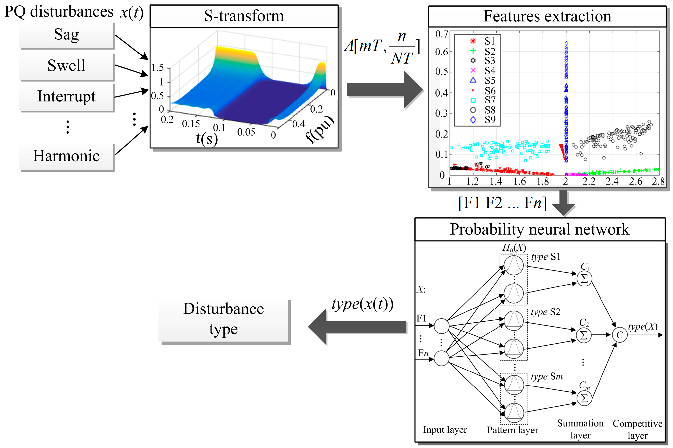
2.1. Method Overview

The PQ disturbance classification based on S-transform and PNN is illustrated in Figure 1. It contains three steps: (1) S-transform, by which the time and frequency information of the given PQ disturbance signal are obtained; (2) feature extraction, by which the customized feature vectors are further extracted from the time and frequency information obtained in step (1); (3) disturbance classification with PNN, the input of which is the feature vector of the PQ disturbance signal and the output of which is the disturbances classification result.

2.2. Disturbance Signal Types

IEEE Standard 1159 and the European standard EN50160 give definitions for various PQ disturbances and the corresponding suggested threshold settings [24,25]. For instance, Figure 2 shows the disturbance defined as a sag in the mentioned standards, which occurred to a normal sinusoidal voltage during the time approximately from 0.02 s to 0.14 s. The disturbance signal was captured on 21 March 2014 in Jurong East which located in the West Region of Singapore. The official source said it was due to a customer installation fault at Jurong Gateway Road. The PQ will be considered poor if the voltage magnitude is lower than the threshold set by the standard. In this specific case, the threshold should be 90% of the normal voltage magnitude.
Table 1 lists the PQ disturbance types considered in this paper. Each disturbance type is described with an equation with parameters, with which the disturbance generated comply with the corresponding disturbance defined in IEEE standard 1159-1995 [24]. S1, S2, …, and S8 denote sag, swell, interruption, flicker, oscillatory transient, harmonic, sag & harmonic, and swell & harmonic, respectively, S9 denotes normal signal. Where f = 50 Hz; ω = 2πf; T = 1/f. The parameters for the equations such as α, α3, α5, α7, t1, t2, αf, β, τ, fn are determined randomly within the thresholds.

2.3. Generalized S-Transform and Feature Extraction

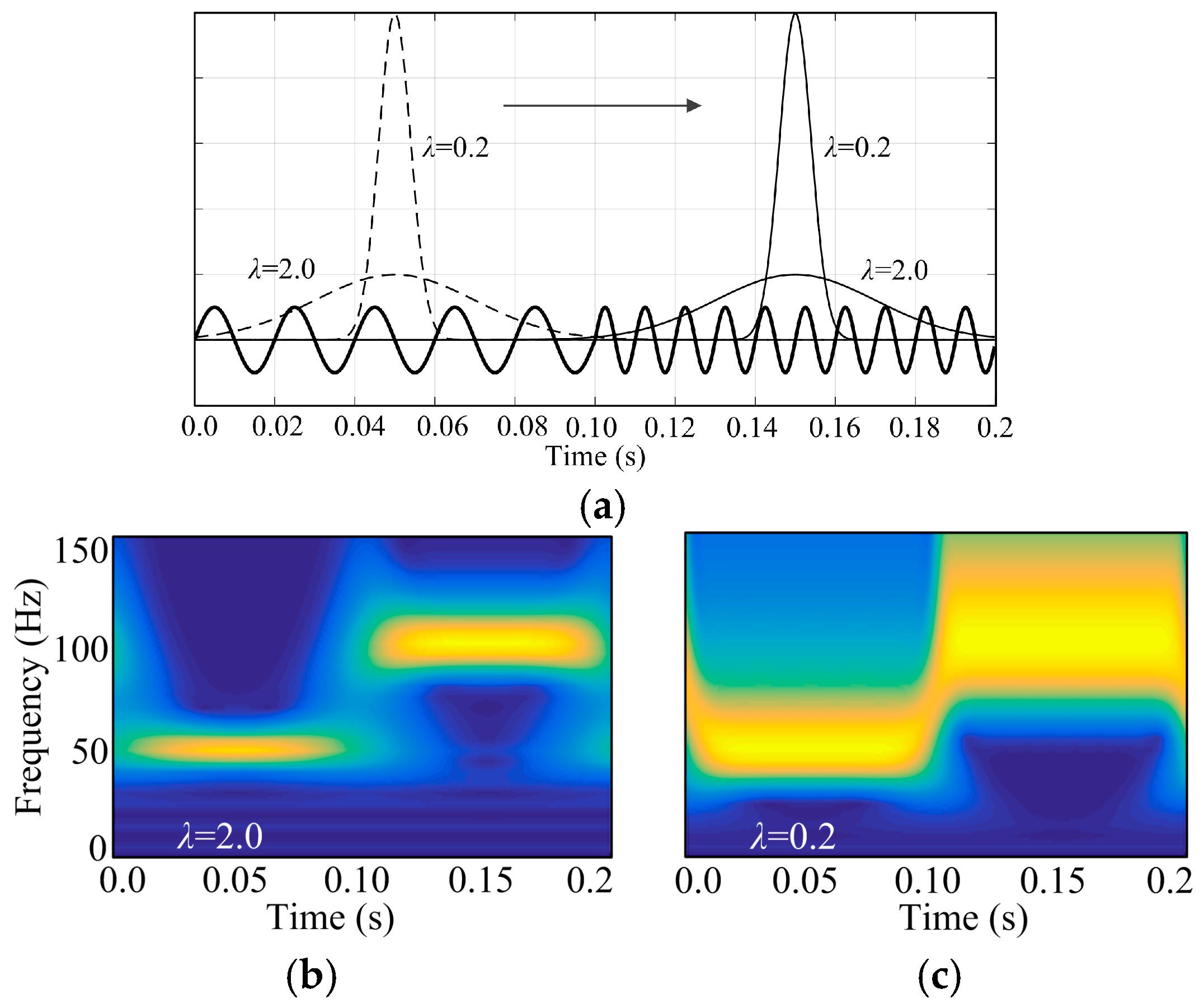
2.3.1. Generalized S-Transform

The continuous S-transform of signal x(t) is described as:
S ( τ , f ) = x ( t ) w ( τ t , f ) e i 2 π f t d t
where f is the frequency of signal x(t). w(τ − t, f) is Gaussian window function, it is defined as:
w ( τ t , f ) = 1 σ 2 π e ( τ t ) 2 2 σ 2
The S-transform matrix is a complex matrix whose rows pertain to frequency and columns to time. According to the Heisenberg principle, the time and frequency resolution cannot be improved at the same time. The intent of using the Gaussian window function in Equation (1) is to allow a better balancing between the time resolution and the frequency resolution. In Equation (2), τ is the point at the time axis at which the center of w(τ − t, f) sits. σ is a scale factor, it is defined as:
σ = 1 | f |
To make the Gaussian window function more effective, a width factor λ is introduced to Equation (3):
σ = λ | f |
Changing the value of λ adjusts the value of scale factor σ and therefore makes the width of Gaussian window function adjustable. If a value greater than 1 is assigned to λ, for the same frequency point, Gaussian window will be wider than in the case where λ takes a value of 1. Thus, higher frequency resolution can be achieved in time-frequency domain. Inversely, if a value less than 1 is assigned to λ, for the same frequency point, Gaussian window will be narrower than in the case where λ takes a value of 1. Thus, higher time resolution can be achieved in time-frequency domain.
For instance, Figure 3 shows the effect of width factor on the time-frequency analysis of S-transform. The source signal, as shown in Figure 3a consists of two sinusoidal signals of different frequencies, 50 Hz for the signal from time 0 to 0.1 s, 100 Hz for the signal from 0.1 to 0.2 s. Width factors under examination are 0.2 and 2.0. In the case of λ > 1.0, the Gaussian window will be wider and cover more line frequency cycles, and this will help to improve the accuracy of frequency analysis of the signal. However, a wider Gaussian window will not make it easy to identify the time instant at which the frequency of the signal changes. In the case of λ < 1.0, the Gaussian window will be narrower and cover fewer line frequency cycles, this will decrease the accuracy of frequency analysis of the signal, but a narrower Gaussian window will make it easy to identify the time instant at which the frequency of the signal changes.
The result presented in Figure 3b shows that by using a width factor greater than 1.0, the frequency of two sine signals can be satisfactorily identified, as seen the two thin frequency bands in sharp yellow, however, this brings more uncertainty on the time of the signal changes because the changing part of the two frequency bands is not clear. This indicates a width factor greater than 1.0 helps to achieve the better frequency resolution, but the time resolution will get worse. On the contrary, the result presented in Figure 3c shows that using a width factor less than 1.0, the frequency of two sine signals cannot be clearly identified, as seen the two thick frequency bands in sharp yellow, however, the changing part of the two frequency bands is clearly identified. This indicates a width factor less than 1.0 results unsatisfactory frequency resolution, but the time resolution will get better.
Substituting Equation (4) into Equation (1), the continuous generalized S-transform takes the form:
S ( τ , f ) = x ( t ) | f | λ 2 π e ( t τ ) 2 f 2 2 λ 2 e i 2 π f t d t
Then, with the definition τ = mT, f = n/NT, the discrete generalized S-transform expression can be obtained:
{ S [ m T , n N T ] = k = 0 N 1 X [ k + n N T ] e 2 π 2 λ 2 k 2 n 2 e i 2 π m k N n 0 S [ m T , 0 ] = 1 N k = 0 N 1 X [ k N T ] n = 0
where k, m, n = 0, 1, …, N − 1, N is the total number of sampling points. T is the time interval between two consecutive sampling points. X is the discrete Fourier transform.
Further, for the purpose of extracting the features of disturbance signals, the S-transform-Amplitude (STA) matrix is calculated as follows:
A [ m T , n N T ] = | S [ m T , n N T ] | m , n = 0 , 1 , , N 1

2.3.2. Feature Extraction

Feature extraction is one of the essential steps of PQ disturbance classification. Below are definitions of 10 features extracted from STA matrix.
F1: maximum amplitude of TmA-plot (time-maximum amplitude plot), and it has:
F 1 = max { T m A ( m ) }
where TmA-plot is maximum amplitude versus time by searching columns of STA matrix given in Equation (7) at every frequency, T m A ( m ) = max { A [ m T , n N T ] } .
F2: minimum amplitude of the TmA-plot:
F 2 = min { T m A ( m ) }
F3: mean value of the TmA-plot:
F 3 = 1 N m = 1 N T m A ( m )
F4: standard deviation of TmA-plot:
F 4 = 1 N m = 1 N ( T m A ( m ) F 3 ) 2
F5: the summation of the maximum and minimum of the TmA-plot:
F 5 = F 1 + F 2
F6: the standard deviation of FmA-plot (frequency maximum amplitude plot, which is maximum amplitude versus frequency by searching the rows of STA matrix at each time instant) for frequencies above four times the line frequency. It has:
F 6 = 1 N n = 1 N ( F m A ( n ) F m A ( n ) ¯ ) 2
where F m A ( n ) = max { A [ m T , n N T ] } with n N T > 200 , F m A ( n ) ¯ is the mean value of F m A ( n ) .
F7: the subtraction of the maximum and minimum of the FmA(n):
F 7 = max ( F m A ( n ) ) min ( F m A ( n ) )
F8: the Skewness of FmA-plot:
F 8 = 1 ( N 1 ) F 6 3 n = 1 N ( F m A ( n ) F m A ( n ) ¯ ) 3
F9: the Kurtosis of FmA-plot:
F 9 = 1 ( N 1 ) F 6 4 n = 1 N ( F m A ( n ) F m A ( n ) ¯ ) 4
F10: standard deviation of mr plot, where mr is time-amplitude plot determined by the frequency which has maximum amplitude in STA matrix above the frequency of 200 Hz, and it has
F 10 = 1 N m = 1 N ( m r ( m ) m r ( m ) ¯ ) 2
where m r ( m ) = A [ m T , n m r N T ] } , and n m r = arg max n { A [ m T , n N T ] } with n N T > 200 .
Apparently, when more features are used, a better classification effect may be expected. However, increasing the number of features results in a substantial increase of the calculation time as the scale of ANN used for disturbances classification will be increased. Therefore, the number of features used for the PQ disturbance classification should be as few as possible without obviously decreasing the classification accuracy. In this paper, four features are chosen according to the characteristic of disturbance and width factor, which are presented in Section 3.1.

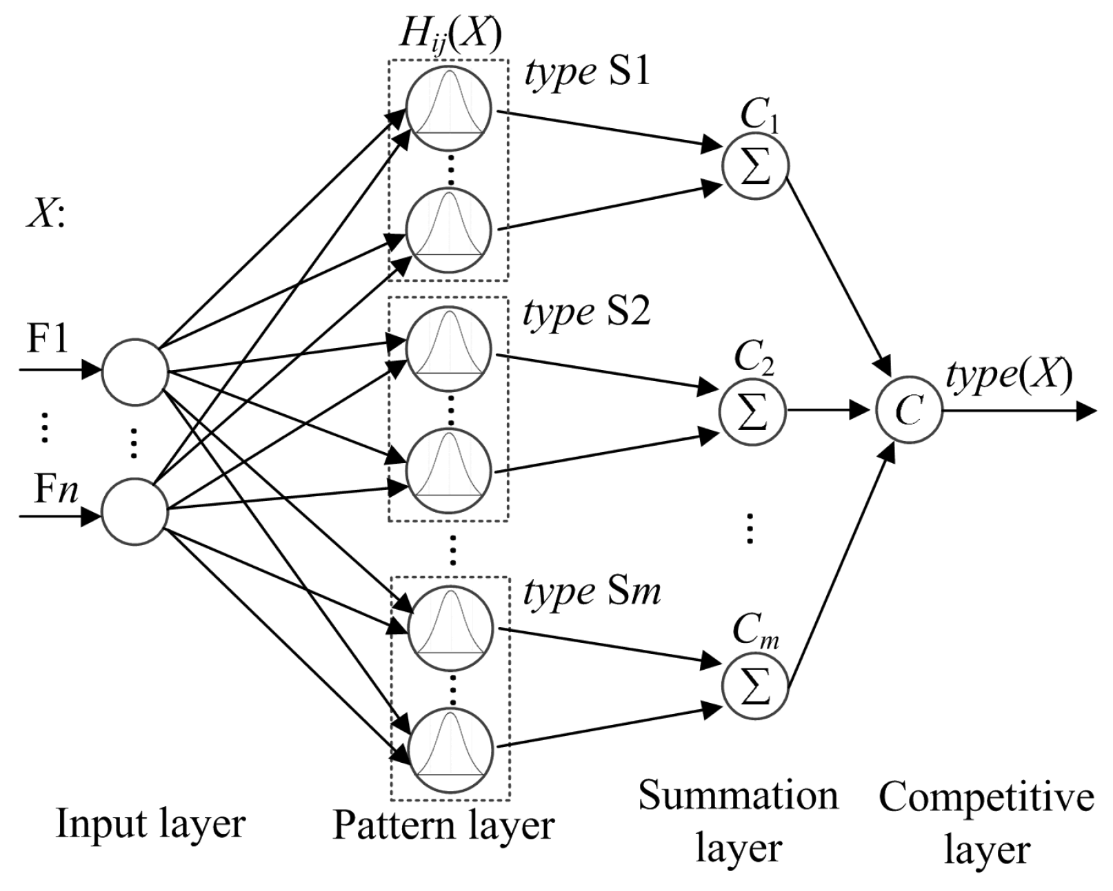
2.4. Probabilistic Neural Network

As shown in Figure 1, a vector of features selected is used to be the input of PNN. The output of PNN will be the disturbance type. Figure 4 shows the schematic diagram of PNN. It contains four layers: input layer, pattern layer, summation layer, and competitive layer. The function of each layer is as follows.
Pattern layer calculates Euclidean distance between the feature vectors of PQ disturbance testing sample X and every PQ disturbance training sample Xij, respectively. Below is the equation:
H i j ( X ) = 1 ( 2 π ) n / 2 δ n e X X i j 2 2 δ 2
where X = [F1 F2 F3 … Fn]T is the feature vector of an PQ disturbance testing sample, and F1, F2, F3, …, Fn are the features as defined in Section 2.3; n is the dimension of the feature vector; Xij is the feature vector of ith training sample of PQ disturbance type Sj, Sj∈ {S1, S2, …, S9}; δ is a smoothing parameter.
Summation layer makes summation of the results output from pattern layer, and the calculated conditional probability of X belonging to PQ disturbance type Sj is given below:
C j ( X ) = 1 N j i = 1 N j H i j ( X )
where Nj is the number of training samples belonging to PQ disturbance type Sj.
In the competitive layer, X is assigned to the PQ disturbance type with maximum conditional probability. It has:
t y p e ( X ) = arg max j { C j ( X ) }

3. Power Quality Disturbance Classification Based on Generalized S-transform with Feature Oriented Width Factor and Probabilistic Neural Network

The goal of this study is to realize an effective and efficient classification with high accuracy for eight types of disturbance signals plus the normal signal given in Section 2.2 using an approach based on the S-transform with a favorable width factor and PNN. Contents presented below include: selection of features used as inputs of PNN—four of ten are selected after examination; favorable value determination of the width factor for each of the four selected features by investigating the impacts of width factor on the PNN performance, and implementation of PNN for disturbance classification.

3.1. Method Proposed—Considering the Width Factor to Be Feature Oriented

In conventional PQ disturbance classification based on S-transform, the width factor λ is treated as a constant. In other words, all features interested are extracted from the S-transform matrix obtained with a width factor of the same value. Our studies, presented here, reveal that considering the width factor λ to be feature oriented renders a more satisfactory result. Implementation data and results presented below include: how does the STA-matrix of S-transform vary with λ, how does the effect of the feature separation behavior change with λ, and how does the classification accuracy of PNN vary with λ.

3.1.1. Effect of Width Factor on S-Transform-Amplitude-Matrix

Figure 5a–h shows the 3D plots of the STA-matrix of eight disturbance signals, listed in Table 1. For each disturbance signal, there are three 3D plots, which are graphical presentation of the STA-matrix obtained with three different values of the width factor λ, respectively. The STA-matrix is obtained per Equations (6) and (7); three values of λ are 0.1, 1.0, and 3.0. The values of λ, 0.1, 1.0, and 3.0 are selected per what was presented in Section 2.3.1: One less than 1.0, 0.1, which is used to examine its impacts on the low frequency domain resolution; one greater than 1.0, 3.0, which is used to examine its impacts on the high frequency domain resolution, and the value of 1.0, which is used as the base for comparison purpose.
3D plots in Figure 5 illustrate the behavior of the time-frequency characteristic of STA-matrix of each specific disturbance signal under the condition that different values of λ are used. This information helps to understand the advantages of introducing the width factor λ and the impacts of different λ values on distinguishing eight disturbance signals, S1 to S8.
Disturbance signals S1–S8 can be divided into three groups in terms of their characteristics: group 1 which has S1–S4, group 2 which has S5 and S6, and group 3 which has S7 and S8. The characteristic of group 1 is that the disturbances occur to the amplitude of the signals at the line frequency for a short period of time. Plots in Figure 5a, as an example, show the S-transform results of sag, and it can be seen that:
(1)
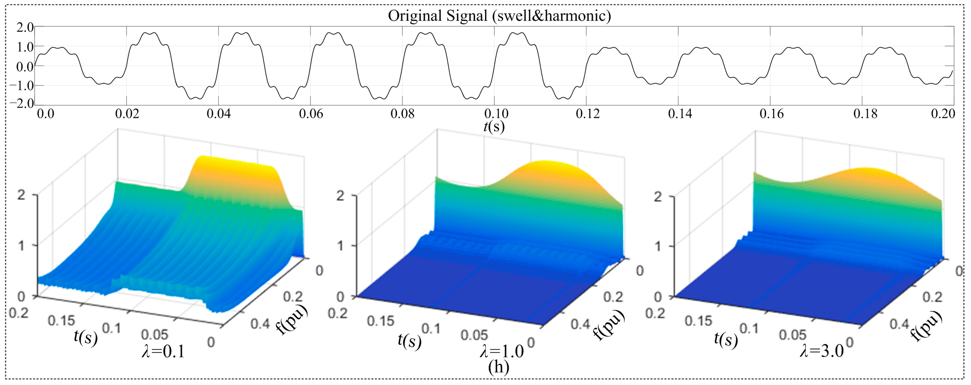
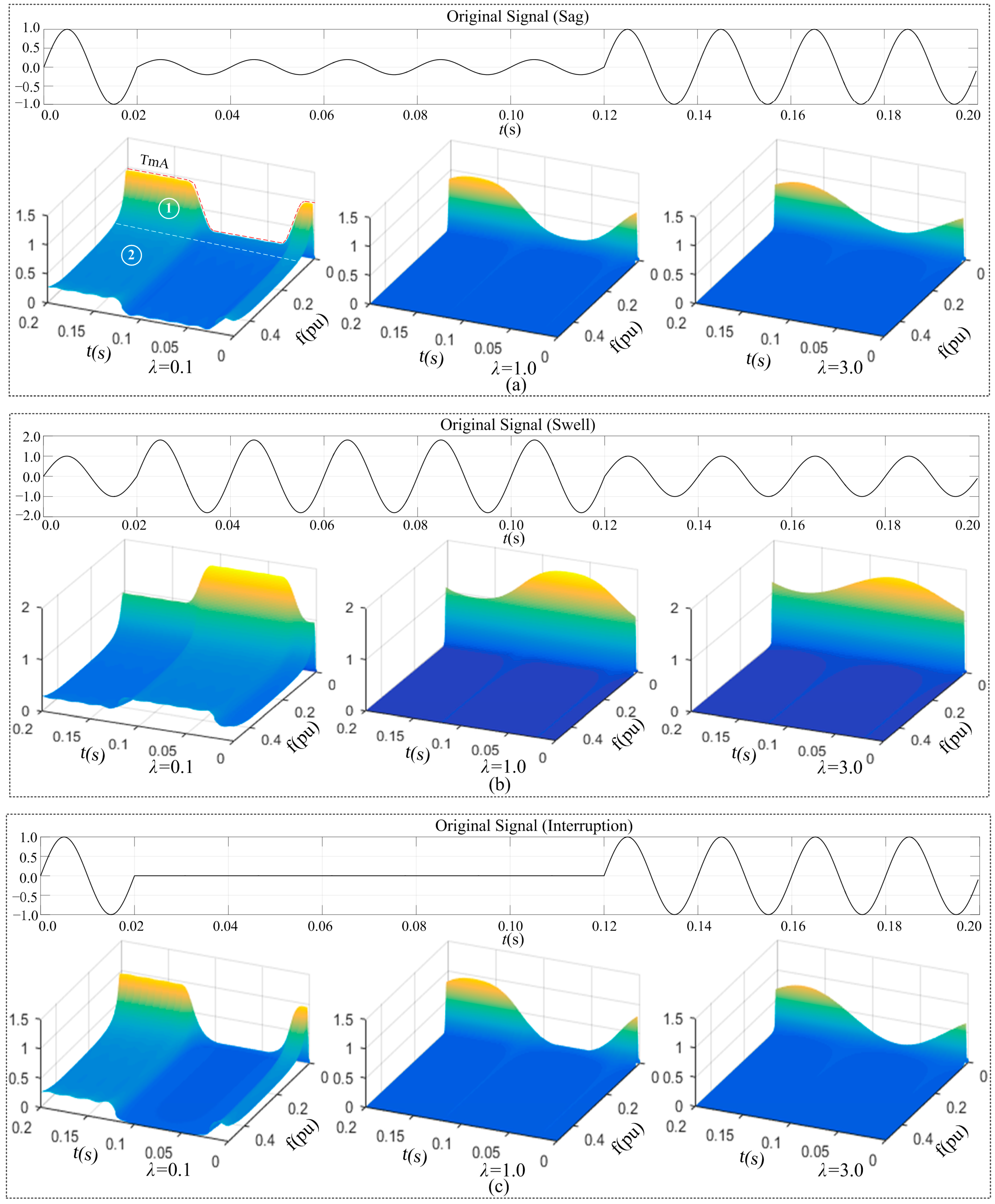
When the width factor takes a value less than 1.0, the contour (TmA curve) represent the actual behavior of sag at the line frequency (shown by ①). This indicates that higher time resolution of the STA matrix is achieved. In other words, a less than 1.0 value of λ results in a satisfactory presentation of the behavior of sag at the line frequency; however, in the high-frequency domain (shown by ②), a less than 1.0 value of λ decreases the frequency resolution of the STA matrix, as one can find that obvious fluctuation, which is not the characteristic of the sag, appears in the high-frequency domain. That is, a less than 1.0 value of λ results in a wrong presentation of the behavior of sag in the high-frequency domain.
(2)
When the width factor takes a value greater than 1.0, one can see that the high-frequency domain is almost flat without any high-frequency component, which is consistent with the actual behavior of sag in the high-frequency domain. This indicates that higher frequency resolution of the STA matrix is achieved. That is, a greater than 1.0 value of λ results a better presentation of the behavior of sag in the high-frequency domain. However, a greater than 1.0 value of λ decreases the time resolution of the STA matrix at the line frequency. It can be seen that the change of the TmA curve around line frequency becomes smoother, which may lead to a wrong identification of sag due to the inaccurate presentation of its amplitude variation with time. That is, a greater than 1.0 value of λ results an unsatisfactory presentation of the behavior of sag at line frequency. Similar conclusion can be obtained if examining plots in Figure 5b–d.
The characteristic of group 2 is that the disturbance appears to be the occurrence of harmonic components for a certain period of time or the harmonic components existing over the entire time range. The common feature of these two disturbance signal types is that the amplitude of the line frequency component of them stays unchanged. The difference between these two signals and the others are in the high-frequency domain. Plots in Figure 5e–f show the S-transform results of oscillatory transient and harmonic, and it can be seen that: (1) when the width factor takes a value less than 1.0, the frequency resolution of the STA matrix gets significantly reduced; High-frequency components which apparently do not belong to the original signals appear in the high-frequency domain; (2) these high frequency-components gradually fade away as λ increases. In the case when λ takes a value greater than 1.0, the high-frequency characteristics of the oscillatory transient and harmonic are well represented in the high-frequency domain.
Based on what are presented above, one can draw a conclusion that: A less than 1.0 value of λ results a better presentation of the behavior of the original signal at the line frequency, but distort the presentation of the behavior of the original signal in the high-frequency domain; A greater than 1.0 value of λ results a distorted presentation of the behavior of the original signal at the line frequency, but improves the presentation of the behavior of the original signal in the high-frequency domain. This indicates that combination of features is needed for the classification of different signals. As the signals of sag, swell, interruption, and flicker can be distinguished from others by the characteristic at the line frequency, a less than 1.0 value of λ is needed in the setting of the corresponding features; As the signals of oscillatory transient and harmonic can be distinguished from others by the characteristic in the high-frequency domain, a greater than 1.0 value of λ is needed in the setting of the corresponding features.
Characteristic of group 3 combines the characteristics of groups 1 and 2. Special attention needs to be paid to disturbance types S7 and S8, which are the combination of sag & harmonics and swell & harmonics, respectively. Investigation given above tells neither a value less than 1.0 nor a value greater than 1.0 ensures a successful separation of S7 or S8 form S1–S6, so in this condition, it needs combination of features to distinguish these disturbances from others.
In summary, to realize classification of the nine signal types defined in Table 1, a combination of features is needed; to make the classification more effective and efficient, making the width factor feature oriented may be considered.

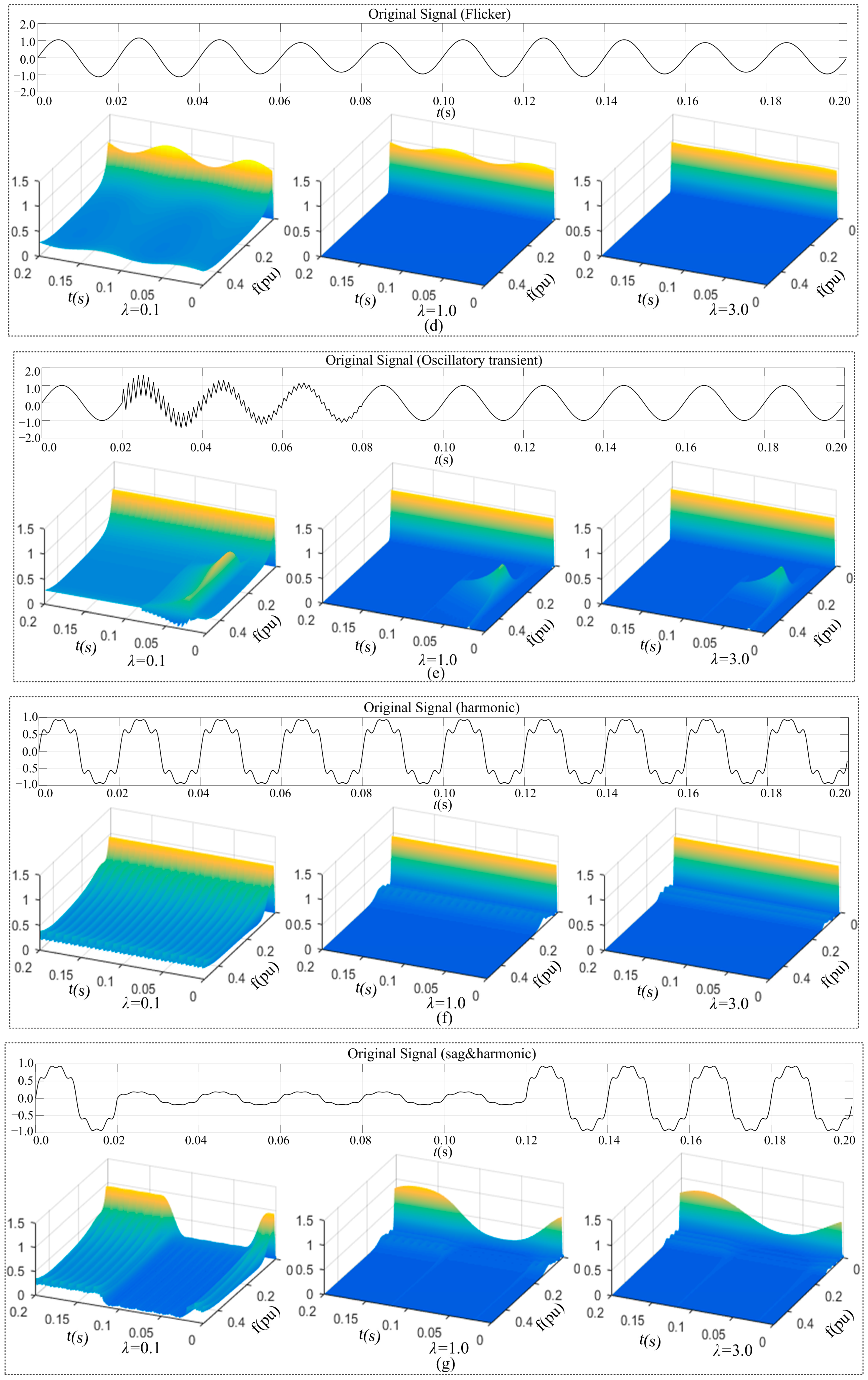
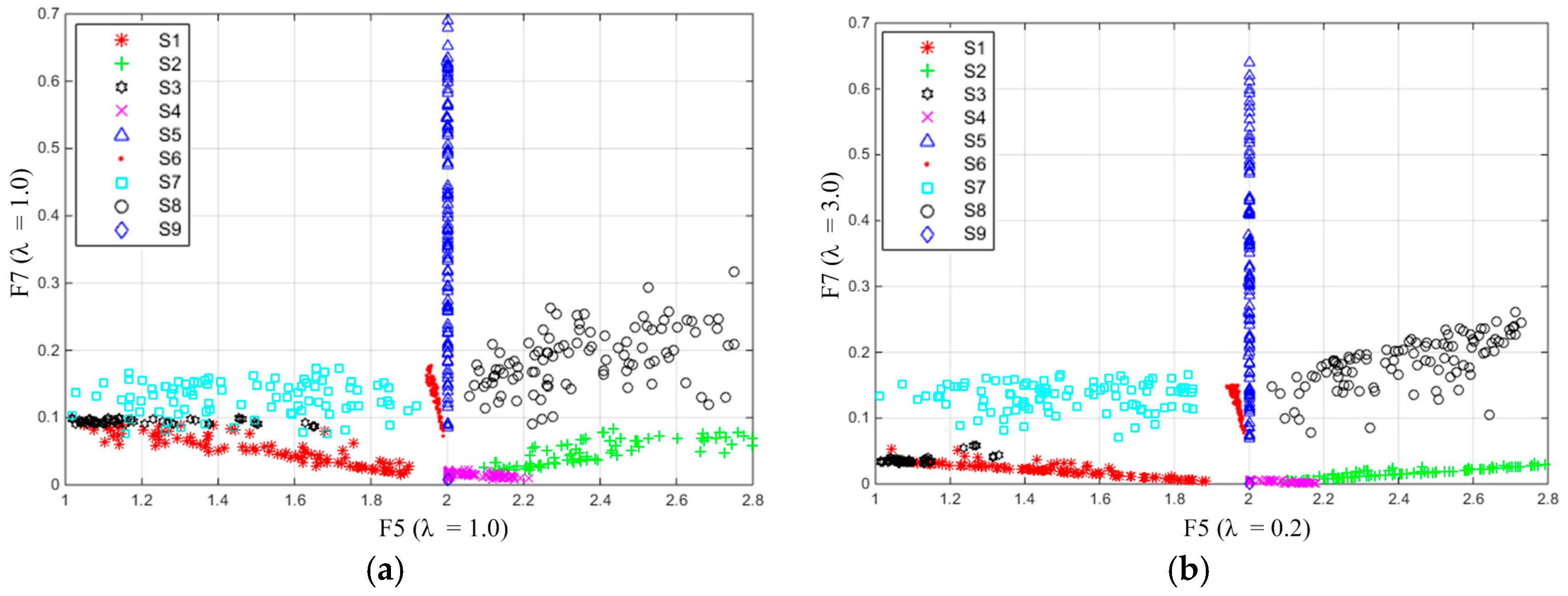
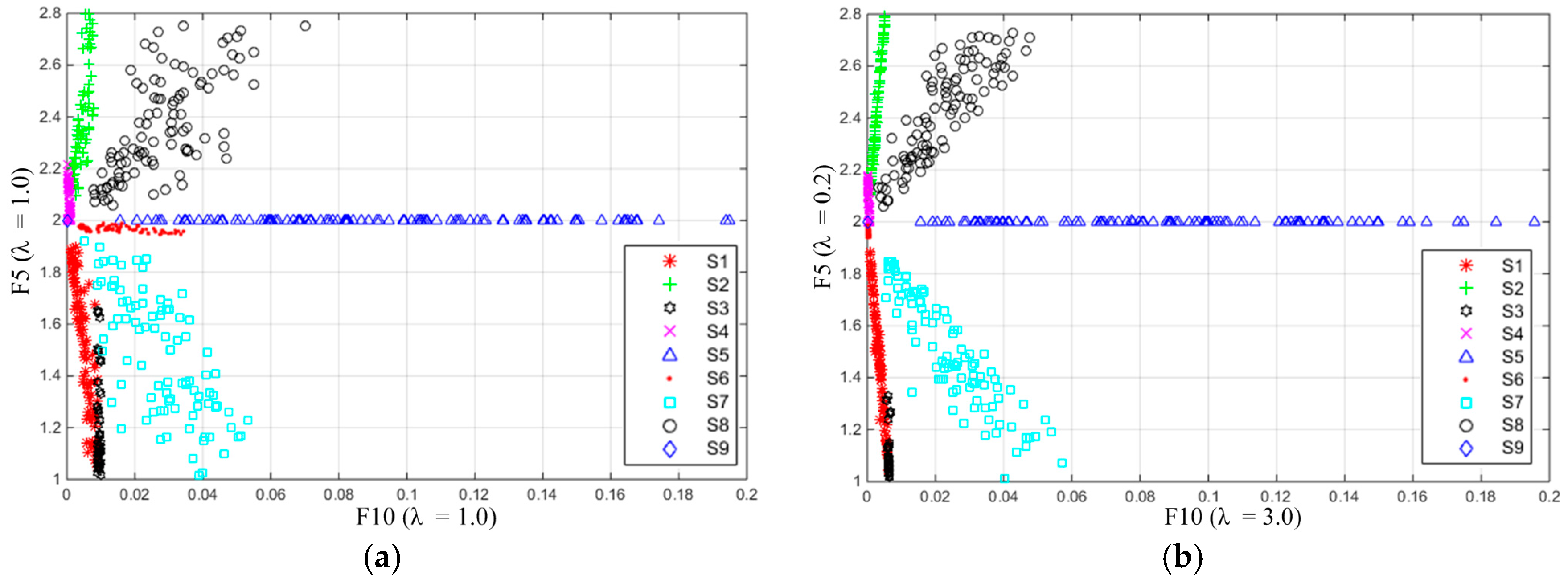
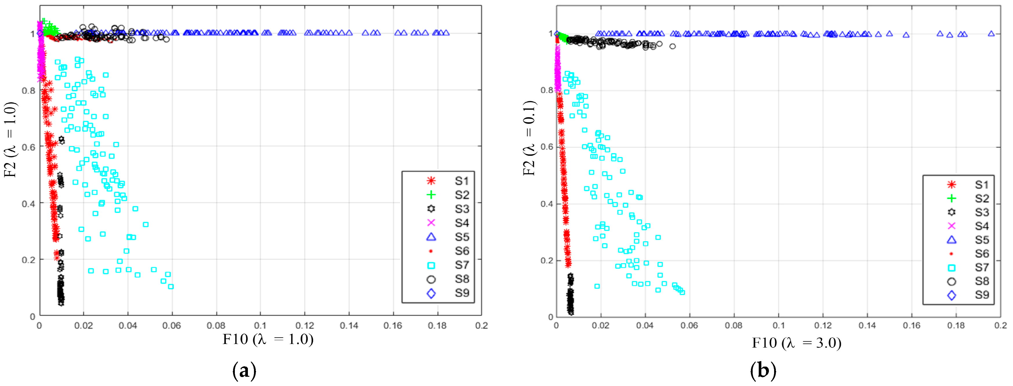
3.1.2. Effect of Width Factor on Feature Distribution Behavior

Different features represent different characteristics of signals. Among the 10 features defined in Section 2.3.2, features F1–F5, give an intuitive description of disturbance signals S1–S9 at the line frequency. Differently, features F6–F10, give an intuitive description of signals in the high-frequency domain. Specifically, F6–F9 expresses the frequency characteristic of signals in the high-frequency domain and F10 expresses the time characteristic of signals in the high-frequency domain. For a successful distinction of PQ disturbances S1–S9, commonly experienced in power system, a combination of features is needed per what are presented above. The goal is to use the least number of features to realize the classification with high accuracy. Various combination possibilities were examined. Combination of F2, F5, F7, and F10 was found to be the most applicable to our purpose:
(1)
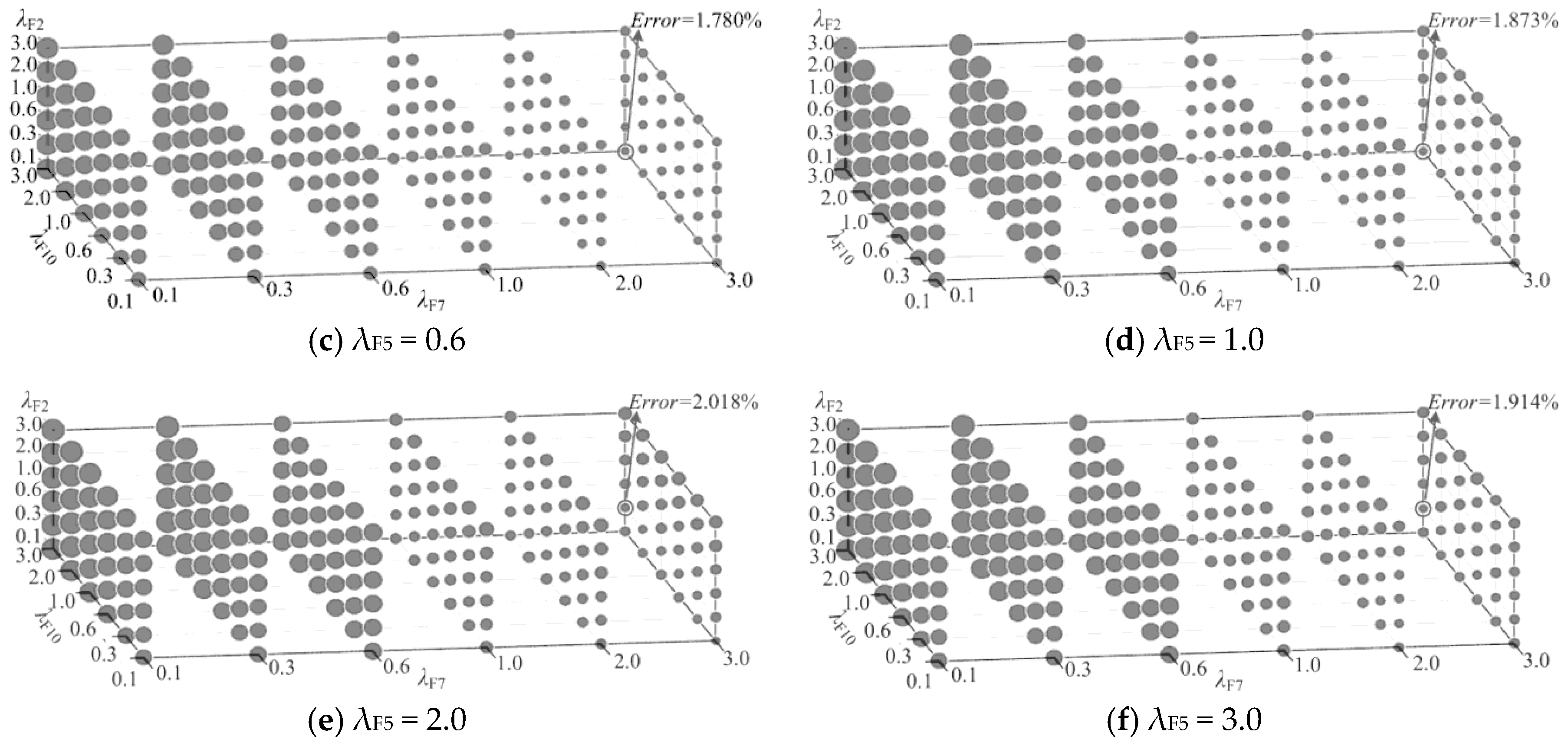
F2 and F5 embody the line frequency characteristics of disturbance signals. F2 contributes to the separation of normal signal, sag, swell, and interruption by assigning a value less than 1.0 to width factor λ. Additionally, F5 is used to distinguish flicker from others by assigning a value less than 1.0 to width factor λ.
(2)
F7 embodies the frequency characteristic characteristics of signals in the high-frequency domain, and it contributes to distinguishing S1–S4 (sag, swell, flicker and interruption) from S5–S6 (harmonic, transient oscillation) by assigning a greater than 1.0 value to width factor λ.
(3)
F10 embodies the time characteristic of signals in the high-frequency domain, and it contributes to the separation of transient oscillation and harmonic by assigning a greater than 1.0 value to width factor λ.
Based on the features F2, F5, F7, F10 above, firstly, to get intuitionistic vision, the distributions of PQ disturbances are shown in plots with the features combination F5 & F7, F5 & F10, F2 & F10. By analyzing the separation degree of eight types of PQ disturbances and the normal signal with different setting of λ (λF2, λF5, λF7, λF10), the distributions of PQ disturbances are shown in Figure 6, Figure 7 and Figure 8.
Figure 6 shows distributions of F5 & F7 of signals S1–S9. Figure 6a is the distribution obtained with both λF5 and λF7 taking a value of 1.0, which is the case of the features extracted from traditional S-transform. It shows that there is obvious overlapping between areas taken by S1, S3, and S7, respectively. Also, the areas taken by S2 and S8 respectively are too close to be easily separated. This will reduce the accuracy of classification algorithm. For comparison, Figure 6b shows the results obtained with λF5 = 0.2 and λF7 = 3.0, determined per discussion above. It can be seen that areas taken by S1, S3, and S7 are nicely separated, and there appears a clear space between areas taken by S2 and S8. Feature F7 is used to distinguish S1–S4 from S5–S6. Comparison between results obtained with λF7 = 1.0 and λF7 = 3.0, it can be seen the separation between S1–S4 and S5–S6 along the longitudinal axis (the direction of F7 axis) are much better in the case which λF7 is equal to 3.0.
Figure 7 shows distributions of F10 & F5 of signals S1–S9. Figure 7a is the distribution obtained with both λF10 and λF5 taking a value of 1.0. It shows that there are obvious overlapping between areas taken by S1, S3 and S7; Figure 7b shows the results obtained with λF10 = 3.0 and λF5 = 0.2. It shows that areas taken by S1, S2, S3, S7, S8 are nicely separated. F10 is used to separate transient oscillation S5 and harmonic S6, F2 and F10 distribution map given in Figure 7a shows that there is obvious overlapping between S5 and S6 along the horizontal axis (the direction of F10 axis) with λF10 = 1.0 while Figure 7b, there appears a clear space between areas taken by S5 and S6 with λF10 = 3.0.
Figure 8 shows distributions of F10 & F2 of signals S1–S9. Feature F2 contributes to the separation of normal signal, sag, swell and interruption. The result in Figure 8a shows that, along the longitudinal axis (the direction of F2 axis), there is obvious overlapping between areas taken by S1 and S3, and also some overlapping between areas taken by S2 and S4 with λF10 = 1.0; the result in Figure 8b shows that areas taken by S1 and S3, S2 and S4 are nicely separated with λF10 = 3.0. Moreover, comparison between Figure 8a,b says the S7 can be nicely separated from other signals with λF10 = 3.0, λF2 = 0.1.
In summary, results presented in Figure 6, Figure 7 and Figure 8 confirm that a combination of features is needed to separate S1 to S9. The results also verify that making λ feature oriented and using a favorable value instead of 1.0 for λ helps to achieve a satisfactory separation of S1–S9. In addition, for features which work better with λ greater than 1.0, λ values greater than 3.0 were tested and the result tells the improvement of the separation of signals S1 to S9 is insignificant. Similar results were obtained if values less than 0.1 are applied to λ for those features which work better with λ less than 1.0. Therefore, the variation range of λ used in the PNN section below is set to be from 0.1 to 3.0.

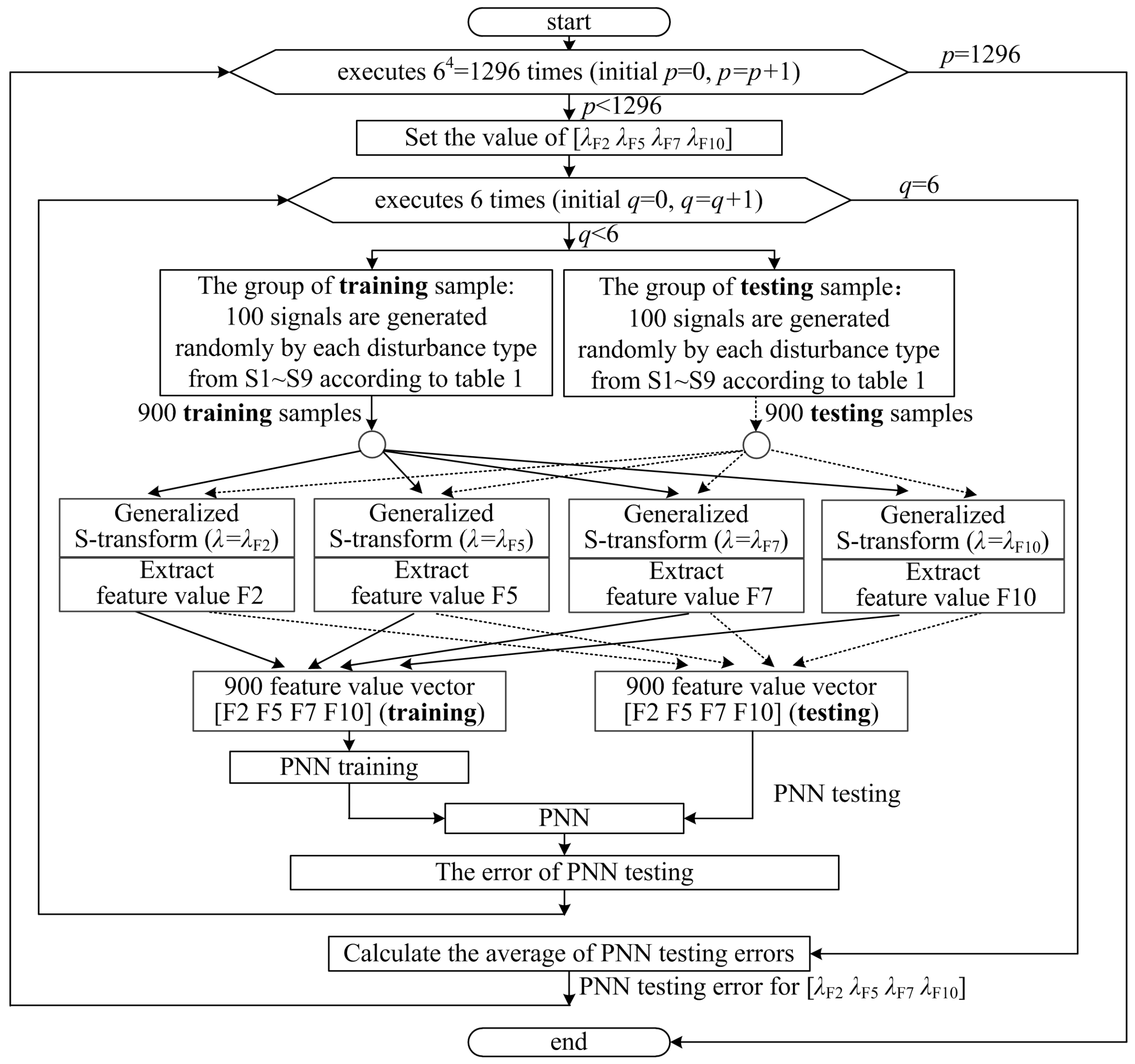
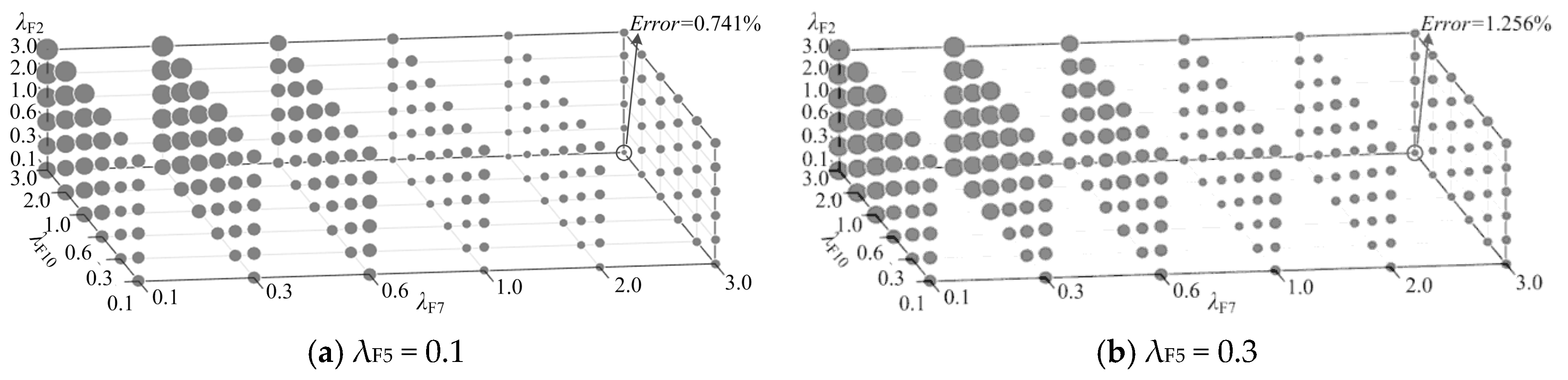
4. Determination of the Favorable Value of Feature Oriented Width Factor with the Use of Probabilistic Neural Network

This section presents the determination of favorable width factor set (λF2, λF5, λF7, and λF10) with PNN. Inputs of PNN are features F2, F5, F7, and F10 of the signal being classified. F2, F5, F7, and F10 are calculated from the S-transform matrix generated with width factor (λF2, λF5, λF7, and λF10); output of PNN is the classification result. The objective is to obtain the favorable value of (λF2, λF5, λF7, and λF10), with which and a trained PNN the classification of disturbances which falls into S1–S9 can be achieved with high accuracy. Steps for finding the favorable width factor (λF2, λF5, λF7, and λF10) are given in Figure 9.
64 = 1296 combinations of width factor λF2 λF5 λF7 λF10, see the external loop of the flowchart in Figure 9, are examined, which are generated by assigning each element of [λF2 λF5 λF7 λF10] with 0.1, 0.3, 0.6 1.0, 2.0, and 3.0, respectively. For each width factor combination set [λF2 λF5 λF7 λF10]: (1) in PNN training, 900 samples of signals are used, which are obtained by randomly generating 100 signals for each of nine signal types; in PNN testing, similarly, 900 randomly generated samples of signals are used; (2) the feature vectors [F2 F5 F7 F10] are extracted from the 1800 samples of signals by using the S-transform with the corresponding width factor combination [λF2 λF5 λF7 λF10]; (3) the PNN are trained and tested with the feature vectors [F2 F5 F7 F10] (900 for training; 900 for testing), and the classification error for the corresponding width factor combination [λF2 λF5 λF7 λF10] is evaluated.
In the process explained above, the 200 signals (100 for PNN training; 100 for PNN testing) of each disturbance type are generated by randomly selecting the value of parameters used by each disturbance signal type, seen the parameter column of Table 1. To mitigate the possible randomicity-related classification error, the internal loop is repeated six times, q = 6, as shown in the flowchart in Figure 9. The classification errors of PNN are calculated six times, and the average of the obtained six classification errors is taken as testing error of the PNN. The obtained testing errors of PNN are presented in Figure 10 with spheres, the size of which is proportional to the value of the corresponding error.
Firstly, take a look at Figure 10a. The size of spheres becomes smallest when λF2 takes the smallest value 0.1, λF7 and λF10 takes their greatest value 3.0. Similarity exists in Figure 10b–f. In other words, the smallest spheres on Figure 10a–f all locate at the lower right corner in the back. This tells us that favorable values for λF2, λF7 and λF10 are 0.1, 3.0, and 3.0, respectively. Then, comparing the size of the smallest sphere of each individual subfigure, one can see that the sphere at the lower right corner in the back of Figure 10a has the smallest size. This tells us that the PNN classification error becomes the least if λF5 takes a value of 0.1. Numbers in percentage format shown on the upper right corner in the back of each subfigure are the classification error of PNN corresponding to the sphere of the smallest size of each individual subfigure. It shows that the trained PNN will have the classification error be less than 1% (0.741% on Figure 10a) if λF2, λF5, λF7, and λF10 take their values to be 0.1, 0.1, 3.0, and 3.0, respectively. The trained PNN, with features F2, F5, F7, F10 as inputs, may provide a satisfactory classification of PQ disturbance S1 to S8 and the normal sinusoidal signal if F2, F5, F7, F10 are extracted from S-transform matrix obtained with width factors λF2, λF5, λF7, λF10 equal to 0.1, 0.1, 3.0, 3.0, respectively.

5. Accuracy of the Proposed Power Quality Disturbance Classification Approach

Without noise, classification results of PNN corresponding to the favorable width factor combination are shown in Table 2, and the classification accuracy is 99.259%. To analyze the effect of noise on the classification errors, different levels of noise are added to the nine types of signals. The results are listed in Table 3. The level of noise is expressed by the signal-to-noise ratio (SNR), and SNR = 20log10(AS/AN), where AS and AN are the maximum amplitude of the signal and noise, respectively.
As can be seen from Table 3, for the PQ disturbances without noise, the classification accuracy corresponding to the optimal width factor is 1.84%–7.86% higher than that of other width factor settings. The favorable width factor still maintains a good classification accuracy under noise (20 dB) and the classification accuracy is 2.21%–8.31% higher than the other width factor settings, including the traditional width factor settings ([λF2 λF5 λF7 λF10] = [1.0, 1.0, 1.0, 1.0]).

6. Performance Comparison

In order to evaluate the effectiveness and feasibility of the proposed algorithm, Table 4 shows the comparison between the obtained results in this paper and the reported results by other studies [4,8,16,17].
In [8,16], the classification accuracy of each PQ disturbance is lower than that of the proposed algorithm. For [4], the classification accuracy of each PQ disturbance is lower than that of the proposed algorithm except S7. For [17], the classification accuracy of each PQ disturbance is lower than that of the proposed algorithm, except for S1 and S2. The average classification accuracy shows the ratio of correctly classified PQ disturbances to the total number of PQ disturbances, and the proposed method gives the best classification results for this case.
The classification accuracy comparison between the proposed algorithm and other reported studies is shown in Table 5. For the PQ disturbances without noise, the classification accuracy corresponding to the proposed algorithm is 99.26% higher than that of other algorithms. For the PQ disturbances with low level noise condition (40 dB), the classification accuracy corresponding to the proposed algorithm is 99.13% slightly lower than that of the algorithm in [27], but higher than that of other algorithms. For the PQ disturbances with high level noise condition (30 dB), the classification accuracy corresponding to the proposed algorithm is 98.63% higher than that of other algorithms.

7. Conclusions

This paper proposed a PQ disturbance classification approach based on S-transform with a feature-oriented width factor and PNN. By introducing a width factor into the conventional S-transform, the time resolution and the frequency resolution presented by the STA matrix of the signal being analyzed is made adjustable. In this way, the impact of the width factor on the 3D-STA time-frequency magnitude spectrum of eight disturbance signals are studied and the overall picture of how the regulator factor affects the description accuracy of the signal in the low frequency domain and the high frequency domain is obtained. On the basis of this and according to the joint consideration of the characteristics of eight disturbance types in frequency domain and the definition of 10 features, four out of 10 features are selected to be used for the disturbance classification. Three combinations of four selected features are investigated in terms of the 2D distribution behavior of their values for the eight disturbance signal types; the influence of the width factor on the separation of data points denoting the values of each feature combination is presented. From there, association between each feature and the width factor value favorable for the corresponding feature is established. Further, it is verified with PNN by examining the classification accuracy with a wide variation range of each width factor, from 0.1 to 3.0. Furthermore, a PNN satisfactorily trained is obtained. Simulation tells it renders high classification accuracy (less than 1% error) for 8 type disturbance signals by using only four features as inputs, which are extracted from the S-transform amplitude matrix with corresponding favorable width factor. In addition, the obtained PNN shows satisfactory robustness under various noise conditions. Finally, the proposed algorithm shows better performance in comparison with those presented in other research studies.

Acknowledgments

The authors are grateful to the financial support from the Specialized Research Fund for National Key Research and Development Plan (No.2016YFB0900204), and doctoral Program of Higher Education of China (No. 20120032110070).

Author Contributions

The paper was collaborative effort among the authors. The authors contributed collectively to the theoretical analysis and manuscript preparations.

Conflicts of Interest

The authors declare no conflict of interest.

References

  1. Sainib, M.K.; Kapoora, R. Classification of quality disturbances event—A review. Int. J. Electr. Power Energy Syst. 2012, 43, 11–19. [Google Scholar] [CrossRef]
  2. Gu, Y.H.; Bollen, M.H.J. Time-frequency and time scale domain analysis of voltage disturbance. IEEE Trans. Power Deliv. 2000, 15, 1279–1284. [Google Scholar] [CrossRef]
  3. Biswal, B.; Biswal, M.; Hasanc, S. Nonstationary power signal time series data classification using LVQ classifier. Appl. Soft Comput. 2014, 18, 158–166. [Google Scholar] [CrossRef]
  4. Uyara, M.; Yildirim, S.; Gencoglu, M.T. An effective wavelet-based feature extraction method for classification of power quality disturbance signals. Electr. Power Syst. Res. 2008, 78, 1747–1755. [Google Scholar] [CrossRef]
  5. Uyara, M.; Yildirim, S.; Gencoglu, M.T. An expert system based on S-transform and neural network for automatic classification of power quality disturbances. Expert Syst. Appl. 2009, 36, 5962–5975. [Google Scholar] [CrossRef]
  6. Ray, P.K.; Kishor, N.; Mohanty, S.R. Islanding and power quality disturbance detection in grid-connected hybrid power system using wavelet and S-transform. IEEE Trans. Smart Grid 2012, 3, 1082–1094. [Google Scholar] [CrossRef]
  7. Stockwell, R.G.; Mansinha, L.; Lowe, R.P. Localization of the complex spectrum: The S-transform. IEEE Trans. Signal Process. 1996, 44, 998–1001. [Google Scholar] [CrossRef]
  8. Bhende, C.N.; Mishra, S.; Panigrahi, B.K. Detection and classification of power quality disturbances using S-transform and modular neural network. Electr. Power Syst. Res. 2008, 78, 122–128. [Google Scholar] [CrossRef]
  9. Dash, P.K.; Panigrahi, B.K.; Panda, G. Power quality analysis using S-transform. IEEE Trans. Power Deliv. 2003, 18, 406–411. [Google Scholar] [CrossRef]
  10. Pinnegar, C.R.; Mansinha, L. The S-transform with windows of arbitrary and varying shape. Geophysics 2003, 68, 381–385. [Google Scholar] [CrossRef]
  11. Djurović, I.; Sejdić, E.; Jiang, J. Frequency-based window width optimization for S-transform. Int. J. Electr. Commun. 2008, 62, 245–250. [Google Scholar] [CrossRef]
  12. Sejdić, E.; Djurović, I.; Jiang, J. A window width optimized S-transform. EURASIP J. Adv. Signal Process. 2007, 2008, 672941. [Google Scholar] [CrossRef]
  13. Huang, N.; Zhang, S.X.; Cai, G.W.; Xu, D.G. Power quality disturbances recognition based on a multiresolution generalized S-transform and a PSO-improved decision tree. Energies 2015, 8, 549–572. [Google Scholar] [CrossRef]
  14. McFadden, P.D.; Cook, J.G.; Forster, L.M. Decomposition of gear vibration signals by the generalized S-transform. Mech. Syst. Signal Process. 1999, 13, 691–707. [Google Scholar] [CrossRef]
  15. Pinnegar, C.R.; Mansinha, L. Time-local Fourier analysis with a scalable, phase-modulated analyzing function: The S-transform with a complex window. Signal Process. 2004, 84, 1167–1176. [Google Scholar] [CrossRef]
  16. Mishra, S.; Bhende, C.N.; Panigrahi, B.K. Detection and classification of power quality disturbances using S-transform and probabilistic neural network. IEEE Trans. Power Deliv. 2008, 23, 280–287. [Google Scholar] [CrossRef]
  17. Valtierra-Rodriguez, M.; Romero-Troncoso, R.D.J.; Osornio-Rios, R.A.; Garcia-Perez, A. Detection and classification of single and combined power quality disturbances using neural networks. IEEE Trans. Ind. Electr. 2014, 61, 2473–2481. [Google Scholar] [CrossRef]
  18. Biswal, B.; Dash, P.K.; Panigrahi, B.K. Power quality disturbance classification using fuzzy c-means algorithm and adaptive particle swarm optimization. IEEE Trans. Ind. Electr. 2009, 56, 212–220. [Google Scholar] [CrossRef]
  19. Mohanty, S.R.; Ray, P.K.; Kishor, N.; Panigrahic, B.K. Classification of disturbances in hybrid DG system using modular PNN and SVM. Electr. Power Energy Syst. 2013, 44, 764–777. [Google Scholar] [CrossRef]
  20. Kumar, R.; Singh, B.; Shahani, D.T.; Chandra, A.; Al-Haddad, K. Recognition of power-quality disturbances using S-transform -based ANN classifier and rule-based decision tree. IEEE Trans. Ind. Appl. 2015, 51, 1249–1258. [Google Scholar] [CrossRef]
  21. Meng, K.; Dong, Z.Y.; Wang, D.H.; Wong, K.P. A self-adaptive RBF neural network classifier for transformer fault analysis. IEEE Trans. Power Syst. 2010, 25, 1350–1360. [Google Scholar] [CrossRef]
  22. Specht, D.F. Probabilistic neural networks and the polynomial Adeline as complementary techniques for classification. IEEE Trans. Neural Netw. 1990, 1, 111–121. [Google Scholar] [CrossRef] [PubMed]
  23. Lin, W.M.; Lin, C.H.; Sun, Z.C. Adaptive multiple fault detection and alarm processing for loop system with probabilistic network. IEEE Trans. Power Deliv. 2004, 19, 64–69. [Google Scholar] [CrossRef]
  24. IEEE Recommended Practices for Monitoring Electric Power Quality; IEEE Std 1159-1995; IEEE-SASB Coordinating Committees: New York, NY, USA, 1995.
  25. EN 50160: Voltage Characteristics of Electricity Supplied by Public Distribution System; European Standards: Pilsen, Czech Republic, 2002.
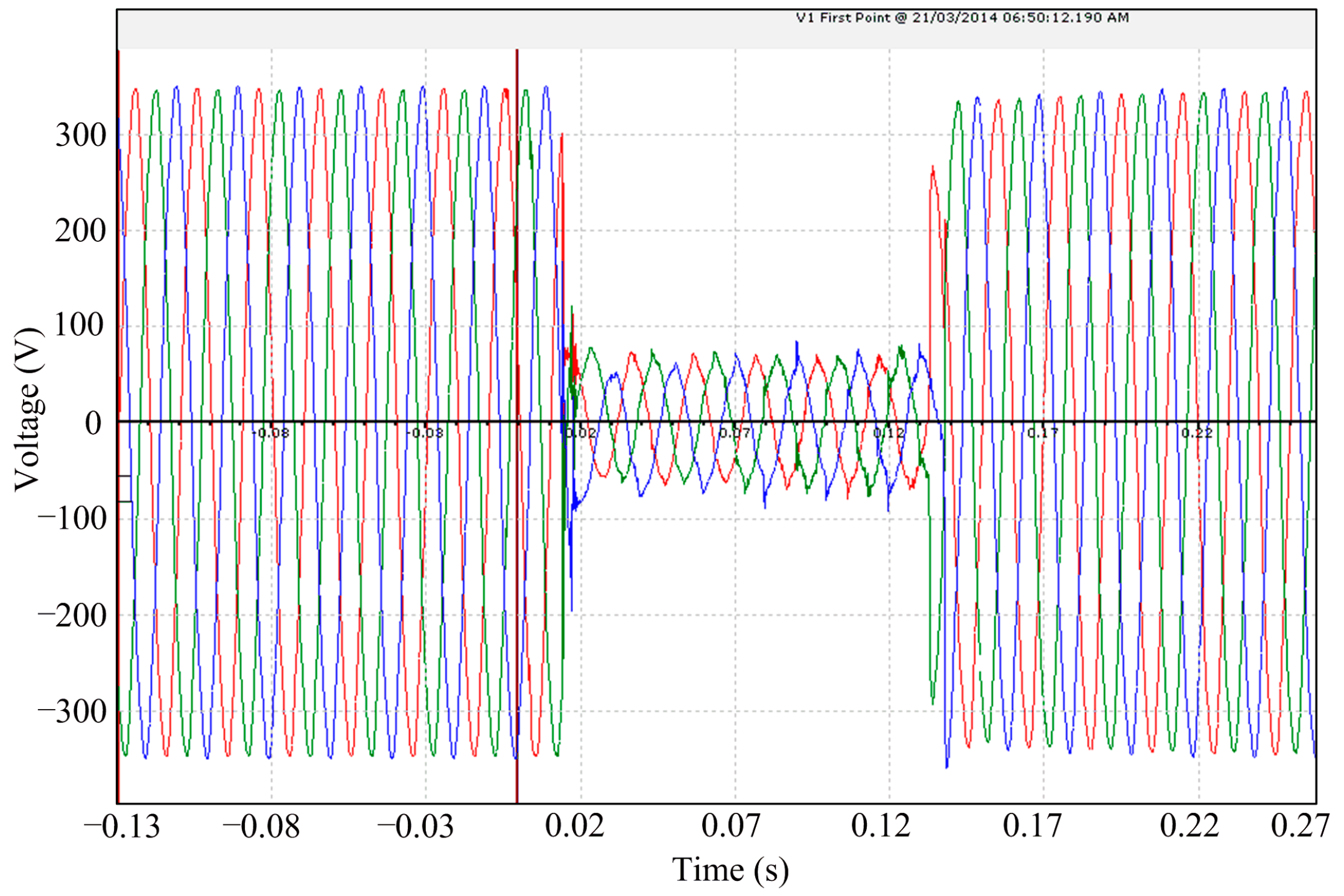
  26. Bohari, M.N. Voltage Dip 21/3/2014 0650hrs. Available online: http://powerquality.sg/wordpress/?p=194 (accessed on 21 March 2014).
  27. Zhao, F.Z.; Yang, R.G. Power-quality disturbance recognition using S-transform. IEEE Trans. Power Deliv. 2007, 22, 944–950. [Google Scholar] [CrossRef]
  28. Hooshmand, R.; Enshaee, A. Detection and classification of single and combined power quality disturbances using fuzzy systems oriented by particle swarm optimization algorithm. Electr. Power Syst. Res. 2010, 80, 1552–1561. [Google Scholar] [CrossRef]
  29. Biswal, M.; Dash, P.K. Detection and characterization of multiple power quality disturbances with a fast S-transform and decision tree based classifier. Digit. Signal Process. 2013, 23, 1071–1083. [Google Scholar] [CrossRef]
Figure 1. The schematic diagram of power quality (PQ) disturbance classification using S-transform and probabilistic neural network (PNN).
Energies 10 00107 g001
Figure 2. The waveform of sag captured from actual power system [26].
Energies 10 00107 g002
Figure 3. Time-frequency analysis results with different setting value of the width factor. (a) The comparison of the Gaussian windows with different width factor; (b) Time-frequency spectrum with λ = 2.0 and (c) Time-frequency spectrum with λ = 0.2.
Energies 10 00107 g003
Figure 4. The schematic diagram of PNN.
Energies 10 00107 g004
Figure 5. Disturbance signal and 3-D time-frequency magnitude spectrum. (a) sag; (b) swell; (c) interruption; (d) flicker; (e) oscillatory transient; (f) harmonic; (g) sag & harmonic; and (h) swell & harmonic.
Energies 10 00107 g005aEnergies 10 00107 g005bEnergies 10 00107 g005c
Figure 6. Comparison of F5 and F7 distribution behavior: (a) λF5 = 1.0, λF7 = 1.0; and (b) λF5 = 0.2, λF7 = 3.0.
Energies 10 00107 g006
Figure 7. Comparison of F5 and F10 distribution behavior: (a) λF10 = 1.0, λF5 = 1.0; and (b) λF10 = 3.0, λF5 = 0.2.
Energies 10 00107 g007
Figure 8. Comparison of F10 and F2 distribution behavior: (a) λF10 = 1.0, λF2 = 1.0; and (b) λF10 = 3.0, λF2 = 0.1.
Energies 10 00107 g008
Figure 9. The flow chart for the PNN classification error.
Energies 10 00107 g009
Figure 10. The error of PNN classification with the width factors combination [λF2 λF5 λF7 λF10] varying in the range of 0.1–3.0 (the smaller the radius of sphere, the smaller its corresponding classification error).
Energies 10 00107 g010aEnergies 10 00107 g010b
Table 1. Mathematical model of PQ disturbances.
SymbolType of Disturbance SignalEquationsParameters
S1Sag y ( t ) = ( 1 α ( u ( t t 1 ) u ( t t 2 )   )   ) sin ( ω t ) 0.1 α 0.9 , T t 2 t 1 9 T , t 1 t 2
S2Swell y ( t ) = (   1 + α (   u ( t t 1 ) u ( t t 2 )   )   ) sin ( ω t ) 0.1 α 0.8 , T t 2 t 1 9 T
u ( t ) = { 1 t 0 0 t < 0
S3Interruption y ( t ) = (   1 α (   u ( t t 1 ) u ( t t 2 )   )   ) sin ( ω t ) 0.9 α 1 , T t 2 t 1 9 T
S4Flicker y ( t ) = (   1 + α f sin ( β ω t )   ) sin ( ω t ) 0.1 α f 0.2 ,   5 Hz β 20 Hz
S5Oscillatory transient y ( t ) = sin ( ω t ) + α e ( t t 1 ) / τ sin ω n ( t t 1 ) ( u ( t 2 ) u ( t 1 ) ) 0.1 α 0.8 ,   0.5 T t 2 t 1 3 T , 8 ms τ 40 ms ,   300 Hz f n 900 Hz
S6Harmonic y ( t ) = α 1 sin ( ω t ) + α 3 sin ( 3 ω t ) + α 5 sin ( 5 ω t ) + α 7 sin ( 7 ω t ) 0.05 α 3 0.15 ,   0.05 α 5 0.15 , 0.05 α 7 0.15 ,   α i 2 = 1
S7Sag and harmonic y ( t ) = ( 1 α ( u ( t t 1 ) u ( t t 2 ) ) )   ( α 1 sin ( ω t ) + α 3 sin ( 3 ω t ) + α 5 sin ( 5 ω t ) ) 0.1 α 0.9 ,   T t 2 t 1 9 T , 0.05 α 3 0.15 , 0.05 α 5 0.15 , α i 2 = 1
S8Swell and harmonic y ( t ) = ( 1 + α ( u ( t t 1 ) u ( t t 2 ) ) ) ( α 1 sin ( ω t ) + α 3 sin ( 3 ω t ) + α 5 sin ( 5 ω t ) ) 0.1 α 0.8 ,   T t 2 t 1 9 T , 0.05 α 3 0.15 , 0.05 α 5 0.15 , α i 2 = 1
S9Normal sine y ( t ) = sin ( ω t ) -
Table 2. PNN classification results with the favorable width factor combination.
CategoryS1S2S3S4S5S6S7S8S9Accuracy
S15920800000098.67%
S205830170000097.17%
S300600000000100%
S40905910000098.50%
S500006000000100%
S600000600000100%
S76000005940099.00%
S800000006000100%
S900000000600100%
PNN classification accuracy = 99.259%
Table 3. PNN classification accuracy with noise conditions.
λF2, λF5, λF7, λF10PNN Classification Accuracy (%)
Pure40 dB30 dB20 dB
0.1, 0.1, 3.0, 3.099.2699.1398.6398.38
1.0, 1.0, 1.0, 1.096.9296.7896.6595.94
0.1, 2.0, 3.0, 0.697.4296.8096.6296.17
2.0, 1.0, 0.1, 1.091.4091.2791.0090.07
3.0, 1.0, 2.0, 1.097.0495.9895.8795.68
Table 4. Performance comparison in terms of percentage of correct classification results.
CategoryClassification Accuracy (%)
Proposed Method[4][8][16][17]
S198.67889895100
S297.1796.59291100
S310085.5510099100
S498.50-989894
S5100-10010098
S6100100929698
S799.00100939898
S8100100909897
S9100100100100100
Average classification accuracy99.2695.7195.597.2298.33
Table 5. Comparison between the proposed algorithm and other algorithms with noise conditions.
PQ Classification StudiesClassification Accuracy (%)
Pure40 dB30 dB
[4]95.7193.6491.85
[27]-99.798.5
[28]98.596.87593.625
[29]-98.897.49
Proposed method99.2699.1398.63

