Article

Exploring the Feasibility of Low-Carbon Scenarios Using Historical Energy Transitions Analysis

1
Grantham Institute, Imperial College London, South Kensington Campus, London SW7 2AZ, UK
2
Met Office Hadley Centre, FitzRoy Road, Exeter, Devon EX1 3PB, UK
3
Department of Chemical Engineering, Imperial College London, South Kensington Campus, London SW7 2AZ, UK
*
Author to whom correspondence should be addressed.
Energies 2017, 10(1), 116; https://doi.org/10.3390/en10010116
Submission received: 31 October 2016 / Revised: 13 December 2016 / Accepted: 5 January 2017 / Published: 18 January 2017
(This article belongs to the Special Issue Low Carbon Economy)

Abstract

:
The scenarios generated by energy systems models provide a picture of the range of possible pathways to a low-carbon future. However, in order to be truly useful, these scenarios should not only be possible but also plausible. In this paper, we have used lessons from historical energy transitions to create a set of diagnostic tests to assess the feasibility of an example 2 °C scenario (generated using the least cost optimization model, TIAM-Grantham). The key assessment criteria included the rate of deployment of low carbon technologies and the rate of transition between primary energy resources. The rates of deployment of key low-carbon technologies were found to exceed the maximum historically observed rate of deployment of 20% per annum. When constraints were added to limit the scenario to within historically observed rates of change, the model no longer solved for 2 °C. Under these constraints, the lowest median 2100 temperature change for which a solution was found was about 2.1 °C and at more than double the cumulative cost of the unconstrained scenario. The analysis in this paper highlights the considerable challenge of meeting 2 °C, requiring rates of energy supply technology deployment and rates of declines in fossil fuels which are unprecedented.

1. Introduction

Most of the mitigation scenarios developed by the scientific community, as presented and discussed, for example, in the Intergovernmental Panel on Climate Change (IPCC)’s fifth assessment report [1], use energy systems models (which, as part of integrated assessment models, are often combined with modules that calculate the climate impact of greenhouse gas emissions). These models most commonly operate by selecting a cost minimising (or welfare-maximising) mixture of energy extraction, transformation, distribution and end-use technologies which fulfil current and future requirements for energy services (such as heating, lighting, transport and industrial process energy inputs) either with or without exogenously-imposed emissions or temperature change constraints. The models hold great sway in describing: (a) plausible futures for the fuel and technology mix in energy systems; (b) how these systems will transition from their current state to future, often very low-carbon or even net carbon-negative states; and (c) what the cost of the transition might be.
Although these scenarios are not intended to be forecasts of the future, they should nevertheless be stress-tested with regard to their feasibility, in order to ensure that they present a genuinely credible range of how energy systems might transition in reference (no climate policy) and low-carbon scenarios. Specifically, stress-tests might consider the rate of transition of energy systems at a high level (for example in terms of their use of different primary energy resources, their change in energy intensity improvement rate), as well as the rate of deployment of particular low-carbon technologies, and how these transitions compare to past experiences. History clearly cannot be treated as a strict guide or bound on the future, which may be subject to a number of different contextual (economic, technological, political, social) factors. Nevertheless, analysis of past energy transitions provides a set of interesting “stylised facts” (a term coined originally to describe general empirical findings about economic growth [2]) about the rate of transition between different primary energy resources and the rate and pattern of take-up of energy technologies, so as to provide an important benchmark against which the plausibility of future energy transitions may be assessed.
A matrix of factors to help assess the degree of challenge involved in achieving a range of deep decarbonisation pathways was presented in a previous report by the authors on mitigation [3]. This study builds on that analysis by first exploring the methods used to apply insights from historical energy transitions to future low-carbon scenarios, and then applying these methods in order to assess—and where necessary adjust—a central mitigation scenario from an integrated assessment model (TIAM-Grantham [4,5]) developed as part of the AVOID 2 study [6] into the implications of meeting different long-term temperature goals. Typically this results in an increase in the lowest temperatures that can be reached by the models.
This paper is set out as follows: Section 2 first provides a brief review of the energy transitions literature in order to set out what insights from past energy transitions have been applied to future scenarios; Section 3 describes the discussions and outcomes of a workshop held in October 2014, bringing together energy researchers across a range of institutions to discuss what lessons and insights can be gained from past transitions; Section 4 describes how the insights from Section 2 and Section 3 are applied to a mitigation scenario in order to assess its feasibility; Section 5 presents the results of this analysis; Section 6 concludes our presentation.

2. Insights from the Energy Transitions Literature

2.1. What do Low-Carbon Scenarios Imply in Terms of Energy System Changes?

One way of assessing the scale of the transition in future energy scenarios is to consider the make-up of primary energy demand when comparing future reference (i.e., without climate policy) and mitigation scenarios to current and historical periods of energy use. For example Figure 1 shows that in a reference case with no mitigation action, fossil fuels would continue to dominate primary energy use in the next 40 years. However, the 2050 mitigation scenarios (with Greenhouse Gas, GHG, atmospheric stabilisation levels of 550 and 450 ppm CO2e) see a marked shift towards biomass, other renewables and carbon capture and storage (CCS). This analysis highlights a) the dramatic increase in the share of low- or zero-emitting energy resources to 2050, from about 10% in 2010 to 50% or more in the 450 ppm scenarios, and b) the large differences in future primary energy mix when comparing different models (WITCH [7] and MESSAGE [8,9,10]) which have differences in assumptions on key parameters such as technology costs, fossil fuel supply costs, the availability of storage capacity for captured CO2 and the level and rate of change of future energy demand and intensity.
Some studies have highlighted the key technology deployment rates which drive this shift from unabated coal, oil and gas to a much broader mix of energy resources.
  • Eom et al. [13] show that, in a 450 ppm scenario, a quadrupling in the share of low-carbon energy in the period 2030–2050 (following relatively weak regional mitigation action up to 2030) could entail the deployment of 29–107 nuclear power plants globally every year (the upper end would occur in a case where there is no CCS). The lower end is in line with the highest rates achieved in the 1980s, but the high end is “unprecedented”. Solar deployment would increase by 50 to 360 times the 2011 capacity deployment rate of 3–4 GW (again, the high end occurring where no CCS were allowed) although it should be noted that more recent solar deployment rates have been in the tens of GW.
  • Van der Zwaan et al. [14] also show that, across integrated assessment models (IAMs) in a scenario which has weak regional climate policies to 2020 and then global coordinated action aimed at achieving a 450 ppm atmospheric stabilisation of GHGs, there would be a very rapid ramp-up of low-carbon technologies, at rates (in terms of absolute GW deployed per year) far higher than have been achieved in recent history. This includes solar and wind deployment rates averaging around 150 GW per year in the period 2030–2050, compared to a few tens of GW per year to date.
The comparison of absolute deployment rates of energy technologies in future low-carbon scenarios with historical absolute deployment rates of these or other technologies must be treated with caution, however, as future deployment will occur in the context of a growing energy system—as such, capacity of all energy technology must grow accordingly, with correspondingly larger amounts of finance, skills, supply chains and infrastructure. As such, normalising over temporal and spatial scales is important to ensure that comparisons between future and historical examples are valid. Such normalisation is discussed and applied in Section 2.2 and Section 5 respectively.
It should also be noted that the analysis of Van der Zwaan et al. [14] does not judge future rates of technology deployment to be feasible or infeasible based on physical limits to, e.g., fossil fuel, uranium, renewable (wind, solar insolation), water, land or other resources (as for example in MacKay’s analysis of possible UK decarbonisation choices [15]). The science of accounting for much broader factors on future scenario feasibility is in its infancy and although integrated assessment models generally contain bounds on energy resources, this area is ripe for further research.

2.2. How Feasible Are Such Energy System Changes?

The IPCC’s fifth assessment report [1] states that, “on the question of whether the [mitigation] pathways are feasible, integrated models can inform this question by providing relevant information such as rates of deployment of energy technologies, economic costs, finance transfers between regions and links to policy objectives (energy security, energy prices). However, these models cannot determine feasibility in an absolute sense. Scenario infeasibility often arises from pushing models beyond the bounds they were designed to explore, but this doesn’t mean the scenario cannot be achieved—different models have different feasibility limits”.
Riahi et al. [16] discuss such feasibility limits as being reached when a particular model cannot find a solution to a mitigation constraint, as a result of: lack of mitigation options; binding constraints for the diffusion of technologies; extremely high price signals (such as rapid increases in carbon prices). They go on to caution that these feasibility limits concern technical and economic issues, and must be strictly differentiated from the feasibility of a low-carbon transformation in the real world, which also depends on a number of other factors such as political and social concerns (which might typically slow transitions, although in certain cases—for example where specific pollution control regulations are introduced—may lead to very rapid changes). These views were also reflected by Iyer et al. [17] and Anderson and Bows [18].
An important question that arises from Riahi et al’s [16] assertion on feasibility limits is what binding constraints might be imposed on models in order that they do not produce infeasible scenarios, or alternatively how scenarios should be assessed in order to determine their feasibility. At an aggregate level it is worth considering the speed with which the primary energy mix transitions over time. Table 1 summarises Smil’s [11] assessment of the time taken for coal, oil and gas to increase from a relatively small share (5%) to much larger shares of total primary energy in the past, identifying an increasing length of time for successive new fuels. Individual sectoral and service energy transitions tend to occur over long periods of time (from 40 to 130 years), while aggregate energy system transitions can take considerably longer [19]. Gruebler [20] observes that rates of transition (away from coal and biomass to oil, gas and electricity) have slowed down markedly since the mid-1970s. Gruebler [20] attributes the relatively slow rate of change for aggregate energy system indicators such as primary energy shares to scale (larger systems change more slowly), infrastructure intensiveness, as well as technological interrelatedness and complexity. Technology diffusion involves experimentation of many designs, scaling up of those designs, scaling up of industries, and globalisation of industries. These processes take many decades.
Kramer and Haigh [21] analyse the historical shares of a range of fuels in the primary energy mix, and assert that there are two stages or “laws” of energy technology development. In the first stage, when a technology is new, it undergoes exponential growth (26% per year, or an order of magnitude per decade) for a few decades, until it reaches “materiality” (around 1% of global energy). At this point, growth becomes linear at 2%–4%/year, with the main barrier being that further penetration can generally only occur at the rate at which existing energy technologies require replacement. Höök et al. [22] tend to agree with this relatively conservative view, noting that in the case of oil, coal and gas, growth rates tend to decline with increasing output.
Iyer et al. [17] survey the historical average annual growth rates of a range of technologies and products and use these rates to constrain future low-carbon technology growth rates (at three levels: 5% per year, 10% per year and 15% per year) in an integrated assessment model (called GCAM). They show that if all major low-carbon energy technologies (bioenergy, renewables, CCS, nuclear) are constrained at growth rates of 5% per year each, then a 450 ppm scenario starting with global mitigation action from 2020 (“no delay”) is not feasible. If growth rates for these technologies are constrained at 10% per year each, then the 450 ppm scenario is feasible, but only if action begins in 2020 or earlier. A delay of 10 years or more before coordinated mitigation action begins (during which time the scenario follows an unmitigated baseline) would render the target infeasible, whereas allowing higher growth rates of up to 15% per year would allow the target to be met even with a 30 year delay to 2050, albeit with higher costs. In order to justify their choice of growth rate caps, Iyer et al. [17] collate estimates of historical growth rates for a number of technologies (although they do not state over what period, or how long a period, these growth rates have been averaged). Whilst some transitions have been modestly paced (e.g., global railway expansion at 4% per year, others have been more rapid (natural gas power at 7% per year). Notably rapid transitions of low-carbon technologies include global nuclear energy (11% average growth per year), Danish wind energy (20% per year) as well as flue gas desulphurisation technologies in the US (15% per year). In the case of Danish wind, government policies in the wake of the 1970s oil crisis, as well as opposition to nuclear power, focused efforts on this technology (building on Denmark’s long-standing experience in wind energy developed over the 20th century). Some rapid energy transition examples are summarized in Table 2.
A different approach is taken by Wilson et al. [23] who fit “S-curves” to historical deployment rates over the full lifecycle of an energy technology in order to assess the length of time taken for each technology to increase from 10% to 90% of its eventual long-term saturation level expressed as the maximum cumulative capacity installed. They also fit these curves to combined historical data and projections for the deployment of various low-carbon technologies, taken from eight different scenarios ranging from baseline to 480 ppm CO2e scenarios. To control for differences in the size of the energy system into which technologies were diffusing historically and in future scenarios, they normalise the capacity data by an indicator of overall system size (total primary energy). Their analysis suggests that the time taken for a number of historical and current energy technologies to reach a given extent of deployment is similar to or less than the time needed for low-carbon technologies such as solar photovoltaic (PV), fossil CCS and wind to achieve the same extent. Wilson et al. [23] suggest that the energy technology model used to produce the projections (in this case MESSAGE) may be either parametrically and/or structurally conservative in that it has in-built diffusion constraints, and also prefers to deploy a portfolio of low-carbon technologies concurrently, as opposed to successive waves of dominant technologies as has been observed historically. The analytical approach of Wilson et al. [23] is distinctive both in controlling for differences in system size over time, and in focusing on the full lifecycle of technology deployment as opposed to maximum or rapid short-term increases in growth rates (which could also occur within a longer timescale of more gradual deployment).

2.3. What Are the Drivers, Barriers and Challenges of Rapid Energy Transitions?

Studies on specific energy-technology transitions, including Danish wind [24], Brazilian ethanol [25,26], French nuclear [27], Dutch natural gas [11] and the replacement of town gas with natural gas in the UK [28] all tend to point towards a high degree of state involvement, either through direct coordination of activities or through the imposition of explicit regulations which direct market activities. The 15% per year take-up of flue-gas desulphurisation provides a relevant example of a pollution control technology deployed at rapid pace as a result of specific regulations [17].
A number of challenges to rapid technology take-up (and therefore energy system transition) have been identified, including:
  • stranded capital assets such as coal-fired power stations [29,30];
  • lock-in of industry actors to existing “regimes” through their technical base knowledge, core beliefs, mission, and industry-specific regulations [31];
  • the additional investment needs for a low-carbon transition [29,32];
  • significant infrastructure, land and storage requirements for low-carbon energy technologies like CCS and renewables [33];
  • the importance and challenge of achieving rapid penetration of energy efficient end-use technologies [20]; particularly given the potential for significant rebound effects [34];
  • the lack of co-benefits (such as greater portability, quality, reliability ease of use),of many low-carbon technologies which would offset their increased cost, at least without a carbon price or other incentives [19].
It is important to note that quantitative energy systems models, such as the model presented in this paper, typically have limited capability to represent these barriers. Furthermore, the barriers to energy systems transitions can often be the result of complex interaction of factors (such as social, cultural, political and economic factors), which cannot be taken in isolation. There is a growing set of models known as socio-technical energy transition (STET) models which aim to address this issue, as reviewed by Li et al. [35]. In particular, these models aim to provide valuable insights by capturing the interaction with and impact of these factors on the feasibility of energy transitions. However, the multi-disciplinary nature of these STET models means that they face an inherent trade-off between detail and complexity. Geels et al. [36] highlights that these analytical approaches (i.e., conventional quantitative energy models vs. STETs) are “characterised by fundamental differences in philosophies of science and ontological assumptions” and calls for “bridging between the different approaches to generate deeper assessments of low-carbon transitions”. One suggestion is to iteratively link qualitative narratives or “storylines” with models as presented by Trutnevyte et al. [37]. This paper provides another approach in which historical transitions are used to generate feasibility criteria which inform constraints in a quantitative model and model outputs are tested against these same criteria.

3. Background and Outcomes of Energy Transitions Workshop

To supplement the literature review presented in Section 2, a workshop of energy researchers from across the UK (as well two representatives from the EU) was convened in October 2014, followed by a post-workshop questionnaire, to gain further insights into which factors are most relevant to assessing future low-carbon scenario feasibility. Specifically, the workshop and questionnaire explored the following topics:
  • What are the most important factors to consider when assessing the feasibility of low-carbon scenarios?
  • How can we achieve radical emissions reductions?
  • Participants’ views on technology deployment and energy efficiency improvement rates in recent low-carbon scenarios.
Workshop attendees, a summary note of the workshop and the post-workshop questionnaire are set out in Appendix A and Appendix B, respectively. Detailed questionnaire responses are provided as supplementary material. The following sub-sections present the main insights that emerged from the workshop and questionnaire responses, and how these were incorporated into the analytical framework set out in Section 4 and Section 5.

3.1. Views on the Most Important Factors to Consider for Assessing Technology Penetration Rates

During the workshop, attendees identified several factors of relevance to assessing the feasibility of particular energy technology deployment rates in low-carbon scenarios:
  • Degree to which there has been a ramp-up “tail” period before rapid deployment
  • Co-benefits of the technology beyond low-carbon
  • Cost reduction potential of technology
  • Lead-time to build and deploy technology
  • Availability of complementary or supporting technologies/infrastructure
  • Deployment of other low-carbon technologies which compete for resources
  • Capital-intensiveness of technology
  • Lifetime of technology
The questionnaire asked respondents to rank the four most important of these factors by level of importance, as shown in Figure 2.
Four factors stand out as being most important: availability of supporting technologies and infrastructure; time taken for a ramp-up “tail” before rapid deployment; lead time to build technology; and potential cost reductions (learning rates). In addition to these factors, respondents also identified a number of other factors such as consumer behaviour, cultural factors, the policy context, skills and supply chains, as well as complementarities and trade-offs between technologies.

3.2. Views on the Most Important Factors to Consider When Assessing Energy System Transitions

The workshop and questionnaire also explored the factors by which overall energy system (rather than individual technology) transitions might be assessed. Three factors (level of carbon price, rate of increase of carbon price, as well as time taken historically for energy sources to achieve a given share of total primary energy), which have been used in the literature as indicators of the degree of system change, were presented to respondents in order to elicit views on their usefulness. On a scale of 1 (not at all useful) to 5 (very useful) respondents returned an average score of 3.27 (historical rate of share increase), 3.27 (rate of carbon price increase) and 3.18 (absolute level of carbon price), indicating that these three factors were all felt to be fairly useful indicators.

3.3. Views on Rates of Supply-Side Technology Deployment and Energy Efficiency Change

In both the workshop and questionnaire, participants were asked to discuss the feasibility of a number of technology (nuclear, CCS, solar PV and wind) take-up rates in major world regions from modelled scenarios in the recent Ampere study [16], taken from the IPCC’s AR5 database [38] , as shown in Appendix B. Energy intensity improvements for the transport, buildings and industry sectors were also presented. Appendix A summarises responses from the workshop, whilst a summary of responses from the questionnaire is provided in the supplementary material.
In general experts felt that the technology take-up rates appeared feasible for wind and solar PV technologies (provided that grid integration issues could be managed), even though these have very high growth rates during some periods. For nuclear and CCS, however, views reflected concerns that sudden kinks in growth rates, or the sudden appearance of technologies at large capacity deployment levels, would be unrealistic, reflecting the need to have some form of ramp-up period before rapid deployment ensues.
The experts considered that the energy intensity improvements presented could be feasible, but with the caveat that it is not easy to judge overall sectoral energy intensity improvements without the underlying reasons for these (including fuel switching, technology efficiency improvements, demand responses and so on).

3.4. Summary of Insights from Workshop

Whilst a variety of views were expressed in the workshop and follow-up questionnaire, experts felt overall that assessing model scenario feasibility by considering energy system transitions (including technology take-up rates and changing energy shares) in light of historical benchmarks can be insightful.
Of the particular factors identified as particularly important when considering the feasibility of technology deployment scenarios, some (infrastructure, lead times to build technology) are not explicitly modelled in most energy models, whereas one (cost reduction potential) forms an input into many of the models (as is the is the case with the TIAM-Grantham model used here), which choose low-carbon technologies based on their relative cost.
As such, key insights from the workshop which are used as input into the assessment of low-carbon scenarios in this study are the degree to which there is a ramp-up period for technologies before they are rapidly deployed, as well as the maximum rate at which those technologies are then deployed, with reference to historical maximum technology deployment rates. In addition, rates of change of particular energy sources as a share of total primary energy are compared to historical benchmarks to assess future scenarios. Section 4 and Section 5 describe how particular historical growth rates of technologies, as well as shares of primary sources of energy, have been analysed and used to assess and adjust future low-carbon scenarios.

4. Methods to Apply Insights from Energy Transitions Analysis

4.1. Description of Analytical Methods

The historical energy transitions literature, and those efforts to use lessons from history to inform scenarios of future energy systems transformation, highlight a number of areas to explore in order to assess the real-world feasibility of these scenarios. Three key questions have been identified as worthy of further exploration when assessing and adjusting low-carbon scenarios:
  • How rapidly are particular energy technologies deployed in low-carbon scenarios and how do these deployment rates compare to historical levels of energy technology deployment?
  • What is the pattern of energy technology deployment in low-carbon scenarios, particularly with respect to the initial ramp-up period (formative phase), and how does this compare to past technology deployment patterns?
  • What is the overall rate of transition between primary energy resources in future low-carbon scenarios, and how does this compare to history?
Drawing on approaches used in the literature, we use six diagnostic tests (summarised in Table 3) to address these questions. These tests assess the rates and patterns of both individual energy technology changes and overall energy system changes and compare them to past trends in order to help evaluate whether the projected energy transitions seem feasible. These tests are not completely independent of each other but they provide insights at different levels and perspectives, from deployment profiles at an individual technology level (Test 4) to deployment within the context of the whole energy system (Tests 5 and 6). This paper builds on similar studies in the literature (e.g., Sluisveld et al. [39]) in two key ways: (1) it combines the tests into stepwise diagnostic approach and (2) it applies this diagnostic tool to successively constrain the model to generate scenarios that do not break certain feasibility criteria.

4.2. Scenario Development and Rationale

The diagnostic tests set out in Table 3 are used to assess the real-world feasibility of low-carbon scenarios, generated in the TIAM-Grantham integrated assessment model, in which global coordinated mitigation action towards a 2 °C long-term temperature goal begins in 2020. Based on analysis by the Met Office, a 50% chance of achieving 2 °C was modelled by applying a limit of 1340 GtCO2 to global cumulative CO2 emitted from the fossil fuel combustion and industrial process sectors throughout the 21st century. As discussed in detail in Section 5, the application of these tests results in the formation and analysis of three such mitigation scenarios:
  • The first, named “2C_Original”, which does not have any specific technology growth constraints on the low-carbon supply side energy technologies, whose deployment is therefore only limited according to their relative cost. The only technology constraints are a limit on the share of total electricity generation made up by wind, of 50%, and the share of total electricity generation made up by total intermittent generation (mainly wind and solar) of 70%, to represent the increasing difficulty of handling intermittent generation, and in the case of wind to limit this technology from dominating, given the relatively low cost of onshore wind. These percentage limits are somewhat arbitrary as there are no firm limits on intermittent renewables electricity generation shares, particularly in the far future, with some scenarios modelling near-100% generation. This is used as a starting point in order to first assess whether any technologies grow at a rate greater than 20% per annum during any decadal periods between the year in which global mitigation action begins (2020) and the end of the projection period (2100). This 20% threshold appears to be at the higher end of technology growth rates as observed by Iyer et al. [17] (Test 1 in Table 3), and although this rate has been exceeded (see for example Kramer and Haigh’s [21] assessment that new primary energy sources have grown at 26% per annum in their early decades of development) it is used as a relatively conservative threshold given that the low-carbon transition sees many technologies growing simultaneously.
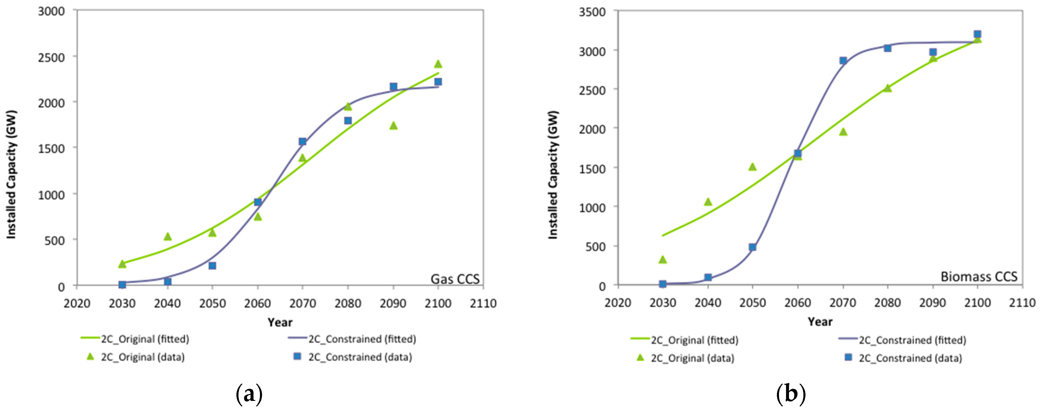
  • The second, named “2C_Constrained”, which is created in order to constrain the growth rate of key energy technologies which are observed to exceed the 20% limit as part of the “2C_Original” scenario, therefore making them somewhat at odds with the historical sustained growth rates observed by Iyer et al. [17] (Test 1 in Table 3). Such diffusion constraints are common in optimisation models to prevent unrealistic growth or dominance of any one technology. Since CCS is not yet deployed, a growth constraint is meaningless without first specifying what initial level of deployment is allowed in each region—a “seed” value of 1 GW of CCS in each region is therefore specified, reflecting that initial deployment is likely to see one or two large-scale CCS plants of the order 0.5–1 GW (i.e., commercial scale) in each region.
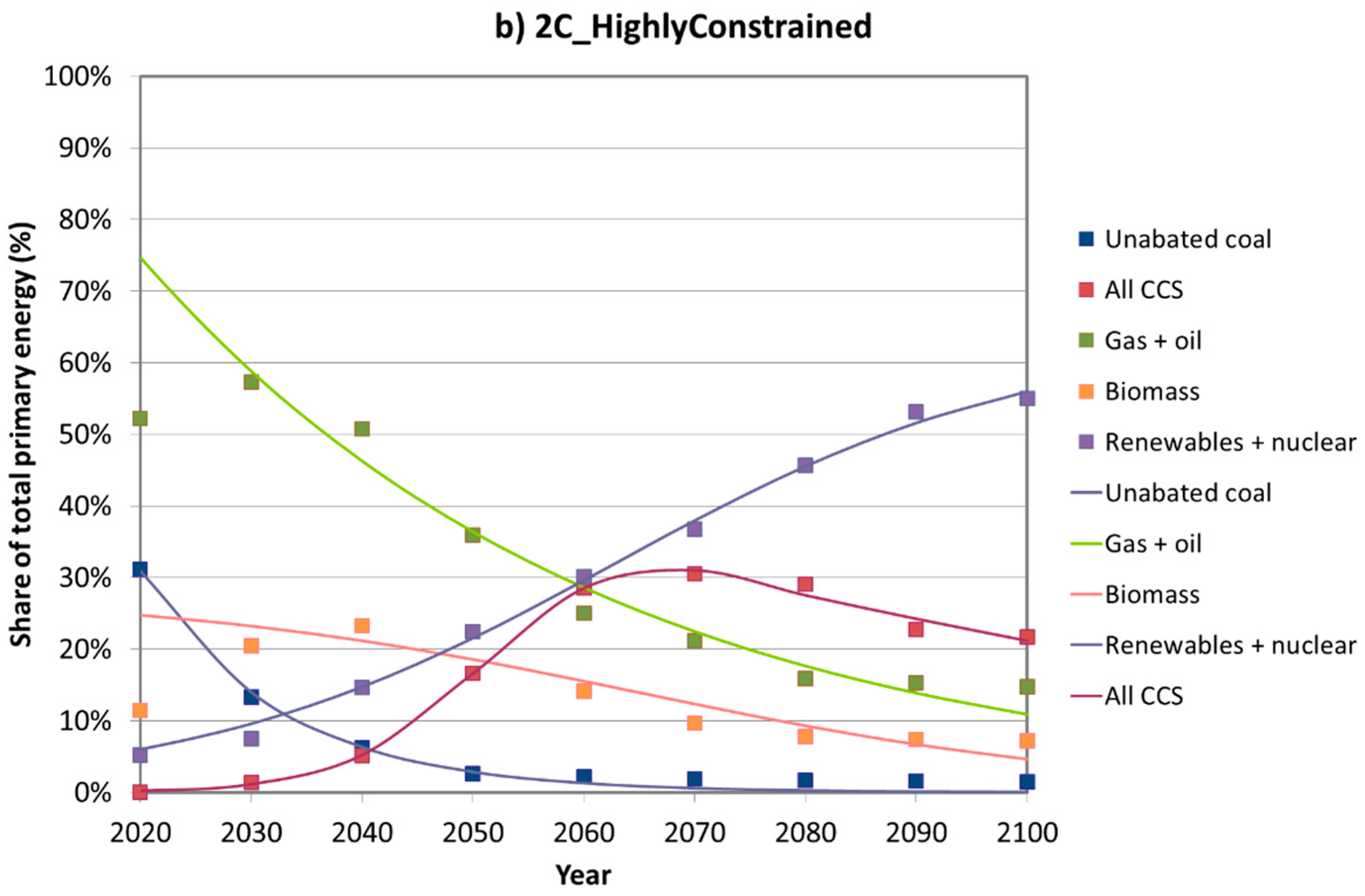
  • A third, named “2C_HighlyConstrained”, which is created in response to the application of all of the tests listed in Table 3 to the “2C_Constrained” scenario, and consideration of whether future low-carbon energy technology and energy resource patterns differ markedly from those patterns observed in the past. In particular, and as explained in greater detail in Section 5: the continued exponential growth of solar technologies beyond an initial growth phase is somewhat at odds with the past trends observed by Kramer and Haigh [21] (Test 5 in Table 3); the extent of wind deployment (in GW per EJ of total primary energy demand) in a given time duration, even with growth rates limited to 20% per annum, is significantly greater than for some other energy technologies as observed by Wilson et al. [23] (Test 3 in Table 3); and the rapidity of phase-out of coal as a primary energy resource is somewhat at odds with past trends as observed by Smil [11] and Gruebler [20] (Test 6 in Table 3).
For each of these scenarios, the implications of mitigation are assessed, in terms of the feasibility (i.e., whether the TIAM-Grantham model can provide a solution) and cost. Table 4 summarises the different features of the three scenarios. The third scenario, “2C_HighlyConstrained”, does not solve for the specified cumulative CO2 limit of 1340 GtCO2. The budget was increased in increments (of 50 GtCO2) until an analytical solution was found—in this case the minimum budget that can be achieved is 1540 GtCO2, which produces an estimated median warming of 2.1 °C rather than 2.0 °C as per the 1340 GtCO2 budget. This estimate is made by Met Office Hadley Centre on the basis of a simplifying assumption that the non-CO2 emissions and other climate forcing species are as per the “2C_Original” 1340 GtCO2 scenario. The full methodology for this analysis is outlined in AVOID 2 report WPC2a [3]. Also shown in Table 4 are the constraints imposed in response to applying the diagnostic tests listed in Table 3. These are explained in Section 5.

5. Results from Application of Diagnostic Tests

5.1. Summary of Diagnostic Test Results as Applied to the Low-Carbon Scenarios

Table 5 summarises the outcomes of applying the six tests to the three scenarios. As is clear from the table, the imposition of constraints on technology growth (and in the case of coal plants, a minimum level for their operation) brings the future low-carbon energy technology and resource transition patterns more closely into line with historical analogues as set out in the six tests described in Section 4, and Section 5.2, Section 5.3 and Section 5.4.
Adding these multiple constraints does, however, compromise the TIAM-Grantham model’s ability to solve for the stringent 1340 GtCO2 cumulative CO2 budget for the 21st century. Also of note is the more rapidly rising carbon price as the scenarios become more constrained. There is no contravention of Rogelj et al.’s [40] indicator of a CO2 price increase of greater than $1000/tCO2 per decade in the period to 2050 (which is equivalent to an oil price increase of $270/bbl, and assumed to be potentially economically disruptive), although this rate of increase is breached after 2070 in the 2C_HighlyConstrained scenario and after 2080 in the 2C_Constrained scenario. Countering this, it should be noted that by 2070 world economic output is projected to be more than 4 times larger than 2015 levels, according to the underlying socio-economic assumptions used in this modelling exercise. In terms of the impacts of the constraints on mitigation costs, the 2C_HighlyConstrained scenario almost doubles mitigation costs compared to the unconstrained 2C_Original scenario. Nevertheless, the costs still lie within recent ranges of mitigation cost estimates (for example the $12–120 trillion cumulative discounted cost of meeting a 450 ppm CO2e atmospheric stabilisation level of greenhouse gases reported in the 22nd Stanford Energy Modelling Forum exercise [41]).
In addition, this report focuses on feasibility through an assessment of rates of technology deployment of supply side technologies. Other dimensions of feasibility such as energy efficiency rates of improvement, negative emissions and stranded assets are not explicitly included here. However, Table 5 does include a figure for total CO2 captured throughout the 21st century by bio-energy with CCS (BECCS), given the importance of negative emissions technologies in meeting the 2 °C goal. As discussed in Section 5.3.1, the total CO2 captured in these scenarios is within the range of 2 °C-consistent scenarios within the IPCC’s fifth assessment report database, but significantly higher than the AVOID 2 upper estimate of 476 GtCO2 based on consideration of global land use constraints [42]. Whilst these limits are estimates, they nevertheless point towards the challenge posed by reliance on negative emissions in all of the scenarios analysed in this study.
The following subsections describe in greater detail how the assessment in Table 5 has been arrived at by considering each diagnostic test in turn.

5.2. How Rapidly Are Low Carbon Technologies Deployed?

5.2.1. Test 1: Assessing the Rates of Deployment of Low-Carbon Technologies

Table 6 shows the average annual growth rates (for each decade) in the 2C_Original scenario. The growth rates for nuclear, hydro and oil power are all less than the historical maximum growth rates for these technologies identified in Iyer et al. [17], which range from 7%–11% per year as shown in Table 7. Wind grows at a rate of 37% per year in the decade immediately following the start of global mitigation action (i.e., 2020–2030). In this decade, installed capacity of wind grows from 295 to over 6800 GW. To date, the highest average annual growth rates achieved for wind have been in Denmark at around 20% per annum over the period 1977–2008, with global rates averaging 19% per year over the period 2009–2013 [43]. CCS technologies show a rapid increase in the decade immediately after global co-ordinated mitigation action begins. Around 330 GW of Biomass CCS and 230 GW of Gas CCS is installed in this first decade, equivalent to an average annual growth rate of more than 70% (assuming a starting seed of 1 GW is allowed in the year when CCS is first deployed). It should be noted that this growth rate, stated with respect to a theoretical seed only, is not in itself infeasible. Nevertheless, as shown in Figure 5, imposing a growth constraint does result in a more credible pattern of CCS installed capacity growth.
In the 2C_Constrained scenario where CCS, solar and wind are constrained to a maximum growth rate of 20%, wind hits this maximum in 2020–2030 and a more gradual decline in the growth rate (compared to the 2C_Original scenario) is observed thereafter. As a result of the constraint on wind, higher growth rates are observed for solar compared to the 2C_Original scenario, but these still do not exceed 20% per year. For CCS technologies, although the sudden ramp up observed in the 2C_Original scenario is prevented, a high growth rate of around 20% is sustained for three decades. It is important to note that these assessments have been applied to only one model and so are not indicative of technology growth rates in all mitigation scenarios. As such, a model inter-comparison would be useful in elucidating the range of technology deployment rates across models.

5.2.2. Test 2: Comparing Future Technology Deployment Rates with Historical Rates

Figure 3 shows the comparisons of future average absolute capacity additions for low-carbon energy technologies from Van der Zwaan et al. [14] as well as from the two constrained scenarios (2C_Constrained and 2C_HighlyConstrained) using the TIAM-Grantham model for this study. All of these scenarios represent global action towards a 2 °C target beginning in 2020, following a period of weak regional climate policies to 2020.
The 2C_Constrained scenario has very rapid absolute wind GW growth rates over both the 2010–2030 and 2030–2050 periods—significantly higher than the median values from Van der Zwaan et al., although broadly in line with the top-end values of about 110 GW per year in the period 2010–2030, and 400 GW per year in the period 2030–2050. By contrast, the 2C_HighlyConstrained scenario, with a much more stringent growth rate of 5% per annum on wind (as discussed in detail in Section 5.2.3) sees much lower wind growth rates, on average 20 GW per year in the period 2010–2030 (which compares closely to historical values) and 50 GW per year in the period 2030–2050.
There is no clear indication of future scenario feasibility or infeasibility from this analysis, although the lower growth rates observed in the 2C_HighlyConstrained scenario do match far more closely the orders of magnitude observed for historical deployment rates (i.e., 50 GW per year for coal, the dominant power generation technology historically). As discussed in the following Section 5.2.3, overall energy system size is critical when considering the feasibility of future scenarios with reference to the past.

5.2.3. Test 3: Examining the Extent-Duration Relationship for Power Generation Technologies

In order to account for the fact that the energy system as a whole will be larger in the future, which by extension will enable larger annual installed capacities of energy technologies than have been observed historically, Wilson et al. [23] investigate the relationship between the “extent” of technology deployment and the time taken to reach this extent. The extent K is the long-run saturation level of the technology, expressed as maximum cumulative installed capacity (normalised for system size by dividing capacity by total primary energy demand at the point where 50% of saturation is reached). The duration Δ t is the time in years for the installed capacity to increase from 10% to 90% of K . The values of K and Δ t are determined by fitting a logistic growth curve to the data for each technology.
Figure 4 shows the extent-duration relationship for the key low-carbon energy supply technologies in the 2C_Constrained scenario, as well as for historical energy supply technology growth as collated by Wilson et al. [23]. If all power generation technologies from the 2C_Constrained scenario are included, then the trend line representing the extent-duration relationship across these technologies is much less steep than that for historical power sector technology deployments, which implies that they are not deployed as quickly as past technologies when normalising for the increasing energy system size. If nuclear (an obvious outlier) is excluded, the trend line is much closer to the historical trend line. The only technology above the extent-duration slope is wind. By imposing a 5% constraint on annual wind growth (as is the case in the 2C_HighlyConstrained scenario), wind shifts to a higher duration value such that it is more in line with this empirically derived extent-duration relationship (this is represented by the orange cross in Figure 4). It is important to note that the small number of historical data points in the power generation sector make these basic insights indicative only. However, this analysis does highlight the importance of controlling for changes in the size of the energy system when making historical comparisons.

5.3. What Is the Pattern of Low-Carbon Technology Deployment?

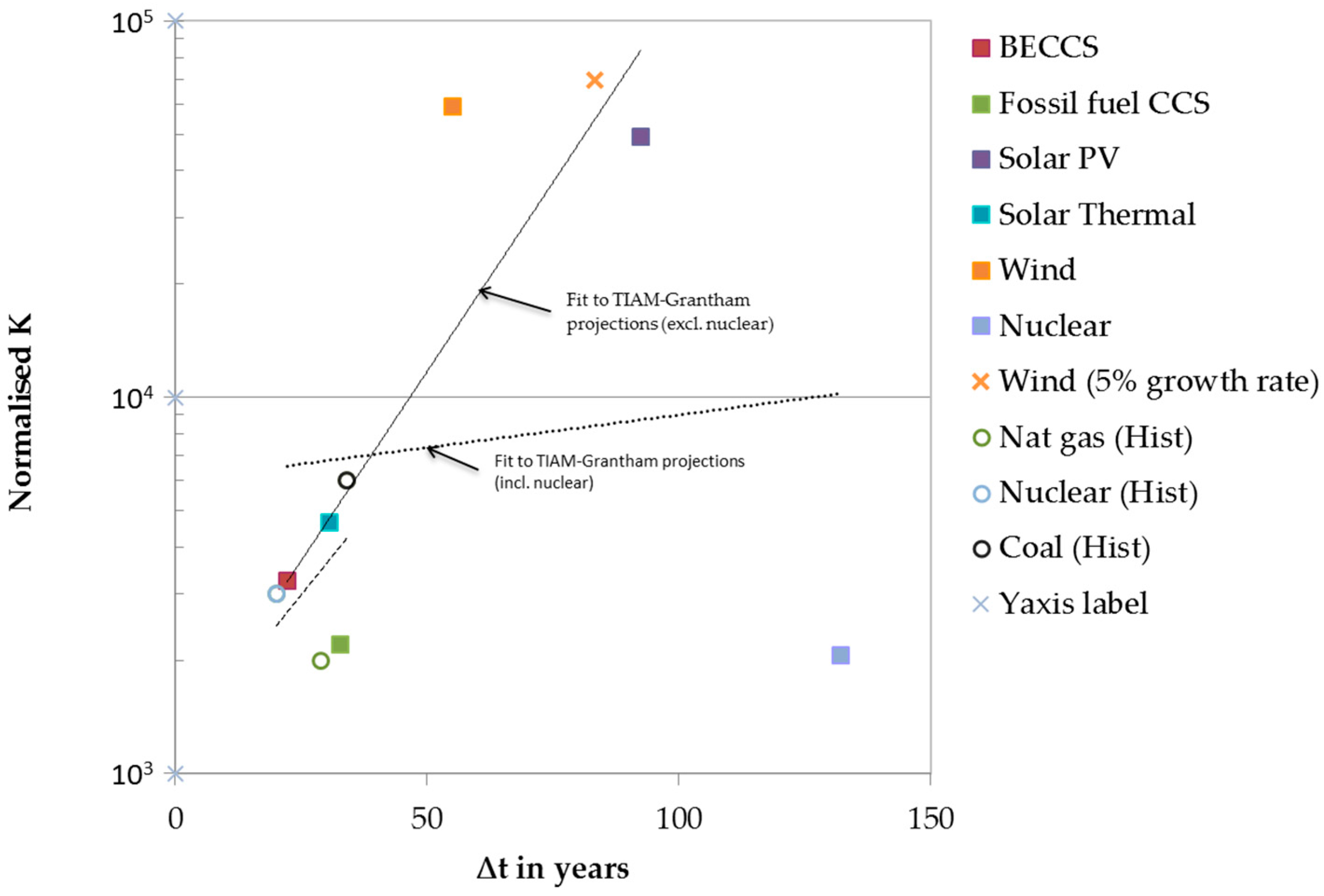
5.3.1. Test 4: Fitting Logistic Growth Curves to Power Generation Technology Deployment Levels

Besides looking at average growth rates and absolute values of installed capacity, a key outcome of the workshop described in Section 2 was that it is also important to consider the overall shape of the deployment curve. In particular, new technologies are likely, in reality, to ramp up slowly in their initial growth phase, as learning, supply chains, skills and expertise, finance, project management and business models are all established. The logistic curve is a widely accepted representation of the overall shape of the deployment curve. Using the approach outlined by Wilson et al. [23] (See Appendix C), logistic curves have been fitted to each technology in both scenarios.
Figure 5 compares the 2C_Original and 2C_Constrained scenarios for both (a) Gas CCS and (b) Biomass CCS, both of which see hundreds of GW deployed in the first decade (2020–2030) following the start of global mitigation action. This figure shows the impact of the 20% growth constraint on CCS technologies combined with a 1 GW seed value. This has the effect of lengthening the initial ‘tail’ during the early stages of the technology. Without this constraint in the 2C_Original scenario, a large leap in installed capacity from zero in 2020 to 230–330 GW in 2030 is observed. In addition, a clear levelling off is observed in the 2C_Constrained scenario as the technologies reach saturation, with gas CCS and biomass CCS reaching an extent value of 2220 GW and 3096 GW by 2100, respectively. As a result, the 2C_Constrained scenario represents an arguably more realistic deployment profile for these technologies than in the 2C_Original scenario, which means that they more closely follow an S-curve pattern as has been observed for a range of energy technologies to date [23,44].
The viability of deploying biomass with CCS, as a critical technology to achieve a 2 °C-consistent cumulative limit to 21st century CO2 emissions, requires further consideration beyond purely analysing its deployment rate. In the 2C_Constrained scenario, the total captured and sequestered CO2 from bio-energy with CCS is 805 GtCO2, compared to a median value of 610 GtCO2 captured in the 2 °C scenarios in the IPCC’s Fifth Assessment Report database.

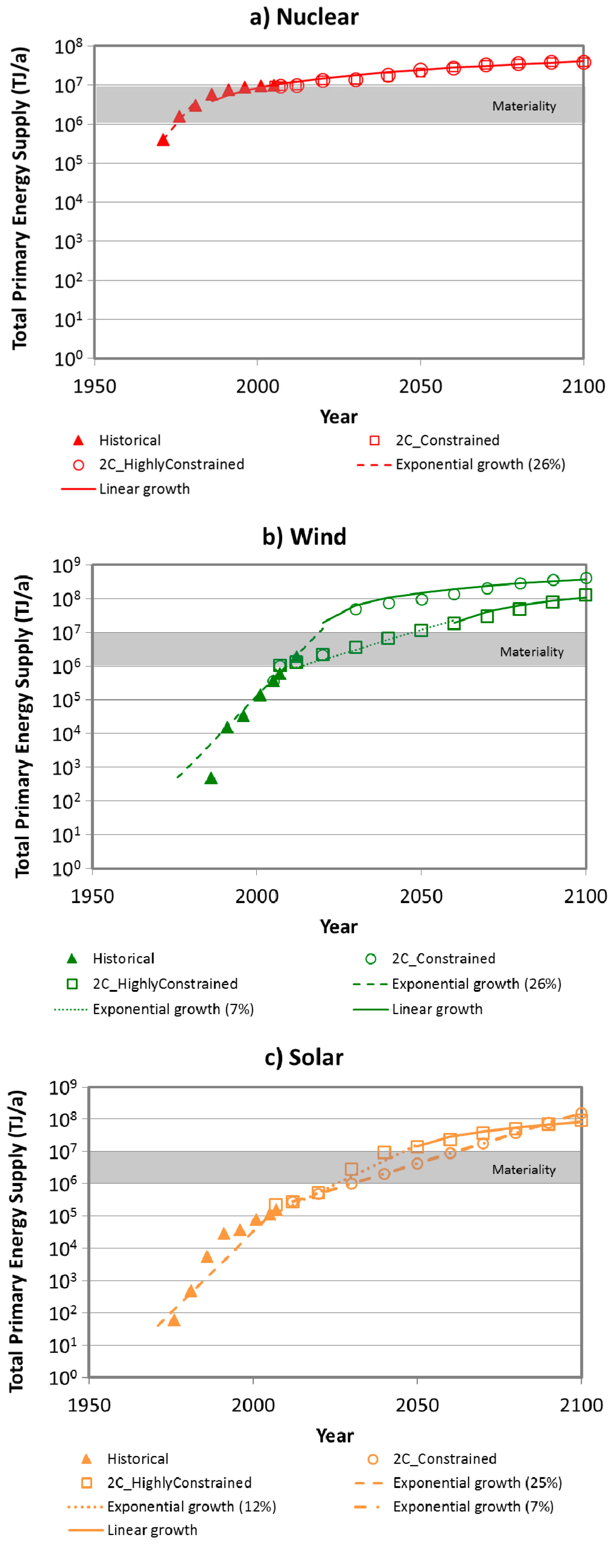
5.3.2. Test 5: Assessing Whether Future Technologies Break Kramer and Haigh’s Two Laws

Kramer and Haigh [21] also consider that it takes time for technologies to grow during the early stages and that there is a limit to how fast this growth can occur, largely because “it takes time to build the human and industrial capacity to achieve substantial deployment”. Based on analysis of historical energy transitions (as shown in Figure 6), they propose two “laws” of technology development:
  • Initially technologies go through a few decades of exponential growth, corresponding to a growth rate of approximately 26% per annum, until they reach “materiality” (i.e., supplying around 1% of the primary energy mix). Note that this appears to be faster than the fastest observed sustained capacity additions of around 20% per year as appear in Iyer et al [17], which have been used to constrain the technology capacity deployment rates in Section 5.2.1. Given that Iyer et al interpret their collated historical rates of technology growth to produce an upper bound of a 15% per year growth rate (which they deem high), we consider our 20% growth constraint to be a reasonable, though potentially conservative, assumption.
  • Beyond this, growth slows to linear growth typically at around 2%–4% per annum.
Figure 7 compares the growth of the total primary energy supply in the 2C_Constrained scenario and the 2C_HighlyConstrained scenario for three key technologies: (a) nuclear; (b) wind and (c) solar. Plotting total primary energy on a semi-log plot allows the transition between exponential and linear growth phases to be clearly observed. Figure 7a shows a short period of exponential growth for nuclear technology as it approaches materiality in the 1990s. This growth period conforms to the Kramer and Haigh [21] growth rate of 26% per annum. Once materiality is reached, nuclear transitions into a long period of linear growth, which continues out to 2100. This trend is observed for both the 2C_Constrained and the 2C_HighlyConstrained scenarios. In the 2C_Constrained scenario, Wind also shows a clear initial stage of exponential growth at 26% per annum as shown in Figure 7b. Soon after materiality is reached, wind transitions into a period of linear growth. The pattern observed for solar is shown in Figure 7c. Following a period of exponential growth at around 26%, exponential growth continues but at a rate of around 7% per annum. This stage continues well beyond materiality and a period of linear growth is not observed before 2100.
The more stringent constraints imposed in the 2C_HighlyConstrained scenario (specifically a 5% per annum annual growth limit on wind, and a 4% annual growth limit on solar after 2040) result in growth rates of these energy resources which are more in line with the laws outlined by Kramer and Haigh [21]. As shown in Figure 7b, in the 2C_HighlyConstrained scenario, wind growth slows once materiality has been reached and it transitions to a period of linear growth soon after. Similarly, Figure 7c shows that with a 4% growth rate imposed on solar after 2040 (the maximum rate in the range of Kramer and Haigh’s [21] post-materiality phase), solar also transitions to a period of linear growth soon after materiality is reached. Note that, in the 2C_HighlyConstrained scenario, solar PV has more of a role to play because of other constraints imposed (principally on wind) to go from constrained to highly constrained.

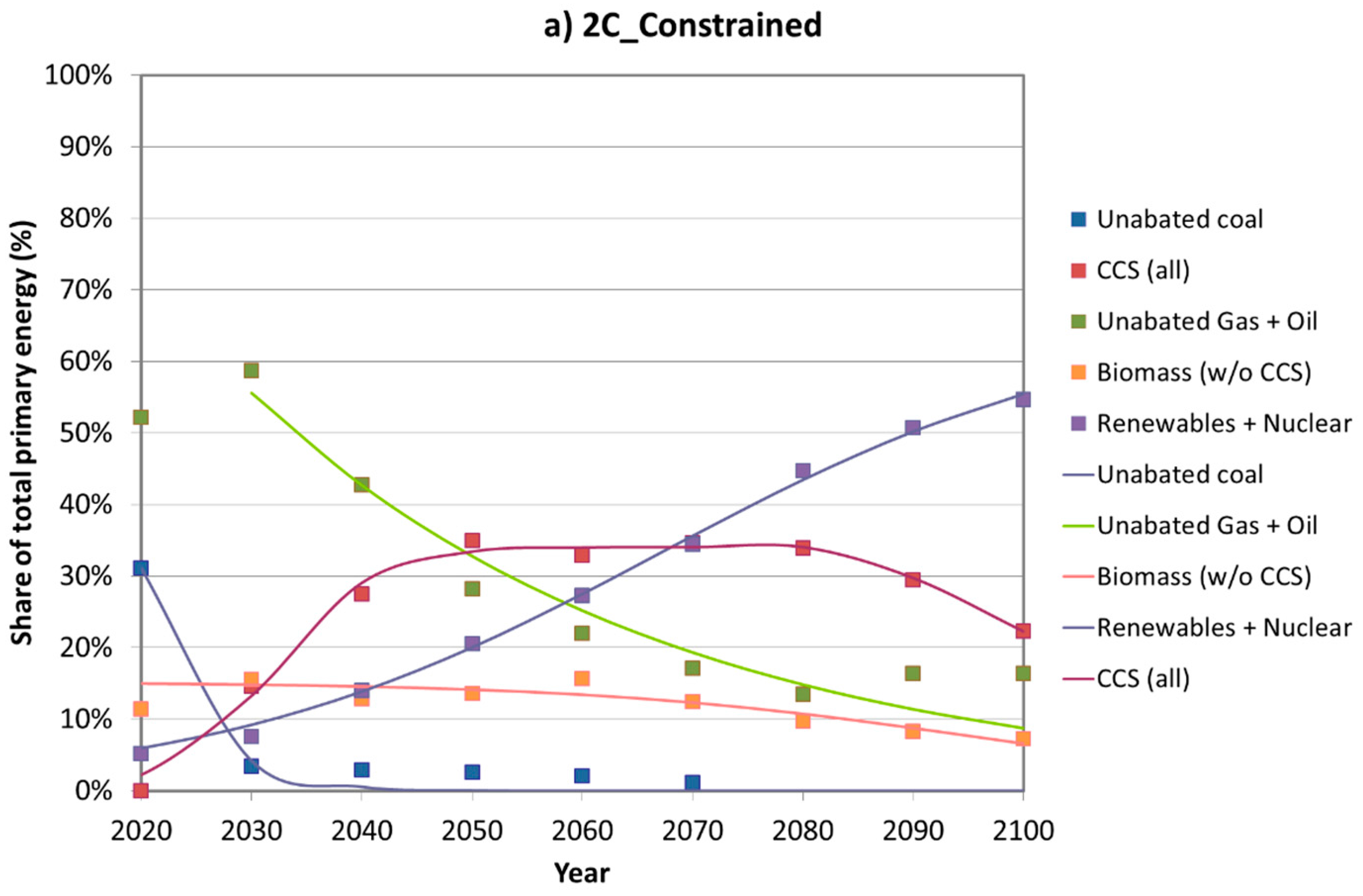
5.4. What Is the Rate of Transition between Primary Energy Resources?

Test 6: Assessing the Time Taken for Primary Energy Resource Shares to Rise and Fall

Figure 8a shows the share of total primary energy by fuel for the 2C_Constrained scenario. The data points indicate actual data from the model projections and the solid lines represent a fit to this data using a multiple logistic substitution model following the method outlined by Wilson and Gruebler [45]. Most noticeable is the speed at which coal is replaced with other energy sources. In the 2C_Constrained scenario a reduction in unabated coal from around 30% to less than 5% of global primary energy is observed in just one decade. Some of this is owing to coal being replaced with gas. Gas increases from 25% to 44% in the same time period. Much of the unabated coal is phased out, to be replaced with CCS technology which rises to around 30% by 2060. Unabated gas and oil are slowly phased out over the century to be ultimately replaced by renewables and nuclear. Biomass without CCS also declines in favour of BECCS technology.
As a result of the extremely rapid phase-out of coal, a minimum utilisation constraint has been placed on unabated coal-fired power stations, as explained in Section 4. This sees newly constructed coal plants maintain a 70% minimum capacity factor, and existing plants a 50% factor. As a result, the decline of unabated coal is slower, occurring over 4 decades as opposed to just one decade as per the 2C_Original scenario.
Table 8 shows the time Δt for each energy resource to increase from 10% to 90% of total primary energy share, for the projected scenarios and also for historical energy transitions (from Gruebler [20]). The Δt values for the phasing out of gas, oil and biomass and for the phasing in of renewables and nuclear are sufficiently long to not be considered infeasible given historical energy transitions. An exception is the decline phase for coal in the 2C_Constrained scenario, which is only 17 years. By forcing coal plants to remain online with a relatively high capacity factor, as in the 2C_HighlyConstrained scenario, this is increased to 34 years—still clearly challenging given the rather longer Δt periods for historical transitions. The Δt for CCS of 44–77 years is also short compared to historical global values, which highlights the challenge of deploying CCS when viewed from this perspective.

6. Implications and Conclusions

Historical energy transitions, at both the energy resource and energy technology levels, provide potentially useful insights to inform the plausibility of future low-carbon scenarios. Over recent years a body of literature has emerged which seeks to compare future low-carbon scenarios with patterns and trends of energy transitions from history, in order to gain insights into the level of challenge posed by these futures. This study, drawing from and building on this literature, as well as the views of experts in the fields of energy systems modelling and energy transitions, applies a set of diagnostic tests to a selected low-carbon scenario aimed at achieving a 2 °C limit to global warming by 2100, in order to assess how its energy technology and primary energy resource patterns compare with history.
By applying growth and other technology constraints to this scenario in response to these diagnostics, two further low-carbon scenarios are created—the first with key energy supply technology growth rates constrained to 20% per annum, reflecting the higher end of previous energy and pollution control technology growth rates, and the second with additional growth constraints to wind and solar, as well as the specification of a minimum usage level of unabated coal generation plants. The second scenario, with its range of constraints, shows future primary energy and energy technology transition patterns which match historical experience reasonably well. However, with these constraints the energy systems model used to produce the low-carbon scenarios can no longer solve, indicating that the constraints are possibly too binding to allow the realisation of a 2 °C target to be met with 50% likelihood. The minimum median 2100 temperature change that can be reached is about 2.1 °C, although at more than twice the cumulative cost of the unconstrained scenario.
Whilst these tests produce valuable insights into the challenges to be overcome in achieving a low-carbon transition, a number of caveats to the analysis must be highlighted, which provide avenues for further research. The first is that the analysis of historical transition rates can only be a rough guide to the future, since there can be (and have been) very rapid short-term growth rates in individual technologies and energy resources in specific regions. Although various barriers to the uptake of technologies exist, as listed in Section 2.3, there is no fundamental reason (e.g., a physical resource limitation) why such rapid growth cannot be reproduced at larger scales and longer time periods with sufficient effort from governments, businesses and other stakeholders to overcome these barriers. The second is that a number of contextual factors are not captured in the energy systems models such as the TIAM-Grantham model used in this analysis—these models can only directly represent technological (and in some cases and to a limited extent) economic systems, not social or political systems. Such factors will be critical to determining the real-world drivers and barriers to future energy transitions. Hence, comparing the future projected scenarios with past trends overlooks a number of elements which could make the future context in which a low-carbon transition occurs very different from past circumstances which have driven historical transitions. Thirdly, the analysis, in building on recent literature, focuses only on the energy supply side. Clearly future mitigation feasibility will also depend heavily on energy efficiency improvements and the rate of penetration of low-carbon energy demand technologies into the major end-use sectors (transport, buildings and industrial manufacturing). Further analysis should include the assessment of demand side technology transitions. Finally, it is also necessary to consider the physical supply limits to key low-carbon energy technologies. In many cases (as with TIAM-Grantham) the integrated assessment models contain such limits, for example on total available fossil, uranium, wind and other resources. However, a more explicit framing of low-carbon transition assessments in the context of all potential constraints (including skills, essential rare earth elements, land, water and other resources) is an emerging field.
These caveats aside, what is clear from this analysis is that low-carbon transitions will require rates of energy supply technology deployment and rates of declines in fossil fuels which are unprecedented, if the 2 °C goal is to be achieved.

Supplementary Materials

Responses to the post-workshop questionnaire are provided as supplementary material. These are available online at www.mdpi.com/1996-1073/10/1/116/s1.

Acknowledgments

This work was undertaken as part of the AVOID 2 research programme funded by the UK Government under contract reference number 1104872. Further details of AVOID 2 are available at www.avoid.uk.net. (Open access funds details to be added when finalized—so far we have applied to Imperial College’s central funds for Open Access.). The authors would also like to acknowledge the contribution of Charlie Wilson from the Tyndall Centre for Climate Change Research who reviewed an early draft of this paper as part of the AVOID 2 programme.

Author Contributions

Ajay Gambhir and Rebecca Thomas conducted the literature review and ran the energy transitions workshop; Tamaryn Napp and Ajay Gambhir designed the diagnostic tests; Tamaryn Napp ran the TIAM model and analysed the model outputs with assistance and advice from Ajay Gambhir and Adam Hawkes; Dan Bernie ran the climate models to calculate associated temperature rise; Tamaryn Napp wrote the bulk of the paper with significant contributions from Ajay Gambhir; Jason Lowe was chief scientist for the AVOID 2 programme of which the research presented in this paper formed a part.

Conflicts of Interest

The authors declare no conflict of interest.

Appendix A. Note on the AVOID 2 Energy Transitions Workshop (16 October 2014, Imperial College London)

Appendix A.1. Session 1 Discussion Points:

  • Speed of technology take-up depends on the technology in question:
    For example, CCS is a bulky, complex technology, which involves new infrastructure, project management, business models and significant financing.
    By contrast, solar PV is modular, can be deployed at small-scale and can be less capital intensive.
    Electric vehicles require only a change in drivetrain to existing car designs. This, combined with relatively short vehicle lifetimes, means that rapid take-up rates of EVs are plausible. 12% of new cars sold in Norway are EVs, incentivised by subsidies and other softer measures such as access to bus lanes, higher purchase taxes on conventional vehicles (i.e., very targeted policies to affect purchase behaviours)
    However, unless the grid is highly decarbonised, such as that in Norway, the well to wheel emissions for electric cars are similar to those of efficient internal combustion vehicles (this would be the case for the UK). Consequently, for there to be significant benefit in a rapid uptake of electric vehicles, over and above a stringent emissions standard for IC engine cars, not only would the grid need to have significantly more capacity, but it would need to be very low carbon.
  • Speed of technology take-up depends on the tail before rapid take-off:
    Solar PV has had a very long tail of development and deployment leading to the recent significant increase in cumulative capacity. The same is true of wind.
  • Success of a technology also depends on whether it can have benefits beyond just carbon reductions:
    These might be for example whether it can gain a wide variety of new applications (as with General Purpose Technologies such as the steam engine, though in practice it is not possible to tell in advance which technologies or combinations of technologies will become GPTs)
    Alternatively, it may have significant co-benefits (e.g., reduced air pollution, energy security) which make it attractive from a private/national perspective in the earlier stages of deployment, without considering its global social (climate) benefit.
  • Businesses’ considerations will be critical in determining technology take-up rates:
    Businesses (e.g., refining) consider the time it takes to deploy technologies as well as the potential for cost reductions as technologies get deployed.
    In addition, rates of return for investment in new technologies are technology- and region-specific, reflecting these context-specific investment risks. The key to many business investment decisions is not so much technology-specific hurdle rates, but the forgone returns from alternative investments.
    The response of business is itself cultural specific. Anglo-Saxon nations tend towards high discount rates and legal frameworks that favour share-holder return. There are significantly different models in other parts of the world; for example share-ownership and short-termism are less dominant in Germany.
    Businesses also operate within a legal framework, so the use of emissions standards and other forms of regulation can rapidly change the business environment (though it is probably wise that politicians refrain from picking technology winners, and instead simply set the regulatory and emission standard framework within which industry must deliver/operate.
  • Technology take-up rates cannot be considered outside of the social and political context:
    We are deeply locked-in to the technologies, institutions and norms of a fossil fuel energy system.
    Any radical replacement of fossil technologies will see significant destabilisation of this status quo.
    There needs to be a process of path creation for new and existing players in the energy system, in order to provide a transition path to a low-carbon system. An example of context-specific conditions is the rapid switch from town to natural gas (an established industry already looking for new opportunities, the specific era of governance with firms working closely with government) which saw very high levels of stranded assets but nonetheless succeeded.
    Particular policies which drive forward the technologies will be critical.
    End-use technologies have very rapid turnover rates (typically less than 10 years for cars, fridges, toasters etc.) and are therefore an exception to the issue of ‘lock-in’. Emission standards here could see very rapid transitions away from current levels of fossil fuel consumption—provided rebound issues were addressed.
  • The “marginal economics” nature of energy-technology models may limit their usefulness in projecting fundamental energy system and energy demand changes.

Appendix A.2. Session 2 Discussion Points

  • We are rapidly consuming our available carbon budget for the 21st century.
  • A view was given that we cannot build low-carbon technology supply fast enough to make a significant impact on the current rate of emissions growth for many years to come, which highlights the importance of demand reduction.
  • Consideration of requisite rates of decarbonisation needs to be clear about the probability of remaining below 2C.
  • Requisite rates should not account for negative emissions technologies in all scenarios—exploring scenarios with and without negative emissions is better.
    However, if models represent bioenergy and CCS, then why not BECCS—perhaps better to consider limiting bioenergy and/or CCS as well/instead.
    One opposing argument is that there are a number of low-carbon technologies vying for bioenergy and the availability of biomass across all technologies needs to be considered.
  • Energy demand reduction provides a feasible opportunity to make significant emissions cuts in the short term, but needs very effective policies.
    Example given of setting effective vehicle emission standards which could reduce emissions (considering turnover rates and some early scrappage) by 50% in 10 years.
  • Should be more explicit consideration and explanation of underlying economic growth pathways that relate to each mitigation scenario
    The Shared Socioeconomic Pathways (SSP) work is beginning to address this point, since to date the socio-economic storyline for each Representative Concentration Pathway has been different, but the SSP initiative will allow matching of RCPs to different SSPs.
  • Feasibility of decarbonisation rates cannot be considered without first considering what can be achieved in each sector by each technology, measure and policy.
  • Many integrated assessment models do not have detailed representations of energy end-use technologies, and none have detailed representations of energy usage behaviour and detailed take-up patterns for end-use technologies. These limitations should be carefully considered in low-carbon scenarios.
  • Low cost or even cost-saving energy demand reduction measures can help buy time for the implementation of low-carbon technologies. In addition, demand side is just as important as supply to energy security.
  • With TIAM, which does have representation of energy demand technologies, it would be worthwhile considering what would happen in optimal scenarios when all cost-saving efficiencies are taken up, and in other scenarios where behaviour is not “optimal” in this narrow economic sense. A key question is defining how far real-world behaviour would deviate from this cost-optimality.
  • Integrated assessment models mostly do not consider feedbacks from future energy systems to economic systems (other than through a marginal demand response as the price of energy rises with increased low-carbon technology share). In general no climate feedback to the economy’s output is modelled (although some projects are beginning to look at this—HELIX being one).
  • It is worthwhile considering the impact of removing key technologies (not just BECCS) from the portfolio to assess feasibility and cost of low-carbon scenarios.

Appendix A.3. Session 3 Discussion Points

Summary of discussion on wind and solar deployment feasibility:
  • Barriers:
    Wind at scale will require a lot bulkier capital investments;
    Wind not viable at small (household) scale and will face land constraints;
    Wind technology more mature, less room for cost reduction;
    Grid connections to wind could be a constraint;
    For solar, possible supply chain and material constraints need to be considered;
    Centralised generators do not favour decentralised technologies like solar.
  • Overcoming barriers:
    Weather-based energy pricing to support solar and wind intermittency;
    Appliance design could be modified to handle intermittent generation;
    Smart systems with storage (e.g., from EVs & domestic thermal storage) would also help enable solar and wind;
    Specific policies have been successful in nurturing these technologies to rapid growth;
  • Overall, none of the models’ rates of technology growth seem fundamentally infeasible, and solar in particular could grow faster, sooner.
Summary of discussion on energy intensity:
  • Large variations in base year figures noted between different models.
  • Difficult to unpick what causes energy intensity reductions in each sector:
    How much is structural (e.g., shift to less energy-intensive industry);
    How much is technological (e.g., shift form ICE to EVs in transport);
    How much is demand reduction (e.g., travel less by car, switch lights off more frequently).
  • Energy intensity is not a factor in itself to constrain, but the underlying factors need greater analysis.
  • Overall, none of the rates of intensity improvements looked particularly infeasible, but need to understand the underlying drivers to assess this more thoroughly. e.g., electrification of end-use sectors could see significant energy efficiency savings, but need to consider what is driving electrification and how effective this driver is.
Summary of discussion on nuclear and CCS:
  • Cannot consider the ramp-up rate of each technology by region in isolation, as supply chain capacity for a given technology can be considered a global resource, while the development of capacity (e.g., training engineers) in a given region probably implies trade-offs between technologies’ growth rates. Therefore need to consider what other technologies are being invested in globally and regionally, as these will compete for construction, skills, finance etc.
  • Scenarios do not consider small nuclear reactors—just GW-scale.
  • Overall, rapid post-2030 ramp-ups of nuclear and CCS look unrealistic unless there has been significant tooling up, investment in skills and infrastructure. Lead times for capital-intensive technologies such as this will be several years, potentially a decade—this must be accounted for.
  • LCA (life-cycle assessment) carbon emissions for CCS are likely to be above 80 g CO2/kWh—and possibly much higher (unless technologies change and upstream capture of fugitive emissions is achieved). This places the LCA emissions of CCS at 4 to 20 times greater than the LCA carbon emissions for renewables and nuclear technologies. As a consequence, with more electrification the relative role of CCS in the power systems of Annex I countries is highly constrained by the available carbon budgets. So CCS is a viable transition technology for non-Annex I countries but much less so for Annex I countries.
Final discussion points:
  • Modelling of this nature is not about predicting the future but more about identifying technology possibilities before considering how to support these technologies.
  • Modelling develops heuristics—it helps us understand the system; the actual results need to be treated with considerable caution and continually sense checked.
  • A number of considerations should be brought to bear when considering scenario feasibility:
    Technology costs and how these could develop with deployment (noting the considerable uncertainties around future costs);
    Technology co-benefits;
    Supply chain and material constraints;
    Trade-offs between technologies considering competition for skills, capital;
    Supporting technologies;
    Initial “tail” of deployment, including long lead-times for capital-intensive projects like CCS and nuclear;
    Policy effectiveness;
    Socio-political context accounting for lock-in to a fossil energy system.
  • The demand side technologies, measures and policies are critical in achieving rapid emissions reductions, in many cases at low or negative costs, so should be considered more thoroughly.
  • Important that models do not all “revert to a mean” so that there are no outliers—this may preclude important possible patterns of technology deployment (e.g., one technology showing significant dominance eventually). Against this, the massive increase in electricity generation as end-use sectors become electrified will probably require several different electricity generation technologies to be deployed.

Appendix B. Post-Workshop Questionnaire on Understanding the Feasibility of Energy System Transitions in Energy Technology Models

This appendix presents the post-workshop questionnaire which was sent out to workshop attendees. Detailed responses to the questionnaire are provided in the supplementary material.

Introduction

This questionnaire is a follow-up to the discussion at the AVOID 2 energy transitions workshop held at Imperial College on 16 October 2014. It consists of nine questions in four different sections. Responses, in addition to notes from the workshop, will be used in forming views on mitigation scenarios developed in the AVOID 2 work programme. Responses may also form the basis of published analysis on energy and climate experts’ views on energy transition feasibility. Please note that all responses will remain anonymised in any published reports.
Please enter your name here: ________________________________
Level of knowledge in energy and technology transitions
1.
Please state your level of expertise in energy transitions research (High, Medium, Low)
2.
Please state your level of expertise in energy modelling (High, Medium, Low)
General views on how to critically assess technology take-up rates
3.
At the AVOID 2 workshop on energy transitions, a number of factors were discussed as potentially important in considering the real-world feasibility of different technology take-up rates. Which four of these factors are most critical (ranked 1: most critical, to 4) when undertaking a feasibility assessment of technology take-up rates?
  • Degree to which there has been a ramp-up “tail” period before rapid deployment
  • Co-benefits of the technology beyond low-carbon
  • Cost reduction potential of technology
  • Lead-time to build and deploy technology
  • Availability of complementary or supporting technologies/infrastructure
  • Deployment of other low-carbon technologies which compete for resources
  • Capital-intensiveness of technology
  • Lifetime of technology
4.
On a scale of 1 (not at all useful) to 5 (very useful), how useful is it to consider (either in absolute terms, as % growth rates, or as shares of total technology capacity) the historical take-up rates of energy technologies when assessing the feasibility of particular low-carbon energy technology take-up rates in future mitigation scenarios? Please explain your answer.
5.
In addition to factors (a–h) in question 1 above, as well as historical take-up rates of energy technologies, are there any other factors which should be considered when assessing the feasibility of technology take-up rates in mitigation scenarios?
General views on how to critically assess energy system changes in energy technology models
6.
Thinking beyond specific technology take-up rates and to broader energy systems, how useful (on a scale of 1: not at all useful, to 5: very useful) are the following methods to assess the feasibility of achieving future mitigation scenarios?
  • Some analysis has considered the time taken for different energy sources to attain particular shares of total primary energy supply (either globally or regionally), as a guide to how rapidly low-carbon energy sources might attain given shares in the future.
  • There has been some assessment of feasibility based on whether the mitigation scenarios involve a rapid increase in carbon prices over a short time period.
  • Feasibility assessment has also considered whether absolute carbon prices reach particularly high levels.
7.
Which other metrics could be useful in assessing the feasibility of achieving future energy systems in mitigation scenarios?
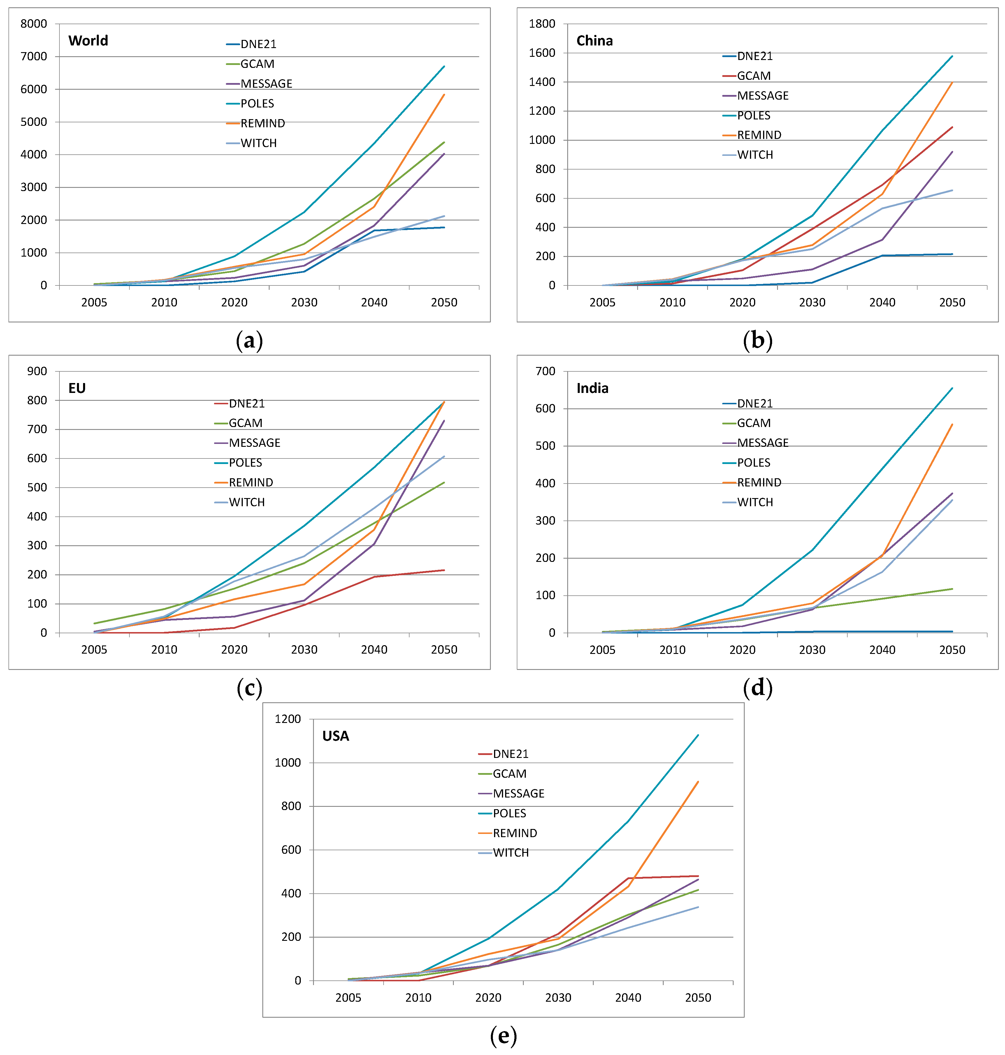
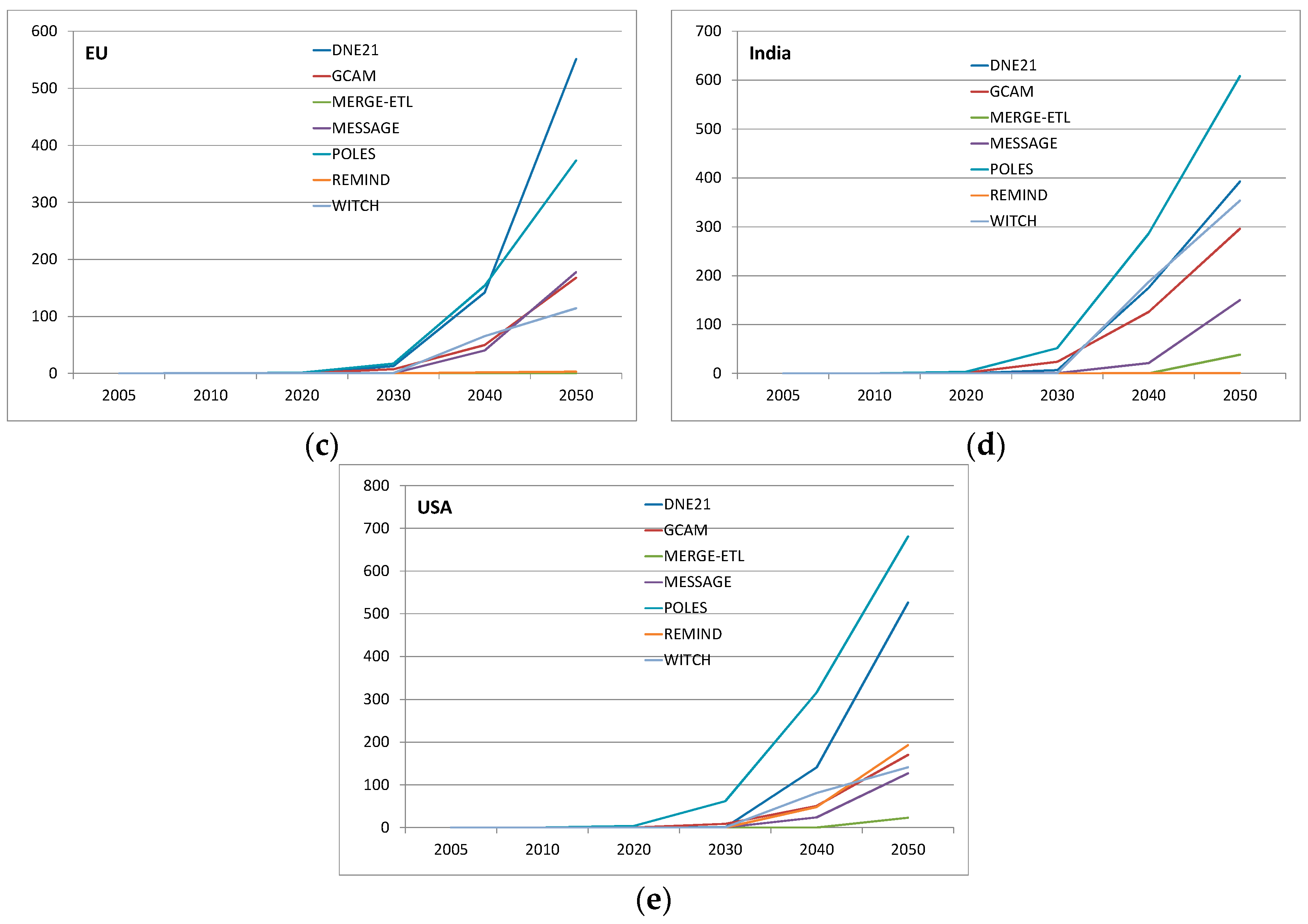
Views on specific technology take-up rates
8.
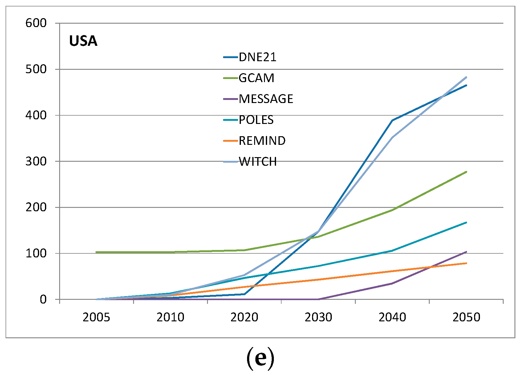
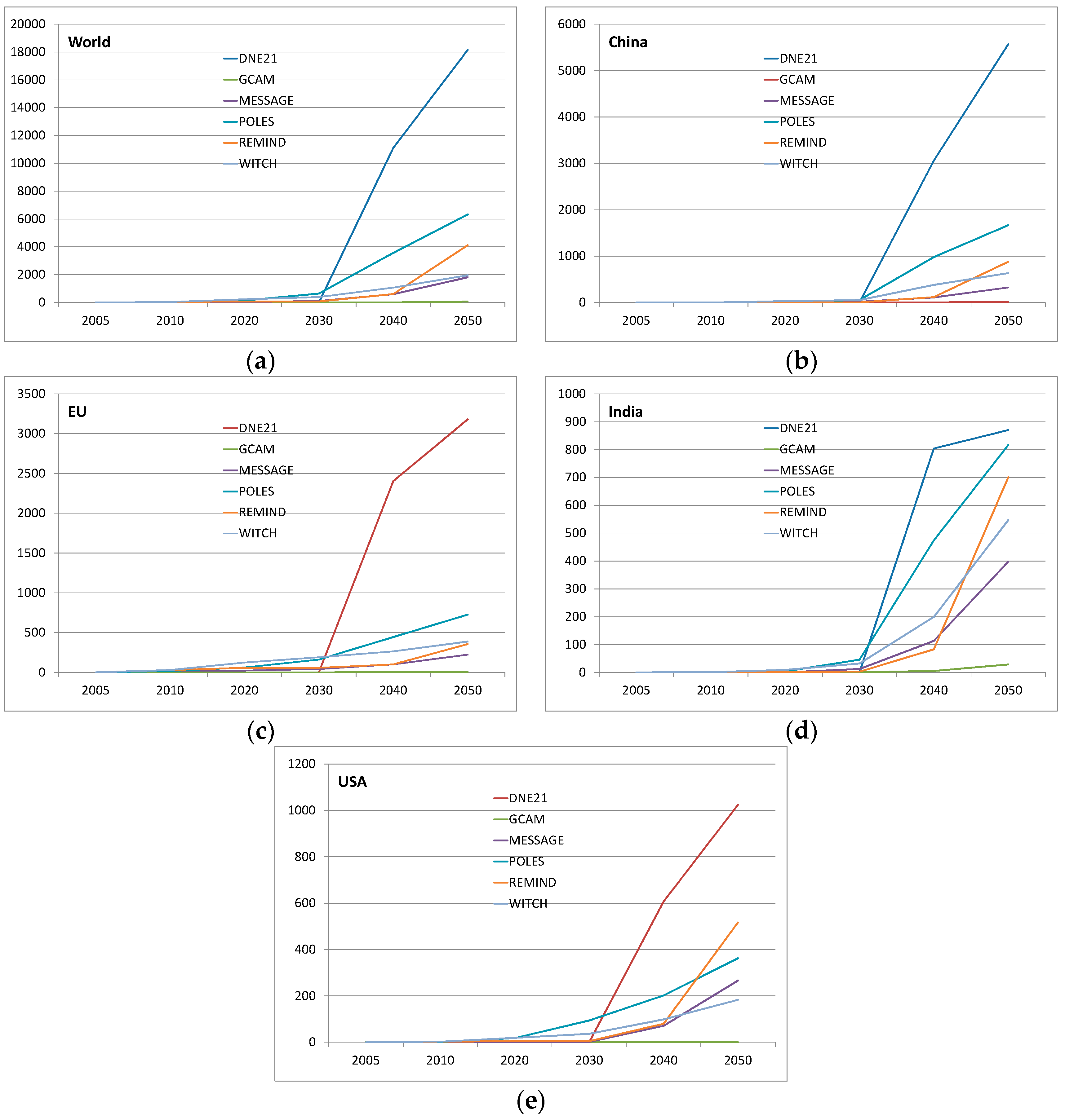
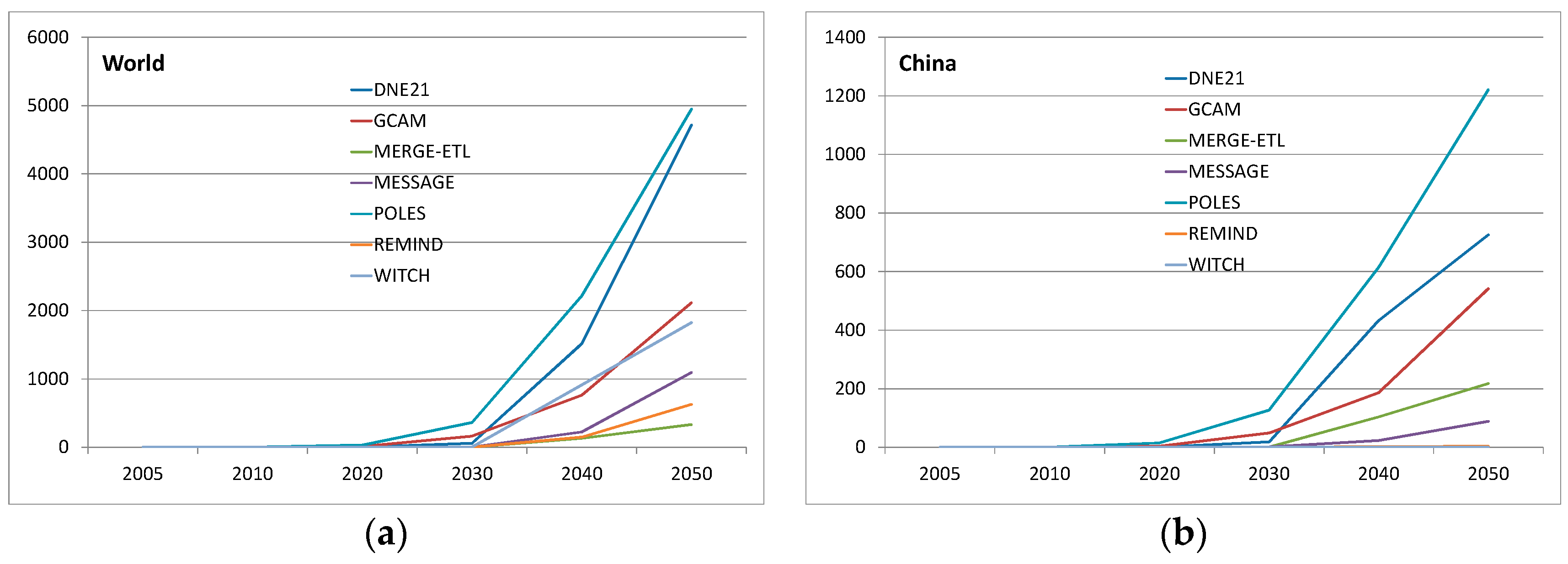
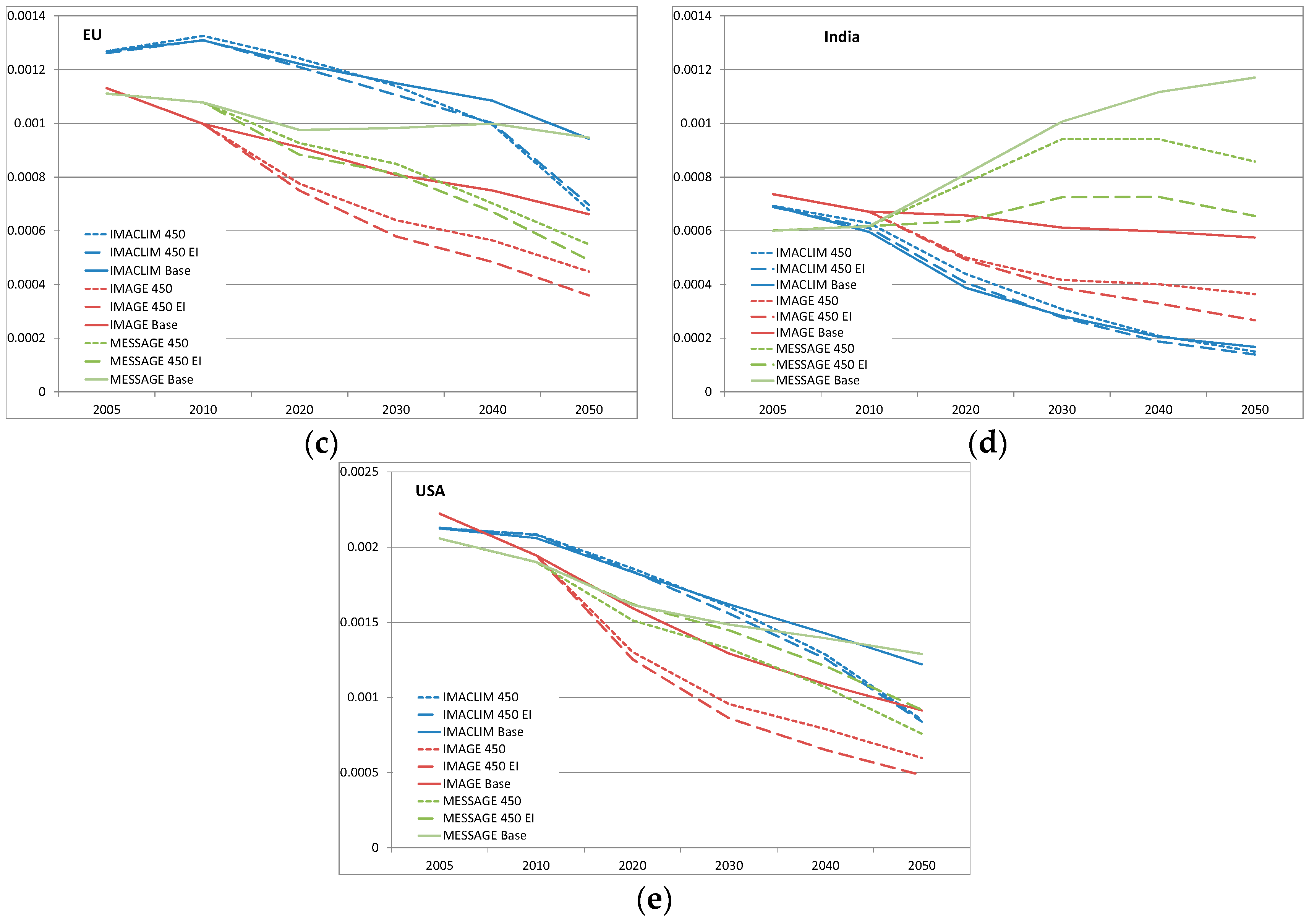
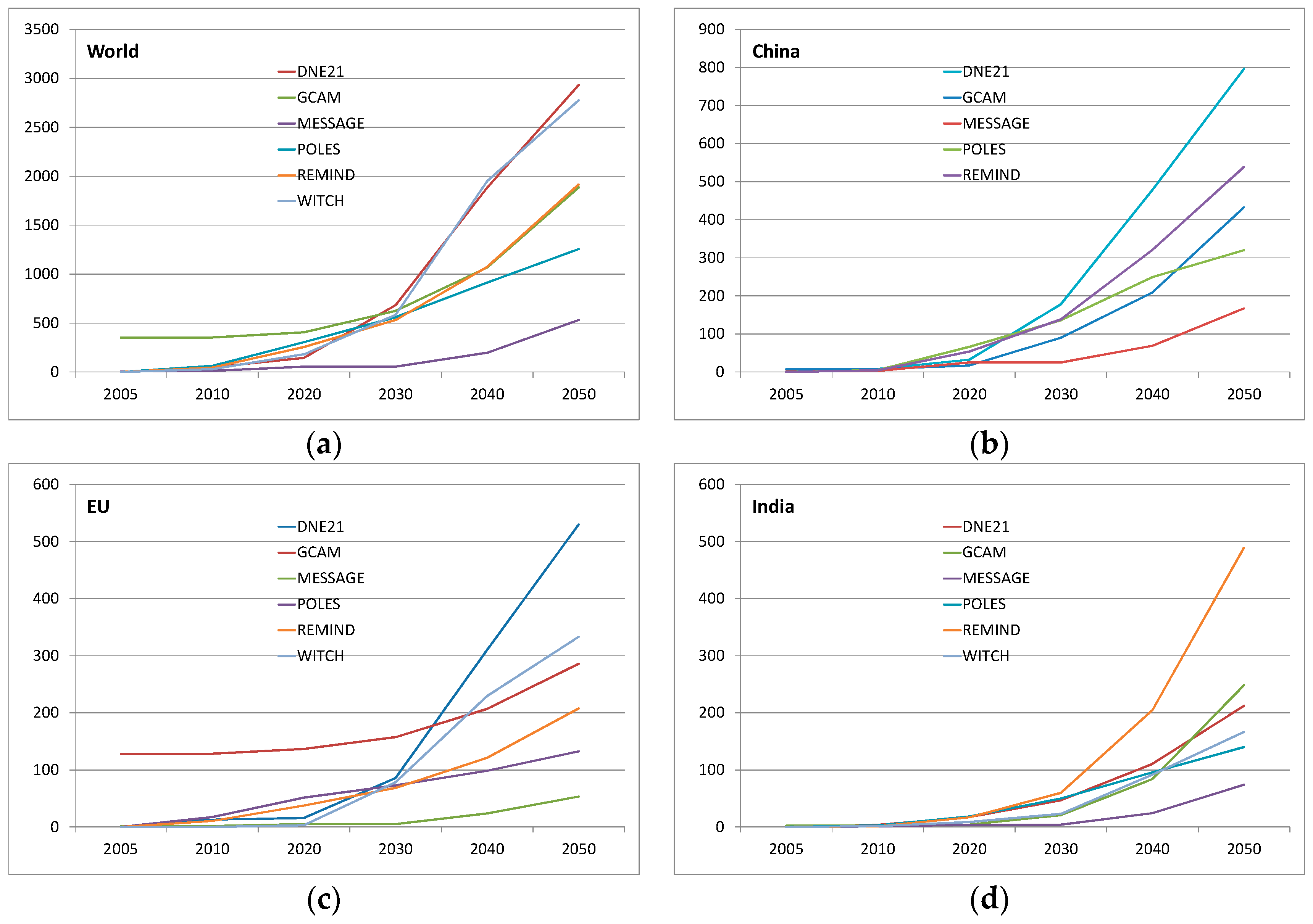
The following figures show the cumulative capacity deployed in different regions, using different energy-technology models, in the Ampere study (one of the major inter-model comparison projects to be included in the IPCC’s fifth assessment report). Underneath each figure the average annual growth rate over the period 2030–2050 is given (except for CCS, which is 2040–2050, since in many models no CCS is deployed by 2030). The particular scenario details are:
  • “weak” country/region action in line with the lower (less ambitious) end of Cancun pledges to 2030, followed by global mitigation action aimed at achieving a 450 ppm concentration of GHGs;
  • no specific details on technology R&D and planning before global mitigation action begins, though it may reasonably be assumed that current policies and R&D and demonstration programmes (e.g., for CCS) continue.
Please say, for each of the following technologies, which deployment rates (if any) look unrealistic and why, considering both World and Regional deployment patterns.
Figure B1. Inter-model comparison of installed capacity (GW) for nuclear in (a) World (2030–2050 growth rate = 4%–12% p.a.); (b) China (2030–2050 growth rate = 4%–12% p.a.); (c) The EU (2030–2050 growth rate = 3%–13% p.a.); (d) India (2030–2050 growth rate = 5%–13% p.a.) and (e) USA (2030–2050 growth rate = 3%–6% p.a.).
Energies 10 00116 g009aEnergies 10 00116 g009b
Figure B2. Inter-model comparison of installed capacity (GW) for solar PV in (a) World (2030–2050 growth rate = 8%–22% p.a.); (b) China (2030–2050 growth rate = 13%–35% p.a.); (c) The EU (2030–2050 growth rate = 4%–10% p.a.); (d) India (2030–2050 growth rate = 15%–22% p.a.) and (e) USA (2030–2050 growth rate = 3%–30% p.a.)
Energies 10 00116 g010
Figure B3. Inter-model comparison of installed capacity (GW) for wind (offshore and onshore) in (a) World (2030–2050 growth rate = 5%–10% p.a.); (b) China (2030–2050 growth rate = 5%–13% p.a.); (c) The EU (2030–2050 growth rate = 4%–10% p.a.); (d) India (2030–2050 growth rate = 0–10% p.a.) and (e) USA (2030–2050 growth rate = 4%–8% p.a.).
Energies 10 00116 g011
Figure B4. Inter-model comparison of installed capacity (GW) for coal and gas CC in (a) World (2030–2050 growth rate = 7%–17% p.a.); (b) China (2030–2050 growth rate = 0–15% p.a.); (c) The EU (2030–2050 growth rate = 6%–15% p.a.); (d) India (2030–2050 growth rate = 6%–22% p.a.) and (e) USA (2030–2050 growth rate = 6%–18% p.a.).
Energies 10 00116 g012aEnergies 10 00116 g012b
9.
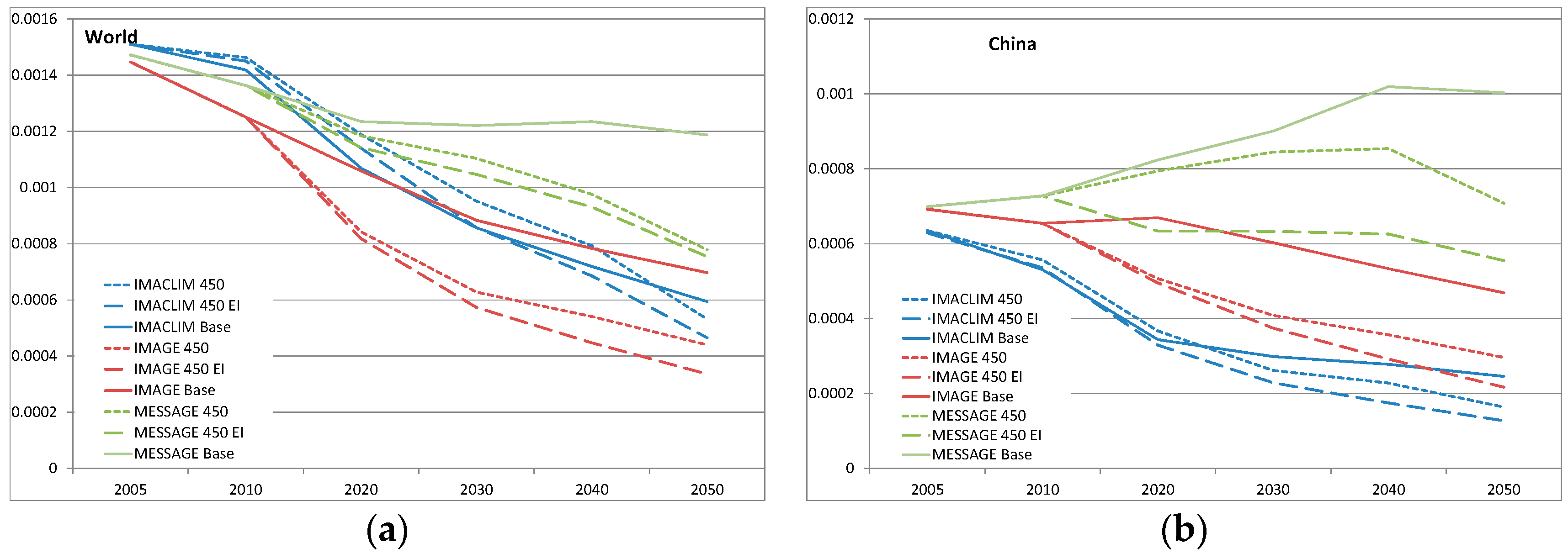
Figure B5 shows the change in energy intensity in the transport sector in different models from the Ampere study, in:
  • a baseline scenario;
  • a 450ppm scenario with immediate action (starting in 2010) and;
  • a 450ppm scenario with immediate action and higher energy intensity improvements.
Please say which energy intensity rates of change (if any) look unrealistic and why, considering both World and Regional deployment patterns.
Figure B5. Inter-model comparison of the change in energy intensity in the transport sector in (a) World (Annual rate of energy intensity improvement: 2005–2010 = 2%, 2010–2050 = 1% to 3%); (b) China (Annual rate of energy intensity improvement: 2005–2010 = 1%, 2010–2050 = −1%–4%); (c) The EU (Annual rate of energy intensity improvement: 2005–2010 = 1%, 2010–2050 = −2%–4%); (d) India (Annual rate of energy intensity improvement: 2005–2010 = 1%, 2010–2050 = 0.3%–2.5%) and (e) USA (Annual rate of energy intensity improvement: 2005–2010 = 2%, 2010–2050 = 1%–3%).
Energies 10 00116 g013aEnergies 10 00116 g013b

Appendix C. Logistic Growth

Appendix C.1. The Generalised S-Shaped Growth Model

This is a summary of the approach outlined by Wilson et al. [23] in their study. The curve used to describe the growth of technologies is a three parameter logistic function as follows:
y = K ( 1 + e b ( t t 0 ) )
and   Δ t = 1 b log 81
where K is the asymptote indicating the saturation level, b is the diffusion rate or steepness of the curve, Δ t is the time period over which y grows from 10% to 90% of K , and t 0 is the inflection point at the point of maximum growth i.e., at K / 2 . As highlighted by Wilson et al. [23], this is a recognised approach which is well-documented in the literature. The data of cumulative installed capacity of technologies from the model runs were fitted to this logistic function using a least sum of the squares fit in order to determine the values of the constants. In order to control for the fact that the size of the energy system may vary during the period over which the technology is diffused and that a larger energy system results in larger absolute value of K , normalised values of K were calculated. The primary energy consumption values taken at the inflection point of the logistic function were used as the normalising factor. Note that normalised K has units of MW/EJ and is therefore not meaningful in absolute terms.

Appendix C.2. Multiple Logistic Substitution

The method used in this paper is based on that outlined in [45]. Two good resources explaining the Logistic Substitution approach which were also consulted are [46]. Logistic substitution models (LSM) describe the growth, saturation and decline of competing products and the substitution of one product for another. The main assumptions of the model are:
  • Growth of new technologies occurs at logistic rates.
  • Only one technology saturates the market at any given time.
  • There is a non-logistic phase which connects the period of growth to its subsequent period of decline.
  • Declining technologies fade away steadily at logistic rates uninfluenced by competition by new technologies.
In order to fit the energy data to the LSM the following steps were carried out:
  • The raw data d i j was converted into fractional shares F r i j of the market (where i is the technology and j is the year).
    F r i j = d i j k = 1 n d k j
  • These fractional shares were then transformed using the Fisher-Pry transform. This converts the S-shaped logistic growth into a straight line when plotted on a semi-log graph.
    F R i j = F r i j 1 F r i j
  • The substitution curves L 1 , L 2 , ,   L n correspond to the fractional market shares F r 1 , F r 2 , ,   F r n and cover all three of the substitution phases: logistic growth, non-logistic growth and logistic decline.
  • By fitting a straight line to the growth and decline (if present) phases of each technology the parameters for each curve L i were estimated: Δ t i (the characteristic growth time of technology i ) and t m i (the midpoint of growth/decline for technology i ).
    ln L i 1 L i = ln 81 Δ t i ( t t m i )

References

  1. Intergovernmental Panel on Climate Change (IPCC). Climate Change 2014: Working Group III: Mitigation of Climate Change; Cambridge University Press: Cambridge, UK, 2014. [Google Scholar]
  2. Kaldor, N. A Model of Economic Growth. Econ. J. 1957, 67, 591–624. [Google Scholar] [CrossRef]
  3. Gambhir, A.; Napp, T.A.; Hawkes, A.; McCollum, D.L.; Fricko, O.; Havlik, P.; Riahi, K.; Drouet, L.; Bosetti, V.; Bernie, D.; et al. Assessing the Challenges of Global Long-Term Mitigation Scenarios—AVOID 2 WPC2a; AVOID 2: London, UK, 2015. [Google Scholar]
  4. Loulou, R.; Labriet, M. ETSAP-TIAM: The TIMES integrated assessment model Part I: Model structure. Comput. Manag. Sci. 2007, 5, 7–40. [Google Scholar] [CrossRef]
  5. Loulou, R.; Labriet, M.; Kanudia, A. Deterministic and stochastic analysis of alternative climate targets under differentiated cooperation regimes. Energy Econ. 2009, 31, S131–S143. [Google Scholar] [CrossRef]
  6. AVOID 2 Climate Change Research Programme. Available online: http://www.avoid.uk.net/ (accessed on 12 December 2016).
  7. Bosetti, V.; Carraro, C.; Galeotti, M.; Massetti, E.; Tavoni, M. WITCH—A World Induced Technical Change Hybrid Model; Social Science Research Network: Rochester, NY, USA, 2006. [Google Scholar]
  8. Messner, S.; Strubegger, M. Model-based decision support in energy planning. Int. J. Glob. Energy Issues 1999, 12, 196–207. [Google Scholar] [CrossRef]
  9. Riahi, K.; Grübler, A.; Nakicenovic, N. Scenarios of long-term socio-economic and environmental development under climate stabilization. Technol. Forecast. Soc. Chang. 2007, 74, 887–935. [Google Scholar] [CrossRef]
  10. Riahi, K.; Dentener, F.; Gielen, D.; Grubler, A.; Jewell, J.; Klimont, Z.; Krey, V.; McCollum, D.; Pachauri, S.; Rao, S.; et al. Chapter 17—Energy Pathways for Sustainable Development. In Global Energy Assessment—Toward a Sustainable Future; Cambridge University Press: Cambridge, UK; New York, NY, USA; The International Institute for Applied Systems Analysis: Laxenburg, Austria, 2012; pp. 1203–1306. [Google Scholar]
  11. Smil, V. Energy Transitions: History, Requirements, Prospects; ABC-CLIO: Santa Barbara, CA, USA, 2010. [Google Scholar]
  12. IEA. World Energy Outlook 2012; OECD/IEA: Paris, France, 2012. [Google Scholar]
  13. Eom, J.; Edmonds, J.; Krey, V.; Johnson, N.; Longden, T.; Luderer, G.; Riahi, K.; van Vuuren, D.P. The impact of near-term climate policy choices on technology and emission transition pathways. Technol. Forecast. Soc. Chang. 2005, 90, 73–88. [Google Scholar] [CrossRef] [Green Version]
  14. Van der Zwaan, B.C.C.; Rösler, H.; Kober, T.; Aboumahboub, T.; Calvin, K.V.; Gernaat, D.E.H.J.; Marangoni, G.; Mccollum, D. A cross-model comparison of global long-term technology diffusion under a 2 °C climate change control target. Clim. Chang. Econ. 2013, 4, 1340013. [Google Scholar] [CrossRef]
  15. MacKay, D.J.C. Sustainable Energy—Without the Hot Air; UIT: Cambridge, UK, 2009. [Google Scholar]
  16. Riahi, K.; Kriegler, E.; Johnson, N.; Bertram, C.; den Elzen, M.; Eom, J.; Schaeffer, M.; Edmonds, J.; Isaac, M.; Krey, V.; et al. Locked into Copenhagen pledges—Implications of short-term emission targets for the cost and feasibility of long-term climate goals. Technol. Forecast. Soc. Chang. 2015, 90, 8–23. [Google Scholar] [CrossRef] [Green Version]
  17. Iyer, G.; Hultman, N.; Eom, J.; McJeon, H.; Patel, P.; Clarke, L. Diffusion of low-carbon technologies and the feasibility of long-term climate targets. Technol. Forecast. Soc. Chang. 2015, 90, 103–118. [Google Scholar] [CrossRef]
  18. Anderson, K.; Bows, A. Beyond “dangerous” climate change: Emission scenarios for a new world. Philos. Trans. R. Soc. Math. Phys. Eng. Sci. 2011, 369, 20–44. [Google Scholar] [CrossRef] [PubMed]
  19. Fouquet, R.; Pearson, P.J.G. Past and prospective energy transitions: Insights from history. Energy Policy 2012, 50, 1–7. [Google Scholar] [CrossRef]
  20. Grubler, A. Energy transitions research: Insights and cautionary tales. Energy Policy 2012, 50, 8–16. [Google Scholar] [CrossRef]
  21. Kramer, G.J.; Haigh, M. No quick switch to low-carbon energy. Nature 2009, 462, 568–569. [Google Scholar] [CrossRef] [PubMed]
  22. Höök, M.; Li, J.; Johansson, K.; Snowden, S. Growth Rates of Global Energy Systems and Future Outlooks. Nat. Resour. Res. 2012, 21, 23–41. [Google Scholar] [CrossRef]
  23. Wilson, C.; Grubler, A.; Bauer, N.; Krey, V.; Riahi, K. Future capacity growth of energy technologies: Are scenarios consistent with historical evidence? Clim. Chang. 2013, 118, 381–395. [Google Scholar] [CrossRef] [Green Version]
  24. DWIA Danish Wind Energy Association Information. Available online: http://www.windpower.org/en/ (accessed on 6 January 2017).
  25. Grad, P. Biofuelling Brazil: An Overview of the Bioethanol Success Story in Brazil. Refocus 2006, 7, 56–59. [Google Scholar] [CrossRef]
  26. Solomon, B.D.; Krishna, K. The coming sustainable energy transition: History, strategies, and outlook. Energy Policy 2011, 39, 7422–7431. [Google Scholar] [CrossRef]
  27. Grubler, A. The costs of the French nuclear scale-up: A case of negative learning by doing. Energy Policy 2010, 38, 5174–5188. [Google Scholar] [CrossRef]
  28. Arapostathis, S.; Carlsson-Hyslop, A.; Pearson, P.J.G.; Thornton, J.; Gradillas, M.; Laczay, S.; Wallis, S. Governing transitions: Cases and insights from two periods in the history of the UK gas industry. Energy Policy 2013, 52, 25–44. [Google Scholar] [CrossRef]
  29. International Energy Agency (IEA). World Energy Investment Outlook 2014; IEA/OECD: Paris, France, 2014. [Google Scholar]
  30. Johnson, N.; Krey, V.; McCollum, D.L.; Rao, S.; Riahi, K.; Rogelj, J. Stranded on a low-carbon planet: Implications of climate policy for the phase-out of coal-based power plants. Technol. Forecast. Soc. Chang. 2015, 90, 89–102. [Google Scholar] [CrossRef]
  31. Turnheim, B.; Geels, F.W. Regime destabilisation as the flipside of energy transitions: Lessons from the history of the British coal industry (1913–1997). Energy Policy 2012, 50, 35–49. [Google Scholar] [CrossRef]
  32. Mccollum, D.; Nagai, Y.; Riahi, K.; Marangoni, G.; Calvin, K.; Pietzcker, R.; van Vliet, J.; van der Zwaan, B. Energy investments under climate policy: A comparison of global models. Clim. Chang. Econ. 2013, 4, 1340010. [Google Scholar] [CrossRef]
  33. Element Energy. Infrastructure in a Low-Carbon Energy System to 2030: Carbon Capture and Storage—A Report to the Committee on Climate Change 2013; Element Energy: Cambridge, UK, 2013. [Google Scholar]
  34. Fouquet, R. Long-Run Demand for Energy Services: Income and Price Elasticities over Two Hundred Years. Rev. Environ. Econ. Policy 2014. [Google Scholar] [CrossRef]
  35. Li, F.G.N.; Trutnevyte, E.; Strachan, N. A review of socio-technical energy transition (STET) models. Technol. Forecast. Soc. Chang. 2015, 100, 290–305. [Google Scholar] [CrossRef]
  36. Geels, F.W.; Berkhout, F.; van Vuuren, D.P. Bridging analytical approaches for low-carbon transitions. Nat. Clim. Chang. 2016, 6, 576–583. [Google Scholar] [CrossRef]
  37. Trutnevyte, E.; Barton, J.; O’Grady, Á.; Ogunkunle, D.; Pudjianto, D.; Robertson, E. Linking a storyline with multiple models: A cross-scale study of the UK power system transition. Technol. Forecast. Soc. Chang. 2014, 89, 26–42. [Google Scholar] [CrossRef] [Green Version]
  38. AR5 Scenario Database. Available online: https://secure.iiasa.ac.at/web-apps/ene/AR5DB/ (accessed on 13 June 2015).
  39. Van Sluisveld, M.A.E.; Harmsen, J.H.M.; Bauer, N.; McCollum, D.L.; Riahi, K.; Tavoni, M.; van Vuuren, D.P.; Wilson, C.; Zwaan, B. Van der Comparing future patterns of energy system change in 2 °C scenarios with historically observed rates of change. Glob. Environ. Chang. 2015, 35, 436–449. [Google Scholar] [CrossRef] [Green Version]
  40. Rogelj, J.; McCollum, D.L.; O’Neill, B.C.; Riahi, K. 2020 emissions levels required to limit warming to below 2 °C. Nat. Clim. Chang. 2013, 3, 405–412. [Google Scholar] [CrossRef]
  41. Clarke, L.; Edmonds, J.; Krey, V.; Richels, R.; Rose, S.; Tavoni, M. International climate policy architectures: Overview of the EMF 22 International Scenarios. Energy Econ. 2009, 31, S64–S81. [Google Scholar] [CrossRef] [Green Version]
  42. Wiltshire, A.; Davies-Barnard, T. Planetary Limits to BECCS Negative Emissions—AVOID 2 Report WPD2a; AVOID 2: London, UK, 2015. [Google Scholar]
  43. Global Wind Energy Council Global Statistics. Available online: http://www.gwec.net/global-figures/graphs/ (accessed on 13 June 2015).
  44. Schilling, M.A.; Esmundo, M. Technology S-curves in renewable energy alternatives: Analysis and implications for industry and government. Energy Policy 2009, 37, 1767–1781. [Google Scholar] [CrossRef]
  45. Wilson, C.; Grubler, A. Lessons from the history of technological change for clean energy scenarios and policies. Nat. Resour. Forum 2011, 35, 165–184. [Google Scholar] [CrossRef]
  46. Kucharavy, D.; de Guio, R. Logistic substitution model and technological forecasting. Procedia Eng. 2011, 9, 402–416. [Google Scholar] [CrossRef]
Figure 1. Historical, current, and projected mix of global primary energy at 40 year intervals. Notes: 1890–1970 data from Smil (2010) [11], 2010 data from IEA (2012) [12], 2050 data from Ampere project inter-model comparison (from IPCC AR5 scenario database).
Energies 10 00116 g001
Figure 2. Number of respondents identifying each factor (with relative importance ranking) for assessing the feasibility of technology deployment rates in low-carbon scenarios.
Energies 10 00116 g002
Figure 3. Average annual new installed capacity in the electricity sector (in GW/year) showing (a) historical (2000–2010) data and future scenarios from a cross-model 450 ppm mitigation scenario in the LIMITS project [14]; (b) TIAM-Grantham projections from the 2C_Constrained scenario and (c) TIAM-Grantham projections from the 2C_HighlyConstrained scenario.
Energies 10 00116 g003aEnergies 10 00116 g003b
Figure 4. Global extent (Normalised K) vs. duration (∆t) relationship for low-carbon energy technologies from the 2C_Constrained scenario, compared to historical data. Notes: Dotted line represents the fit to the 2C_Constrained TIAM-Grantham projected scenario (including nuclear); solid line represents the fit to the 2C_Constrained TIAM-Grantham projected scenario (excluding nuclear); dashed line represents the fit to historical data (from Wilson et al. [23]). Open circles represent historical data points from Wilson et al. [23]; closed square data points represent 2C_Constrained TIAM-Grantham projected scenario; orange cross is the TIAM-Grantham projection for wind from the 2C_HighlyConstrained scenario.
Energies 10 00116 g004
Figure 5. Comparison of the deployment curves for the original and constrained scenarios showing the fit with a logistic growth curve for (a) Gas CCS and (b) Biomass CCS.
Energies 10 00116 g005
Figure 6. Historical and projected energy global resource usage [21]. Notes: Projections of total primary energy supplied (in TJ per year) from Shell’s Blueprints scenario (with historical data provided to 2010). Materiality band (shown in white) indicates an approximate level of 1% of global primary energy supply for each resource. Historically, energy resources have been observed to transition from an exponential growth path to a linear growth path once they have reached materiality.
Energies 10 00116 g006
Figure 7. Deployment of primary energy resources for the 2C_Constrained scenario the 2C_HighlyConstrained scenario for three key technologies (a) Nuclear; (b) Wind and (c) Solar. Notes: Historical data was estimated from Kramer and Haigh [21]. Future numbers are taken from the TIAM-Grantham scenario projections. Primary energy supply for renewables and nuclear is taken as actual electricity generated.
Energies 10 00116 g007
Figure 8. World share of primary energy use (%) for (a) 2C_Original and (b) 2C_HighlyConstrained scenarios. Notes: Symbols indicate data from scenario projections and solid lines indicate fit using a multiple logistic substitution model, as described in Annex E.
Energies 10 00116 g008aEnergies 10 00116 g008b
Table 1. Time for coal, oil and gas to achieve given shares of total global energy supply [11].
Fuel5%→25% Global Share
Coal35 years
Oil40 years
Gas55 years
Table 2. Rate of growth of technologies and energy resources in rapid energy transition examples.
CountryTechnology/FuelRate of Growth
FranceNuclear (PWR)19% per year (1977–1997), maximum rate 9 GW per year (1980)
DenmarkWind20% per year (1977–2008)
NetherlandsNatural gas5% of primary energy in 1965 to 50% in 1971
Table 3. Proposed tests to assess the feasibility of low-carbon scenarios.
Area of AssessmentDescription of TestPrevious Uses of Test
How rapidly are low-carbon technologies deployed?Test 1: Comparison of future low-carbon technology growth rates to highest historically observed energy technology growth rates (around 20% per annum)Iyer et al. [17]
Test 2: Comparison of the average annual additional capacity (GW/year) to historical values for different technologies (>50 GW/year for coal, 10–20 GW/year for gas, nuclear and wind, <5 GW/year for solar over the period 2000–2010, as shown in Section 5.2.2)Van der Zwaan et al. [14]
Test 3: Analysis of duration of deployment for a given level of installed capacity over the full technology lifecycle (as discussed in Section 5.2.3)Wilson et al. [23]
What is the pattern of low-carbon technology deployment?Test 4: Assessment of how technology growth rates compare to a logistic growth profile (See Section 5.3.1)Wilson et al. [23]
Test 5: Consideration of change in rate of growth of primary energy resources once they reach a material (~1%) share of primary energy (See Section 5.3.2)Kramer and Haigh [21]
What is the rate of transition between primary energy resources?Test 6: Analysis of the overall energy transition in terms of primary energy shares using a multiple logistic substitution model. This type of model, described in Appendix C, describes the growth, saturation and decline of technologies over time as new technologies compete with existing technologies to take away their market share. (See Section 5.4)Gruebler [20], Smil [11]
Table 4. Description of the scenarios compared in this study.
Scenario Details2C_Original2C_Constrained2C_HighlyConstrained
21st century CO2 budget (GtCO2) and 2100 median temperature change1340 (2.0 °C)1340 (2.0 °C)1540 (2.1 °C)
Mitigation actionGlobal mitigation action from 2020, following weak regional action to 2020
Description2 °C scenario with action delayed to 2020Based on the 2C_Original scenario with 20% annual growth rate constraints applied to some technologiesBased on the 2C_Constrained scenario with additional strict constraints to avoid breech of empirical rules
Constraint on supply side energy technologiesIntermittent (mainly wind and solar) electricity generation limited to 70% of total electricity generation, and wind to 50% of total electricity generationIntermittent electricity generation constraints as per 2C_Original; 20% maximum growth on key technologies which exceed this in the 2C_Original scenario (CCS, solar and wind)Intermittent electricity generation constraints as per 2C_Original; 20% maximum growth rate for all CCS technologies with a 1 GW seed; 20% growth constraint on solar reduced to 4% after 2040; 5% growth constraint on wind; Minimum capacity factor for unabated coal plants set to 70% for new technologies and 50% for existing technologies
Table 5. Summary of outcomes from the diagnostic tests.
Test2C_Original2C_Constrained2C_HighlyConstrained *
1 (growth rates)20% maximum growth rate exceeded for some technologies20% growth rate limit imposed20% growth rate limit imposed
2 (capacity additions)-Annual new capacity additions for solar and wind significantly exceed historically observed capacity additions as well as ranges observed in other IAM model projections.Annual new capacity additions for all technologies are broadly in line with historically observed capacity additions.
3 (extent of deployment in given time)-The fit of the extent-duration relationship of projected technologies broadly matches the historical fit shown in Wilson et al., except for wind where growth is too fastApplying a growth limit of 5% per year to wind brings it closer to the historically observed extent-duration relationship.
4 (shape of deployment time-profile)-The deployment profile for technologies follows a logistic growth shape with a slow ramp up from zero.The deployment profile for technologies follows a logistic growth shape with a slow ramp up from zero.
5 (growth rate transition from exponential to linear)-Projections for solar do not transition to a period of linear growth once materiality point (~1% of global primary energy) is reached.Future solar growth transitions to a linear pattern once materiality reached.
6 (rate of coal phase-out)-The rate at which coal is phased out is significantly faster than those rates observed in historical energy transitions. Coal phase-out is still rapid but much slower than in the 2C_Original scenario.
Does the model solve?YesYesNo. Solves for a minimum 1540 GtCO2 budget.
CO2 price to 2100 (2005$/tCO2)118 (2030)
310 (2050)
3595 (2100)
181 (2030)
480 (2050)
5512 (2100)
322 (2030)
850 (2050)
9790 (2100)
Cumulative CO2 captured in BECCS to 2100 (GtCO2)895805792
Cumulative mitigation cost 2012-2100 (2005$trillion), (% of cumulative global GDP)30.3
(1.0%)
44.2
(1.4%)
70.4
(2.2%)
Notes: Colours indicate degree of mismatch between modelled scenario projection and historical indicator—green represents a close match or more conservative future scenario, red a mismatch whereby the future scenario is more challenging than the historical indicator, and amber an intermediate level of mismatch. * This is for the higher CO2 budget of 1540 Gt for the period 2000–2100.
Table 6. Average annual growth rates by decade for the 2C_Original and 2C_Constrained scenarios.
ScenarioTechnology2012–20202020–20302030–20402040–20502050–20602060–20702070–20802080–20902090–2100Average
2C_OriginalBiomass5.4%−0.2%−5.3%-------
Coal0.1%−2.3%−10.1%-------
Gas0.0%−1.2%−9.5%-------
Geothermal−0.6%18.5%2.6%3.6%5.8%3.1%5.5%0.0%0.0%4.2%
Hydro2.5%0.6%0.9%1.9%0.9%1.2%1.4%2.3%0.9%1.4%
Nuclear6.1%−0.8%0.6%2.8%2.8%1.7%0.8%0.5%0.3%1.5%
Oil−0.1%−4.5%−3.6%−3.0%3.5%3.5%4.8%2.4%2.3%0.5%
Solar14.8%3.2%8.4%3.2%11.1%5.3%13.4%4.6%4.6%7.4%
Wind6.9%37.0%3.8%2.6%3.5%4.2%3.2%2.4%1.6%6.8%
Biomass CCS-78.6% *12.4%3.6%0.9%1.7%2.5%1.5%0.8%10.6%
Gas CCS-72.1% *8.8%0.7%2.8%6.4%3.4%−1.1%3.3%10.2%
2C_ConstrainedBiomass5.4%8.9%−1.0%−3.0%−19.0%−24.4%−8.0%8.3%1.2%−4.4%
Coal0.1%−2.3%−10.1%-------
Gas0.0%−1.2%−9.5%-------
Geothermal−0.6%20.1%3.5%7.7%7.9%0.4%0.0%0.0%0.0%4.2%
Hydro2.5%0.7%3.3%1.2%1.0%0.9%1.6%1.2%0.8%1.4%
Nuclear6.1%−0.8%1.4%3.4%1.9%1.3%0.6%0.5%0.3%1.5%
Oil0.5%10.6%−0.7%0.0%−5.1%2.1%3.1%5.0%4.4%2.2%
Solar14.8%4.7%14.3%18.8%2.0%2.2%6.5%5.0%3.4%7.6%
Wind6.9%20.0%13.3%5.4%5.7%4.7%3.9%1.6%1.0%6.8%
Biomass CCS-27.2% *,^23.4% ^18.4%13.2%5.4%0.6%−0.2%0.8%10.6%
Gas CCS-14.7% *25.0% ^18.9%15.8%5.6%1.4%1.9%0.2%10.1%
Key: <5%5% to 10%10% to 15%>15%--------
Notes: Growth rates are calculated as average annual rates over each decade, by comparing the start and end of each decade and assuming a uniform rate of exponential annual growth in each decade. * For CCS technologies it was assumed that these technologies grow from a starting point of 1 GW of global capacity in the first decade. ^ An initial growth rate of greater than 20% is observed for CCS technologies because the seed value is included in the maximum allowable growth rate. i.e., C a p t < C a p t 1 ( 1 + r ) + s e e d , where C a p t is the capacity in year t , C a p t 1 is the capacity in year t 1 and r is the growth rate. This results in an actual maximum growth rate of C a p t / C a p t 1 < ( 1 + r ) + s e e d / C a p t 1 . Thus, this only has an impact during the first decade when C a p t 1 is small relative to the seed, thereafter the term s e e d / C a p t 1 tends to zero.
Table 7. Historical growth rates for established energy technologies [17].
TechnologyGeographyAverage Annual Growth Rate
BioenergyGlobal2%
Coal powerGlobal5%
Oil energyGlobal7%
Natural gas powerGlobal7%
HydropowerGlobal<8%
NuclearGlobal11%
WindGlobal19% *
* Iyer et al. [17]—which does not state the period over which these growth rates occurred—only shows wind in Denmark at 20% growth per annum (period 1977–2008). Thus, for fairness of comparison the figure shown in the table is a global figure over the period 2009–2013 (from Global Wind Energy Council global statistics [43]).
Table 8. Values of Δt in years for historical transitions [20] and TIAM-Grantham projections.
ScenarioTechnologyRegionGrowth Δt (in Years)Decline Δt (in Years)
HistoricalBiomass (traditional)Global-−130
CoalGlobal130−80
Modern fuels (oil, gas, electricity)Global90-
2C_ConstrainedUnabated coalGlobal-−17
Biomass (without CCS)Global-−202
Unabated gas and oilGlobal-−127
CCS (all)Global77−152
Renewables and nuclearGlobal116-
2C_HighlyConstrainedUnabated coalGlobal-−34
Biomass (without CCS)Global-−209
Unabated gas and oilGlobal-−147
CCS (all)Global42−440
Renewables and nuclearGlobal200-

