Article

Assessing the Feasibility of Global Long-Term Mitigation Scenarios

1
Grantham Institute, Imperial College London, South Kensington Campus, London SW7 2AA, UK
2
Fondazione Centro Euro-Mediterraneo sui Cambiamenti Climatici (CMCC), Corso Magenta 63, 20123 Milan, Italy
3
International Institute for Applied Systems Analysis, Schlossplatz 1, A-2361 Laxenburg, Austria
4
Met Office Hadley Centre, FitzRoy Road, Exeter, Devon EX1 3PB, UK
5
Department of Chemical Engineering, Imperial College London, London SW7 2AZ, UK
6
Institute of Thermal Engineering, Graz University of Technology, Infeldgasse 25b, 8010 Graz, Austria
7
Fondazione Eni Enrico Mattei (FEEM), Corso Magenta 63, 20123 Milan, Italy
8
Department of Economics, Bocconi University, 20136 Milan, Italy
*
Author to whom correspondence should be addressed.
Energies 2017, 10(1), 89; https://doi.org/10.3390/en10010089
Submission received: 3 October 2016 / Revised: 8 December 2016 / Accepted: 16 December 2016 / Published: 13 January 2017
(This article belongs to the Special Issue Low Carbon Economy)

Abstract

:
This study explores the critical notion of how feasible it is to achieve long-term mitigation goals to limit global temperature change. It uses a model inter-comparison of three integrated assessment models (TIAM-Grantham, MESSAGE-GLOBIOM and WITCH) harmonized for socio-economic growth drivers using one of the new shared socio-economic pathways (SSP2), to analyse multiple mitigation scenarios aimed at different temperature changes in 2100, in order to assess the model outputs against a range of indicators developed so as to systematically compare the feasibility across scenarios. These indicators include mitigation costs and carbon prices, rates of emissions reductions and energy efficiency improvements, rates of deployment of key low-carbon technologies, reliance on negative emissions, and stranding of power generation assets. The results highlight how much more challenging the 2 °C goal is, when compared to the 2.5–4 °C goals, across virtually all measures of feasibility. Any delay in mitigation or limitation in technology options also renders the 2 °C goal much less feasible across the economic and technical dimensions explored. Finally, a sensitivity analysis indicates that aiming for less than 2 °C is even less plausible, with significantly higher mitigation costs and faster carbon price increases, significantly faster decarbonization and zero-carbon technology deployment rates, earlier occurrence of very significant carbon capture and earlier onset of global net negative emissions. Such a systematic analysis allows a more in-depth consideration of what realistic level of long-term temperature changes can be achieved and what adaptation strategies are therefore required.

1. Introduction

The Intergovernmental Panel on Climate Change (IPCC)’s 5th assessment report Working Group III [1] is based on hundreds of scenarios which assess the environmental, economic and energy technology consequences of reducing greenhouse gas (GHG) emissions in line with future long term climate goals. These scenarios have been produced using integrated assessment models (IAMs), which represent how future demands for energy, land use and other GHG-producing goods and services are linked to projections of population and economic growth, what technologies and energy sources are used to meet these future demands, and what GHG emissions result.
A detailed examination of the main implications of these scenarios [2] highlights that the 2 °C mitigation goal is still in reach at reasonable cost, although a substantial transformation of the global energy system is required throughout the 21st century, which means that any delays to action, any lack of ambition in energy efficiency improvements, and any absence of major technologies could result in significant additional costs and even jeopardise the achievability of this goal.
This study consists of a new, post-IPCC 5th assessment, set of scenarios designed to further explore the many dimensions of emissions reduction at a global level, with a particular focus on critically assessing the degree of feasibility and challenge associated with the most stringent mitigation scenarios. In constructing the scenarios, a number of novel aspects have been developed, compared to the hundreds of scenarios explored in the IPCC’s 5th assessment report:
  • Constraints using newly-derived CO2 budgets from Met Office Hadley Centre;
  • Model inter-comparison using population and economic growth assumptions from one of the new shared socio-economic pathways (SSP2) [3];
  • Production of a database of scenarios which allows key metrics (fossil share of primary energy, electricity share of final energy, mitigation costs, CO2 sequestered) to be shown in a stepwise manner when moving between different temperature targets, different levels of delay (to 2020, to 2030) and different technology constraints. This goes further than what the IPCC 5th assessment database allows (as that focuses primarily on 2 and 2.5 °C scenarios, including a particular lack of sampling in the range 2.5–3.5 °C [4]);
  • Some new technology constraint scenarios (carbon capture and storage (CCS) only available for deployment from 2050, as opposed to no CCS which has been widely explored in the IPCC’s 5th assessment, and constrained electrification of end-use sectors, which has not yet been explored).
The IPCC fifth assessment report, Working Group III (AR5 WGIII) [5] states that, “on the question of whether the [mitigation] pathways are feasible, integrated models can inform this question by providing relevant information such as rates of deployment of energy technologies, economic costs, finance transfers between regions and links to policy objectives (energy security, energy prices). However, these models cannot determine feasibility in an absolute sense. Scenario feasibility often arises from pushing models beyond the bounds they were designed to explore, but this doesn’t mean the scenario cannot be achieved—different models have different feasibility limits”. Riahi et al. [6] discuss such feasibility limits as being reached when a particular model cannot find a solution to a mitigation constraint, as a result of:
  • Lack of mitigation options;
  • Binding constraints for the diffusion of technologies;
  • Extremely high price signals (such as rapid increases in carbon prices).
Riahi et al. [6] go on to caution that these feasibility limits concern technical and economic issues, and must be strictly differentiated from the feasibility of a low-carbon transformation in the real world, which also depends on a number of other factors such as political and social concerns.
Different indicators related to the degree of difficulty in meeting mitigation pathways have been discussed in the literature. These include:
  • Mitigation costs: The latest IPCC assessment report (WGIII) [5] has costs of mitigation for “idealised implementation” scenarios (achieving a range of atmospheric GHG concentrations of between 430 and 480 ppm CO2e of 1.5%–15% of Gross Domestic Product (GDP) (median = 3%, interquartile range 2%–6%) over the period 2015–2100 (Net Present Value, discounted at 5%).
  • Carbon prices: For idealised implementation scenarios, carbon prices in the 430–480 ppm scenarios rise to between $100/tCO2e and $6000/tCO2e (median = $1500tCO2e, interquartile range $1000–2000/tCO2e) by 2100 [5].
  • Model solution: As noted by the IPCC 5th assessment report [5], reported ranges may contain a downward bias towards costs of mitigation and carbon prices, since they only represent results for models that solve. Model solution has been discussed as a key facet of assessing the feasibility of low-carbon pathways [6,7], although as noted in Kriegler et al. [7], feasibility is subject to different interpretations around model solution, political actions or availability of any set of technologies or actions that could meet a target.
  • Implications for idled high-carbon assets: International Energy Agency (IEA) [8] estimates that a 450 ppm scenario would result in $300 billion of stranded fossil fuel assets, and more if policy lacks clarity. Johnson et al. [9] show that, in a mitigation scenario aimed at achieving a 450 ppm GHG concentration following weak policy action to 2030, there would be on average 350 GW of stranded conventional coal plants over the period 2030–2050.
  • Technology deployment rates: As demonstrated by van der Zwaan et al. [10], technology deployment rates between scenarios can highlight the degree of challenge of different scenario sets, with many hundreds of GW of key supply-side technologies such as nuclear, solar PV and wind deployed in least-cost low-carbon pathways—in many cases several multiples of historical deployment rates of these technologies.
  • The degree of reliance on negative emissions and other specific technologies like CCS: Numerous studies have highlighted the degree of dependence of the cost-effectiveness of low-carbon pathways on the availability of CCS [6,11], with negative emissions (combining bio-energy with CCS) a key facet of achieving low-carbon pathways [12]
  • Rates of decarbonisation and energy efficiency improvements: Rates of decarbonisation in low-carbon scenarios have been used to understand the degree of challenge associated with these scenarios, with high rates of decarbonisation (beyond 3.5% per year) having been asserted as “extreme” in Den Elzen et al.’s 2010 analysis [13], but far higher rates (beyond 10% per year) included in models deemed feasible in more recent analysis by Riahi et al. [6]. Economy-wide and sector-specific energy efficiency improvements have also been analysed in a range of low-carbon scenarios [5,14].
All of these aspects, or combinations of some of these aspects, have been drawn out of previous modelling exercises to assess the degree of difficulty or challenge in meeting low-carbon scenarios with either delayed action, technology limitations, or different temperature goals (see in particular Luderer et al. [15,16] and von Stechow et al. [17]). However, a multi-factor scenario comparison framework regarding mitigation feasibility has yet to be presented in a holistic and systematic way which allows direct comparison of the degree of challenge of different mitigation scenarios, as presented here.
It should also be noted that feasibility analysis is increasingly using historical energy transitions experience to understand how challenging future transitions might be, in light of relevant metrics which relate to past energy transitions [1,18,19,20,21,22]. This paper does not focus on an assessment of feasibility in light of such historical benchmarks, but rather on relative challenges of future scenarios. As is elaborated in the rest of this paper, such a systematic assessment makes clear the degree of challenge associated with achieving goals of below 2 °C, particularly with any delays to international mitigation action or technology limitations.
The rest of this paper is structured as follows. the full description of scenarios, and methods used to assess feasibility within them, is given in Section 2. Section 3 discusses the scenario results, with analysis of several different aspects of the most stringent mitigation scenarios in order to explore the range of implications associated with this degree of mitigation, and the reasons the models’ results differ, before presenting a comparison of the scenarios using the metrics presented in Section 2. This enables an assessment of the relative degree of challenge associated with each mitigation scenario. Section 4 presents a discussion of the implications of this systematic comparison, particularly from the perspective of the degree of challenge associated with achieving the 2 °C goal.

2. Materials and Methods

Table 1 describes the full scenario set used in this study. The scenario design has been focused on adding additional insight to those scenarios explored in studies included in the IPCC’s 5th assessment report, and to reflect some of the emerging policy-relevant challenges of decarbonisation. In particular, widespread commercial deployment of CCS continues to prove elusive, demanding an analysis of the implications of delays in CCS deployment. Furthermore, the importance of electrification in end-use sectors suggests analysing the implications of limited electrification is also important. Finally, a stepwise increase in long-term temperature goals (LTTGs) allows a systematic comparison of the implications of costs and rates of decarbonisation associated with more or less ambitious goals.
In the scenarios described in Table 1, “moderate” action refers to a level of emissions reductions (to 2020 or 2030, respectively) in line with the less stringent end of countries’ Cancun pledges (where these have been quantified) and reference or unmitigated emissions where these have not been quantified, with full details given in Appendix A. The 2020 and 2030 global CO2 figures, at 39 GtCO2 and 41 GtCO2, are 18% and 24% higher than 2010 CO2 emissions levels from fossil fuels and industrial processes (at 33 GtCO2). This compares to the total GHG emissions levels estimated by The United Nations Environment Programme (UNEP)’s 2014 Emissions Gap report [23] in the least stringent version of the Cancun pledges, at 12% and 20% higher than 2010 GHG emissions. However, as shown in Appendix A, the 2020 and 2030 fossil and industry CO2 estimates for the weak interpretation of the Cancun pledges in this study compare fairly closely to those in the Assessment of Climate Change Mitigation Pathways and Evaluation of the Robustness of Mitigation Cost Estimates (AMPERE) study [6] in which two of the three models in this inter-comparison (WITCH (World Induced Technical Change Hybrid) and MESSAGE (Model for Energy Supply Strategy Alternatives and their General Environmental Impact)) participated. It should be noted that—although the model inter-comparison undertaken in this study pre-dated the signing of the Paris Agreement [24] in December 2015, the Intended Nationally Determined Contributions (INDCs) of countries made in the run-up Paris 21st Conference of the Parties (COP 21) in 2015 sum to a total GHG emissions level of approximately 55 GtCO2e in 2030, marginally higher than the Cancun pledges estimate of about 53 GtCO2e in 2020 [23]. As such, the 2030 “action from 2030” scenario, with 41 GtCO2 in 2030 compared to 39 GtCO2 in 2020, represents a useful approximation to the case where action in line with the INDCs is undertaken to 2030, before global coordinated mitigation action to the LTTGs is enacted.
Where the potential for end-use electrification has been limited, this has been done to allow only moderate increases in the share of electricity in the end-use (i.e., transport, buildings and industry) sectors over and above current shares. This reflects barriers to the increasing penetration of electricity end-use technologies such as heat pumps, electric vehicles, as well as electric process heating in the industrial manufacturing sectors. Details of how these electrification caps have been derived are given in Appendix B.
Three different IAMs have been inter-compared in order to explore variations in key input assumptions around future technology costs, fossil fuel supply and costs, as well as energy efficiency improvement potential:
  • The Imperial College London Grantham Institute’s TIMES IAM (TIAM-Grantham) [25,26];
  • The International Institute for Applied Systems Analysis (IIASA)’s MESSAGE model (MESSAGE-GLOBIOM (Global Biosphere Management Model)) [14,27,28,29];
  • The Centro Euro-Mediterraneo sui Cambiamenti Climatici (CMCC)’s WITCH model [30].
Appendix C provides a brief description of each model, and Table 2 its key features. In order to limit the degree of differentiation, population and economic growth assumptions have been equalised across models, taken from the shared SSP2 scenario [3]. The SSPs have been developed to provide a standardised set of assumptions for the integrated assessment model and impacts, adaptation and vulnerability (IAV) communities. The storylines underlying each SSP range from relatively conservative assumptions on population growth, economic growth and other factors driving the degree of challenge for mitigation and adaptation, to drivers which make either or both of these objectives highly challenging. For this study, population and economic growth driers from SSP2 have been selected (specifically the Organisation for Economic Cooperation and Development (OECD) variant which provides a median level of GDP growth throughout the century), as it is considered the most closely associated with recent socio-economic growth patterns [31]. This helps to assess the feasibility of meeting the stringent targets even in the face of future energy demand growth based on current trends in socio-economic growth.
The IAM scenarios have been limited to an assessment of the impacts of reducing CO2 emissions from energy systems (resulting from the combustion of fossil fuels) and industrial process (principally from the chemistry of the cement production process). Since future temperature change will depend not just on CO2 emissions from these sources, but also from a) CO2 emissions from land use and b) non-CO2 emissions from a variety of sources such as agriculture, waste and industrial manufacturing, these sources must also be assessed in any future climate scenario. This has been done by deriving estimated emissions from other GHG sources in scenarios consistent with different LTTGs using data from the Representative Concentration Pathways (RCPs) as well as IIASA’s Greenhouse Gas Air Pollution Interactions and Synergies (GAINS) model. Figure 1 summarises the modelling steps to arrive at this temperature change level, with a full description in Appendix D.
Table 3 outlines the different dimensions of feasibility explored. None of these dimensions is definitive in determining the degree of feasibility of any given scenario. In particular, the mitigation cost and carbon prices only provide macroeconomic metrics of energy system decarbonisation cost. In reality, the costs of mitigation, through rising energy and fuel prices, are likely to be felt differently across different socio-economic groups and in different regions (for example see [32]). The models used here therefore provide only a high-level interpretation of the economic costs of mitigation. Nevertheless, taken together, they provide an important set of indicators of how challenging each mitigation scenario is likely to be.

3. Results

3.1. Overview of Results

Global CO2 emissions in the scenarios with mitigation action starting in 2020, as well as the unmitigated reference scenarios, are shown in Figure 2.
This figure highlights the very different pathways that the different temperature change goals require, particularly from 2020 onwards, with the 2 °C pathways all seeing immediate rapid reductions in CO2 emissions. The 3 °C and above scenarios see continuing increases in emissions through the 2020s, whilst the picture for 2.5 °C is somewhat more mixed, with a range of decarbonisation rates, from insignificant (as for TIAM-Grantham) to very significant (as for WITCH).

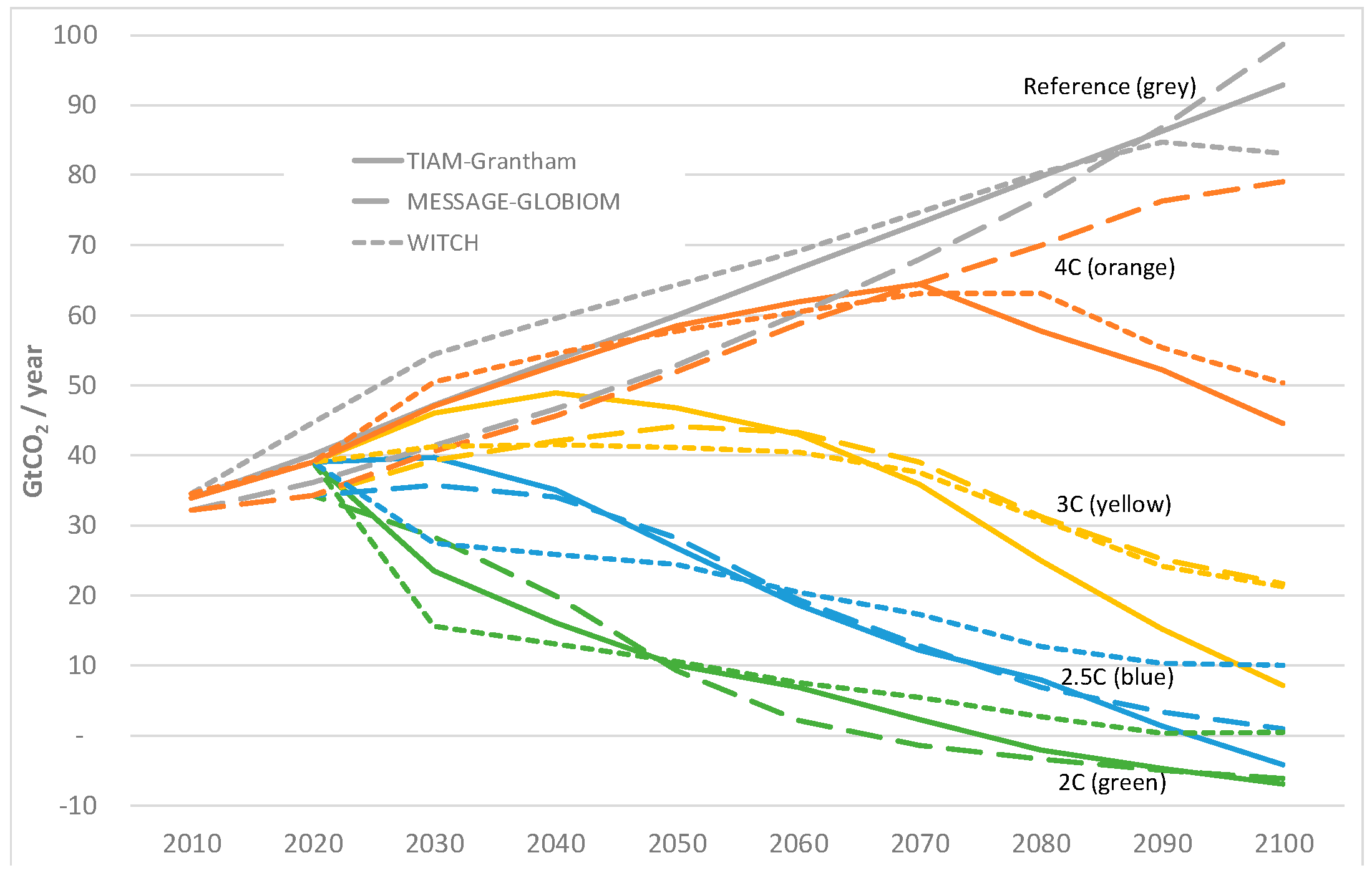
3.2. Can the Models Achieve the Different Temperature Goals?

If global coordinated mitigation action is delayed until 2030, two models (WITCH, MESSAGE-GLOBIOM) can still technically meet the 21st century CO2 budget. The TIAM-Grantham model can only solve by relying in the last decade of the century on a theoretical “backstop” technology which mitigates CO2 at a cost of $10,000/tCO2. Its results have been included here for illustrative purposes only, since the level of backstop technology is an arbitrary choice and does not indicate scenario impossibility in an absolute sense. In principle it would be possible to specify a lower-cost backstop technology if it were considered feasible to deploy measures such as air capture or other CO2 removal technologies at lower costs.
In addition to the model solution considerations, two models (WITCH and TIAM-Grantham) show very large CO2 price shocks, as shown in Figure 3. In the WITCH model, the CO2 price increases from zero to $1400/tCO2 between 2030 and 2040, whilst in the TIAM-Grantham model, the CO2 price increases by more than $1000/tCO2 per decade from 2060 onwards. Such decadal rises in CO2 prices (with $1000/tCO2 equivalent to an increase of $270/bbl in the price of crude oil) have been suggested to be a useful indication of scenario infeasibility, as they would represent substantial shocks to the global energy-economic system [33]. In the MESSAGE-GLOBIOM model, the CO2 price increases more gradually, but this is largely as a result of much lower CO2 emissions growth in the period 2010–2030.

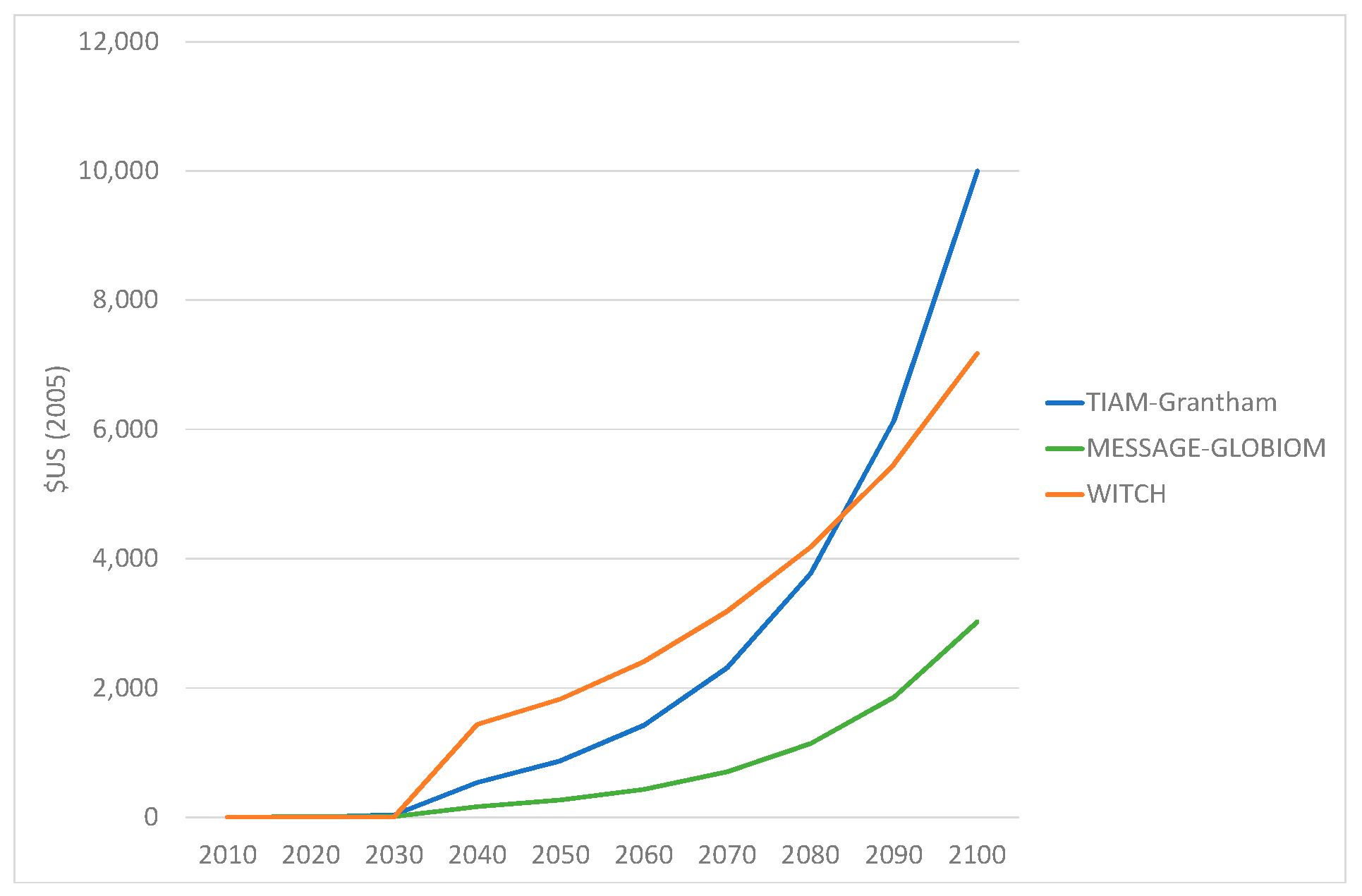
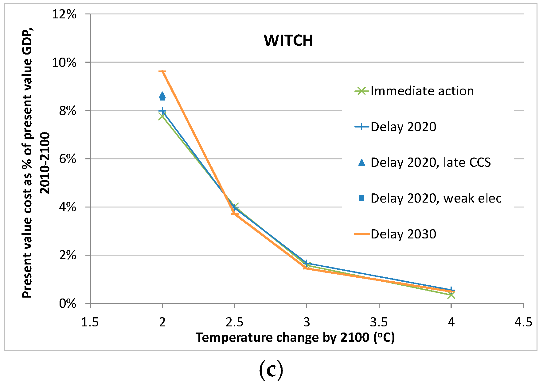
3.3. What is the Cost of Mitigation?

The measures of mitigation cost (as shown in Figure 4) reported by each of the three models is different. TIAM-Grantham reports the annual change in global welfare compared to the reference, as defined by the sum of changes in consumer and producer surplus, which is essentially the change in energy system cost once changes in energy service supply and demand (that result from changes in energy prices) have been accounted for. MESSAGE-GLOBIOM links the changes in energy prices from its energy-technology module to an aggregated macro-economic growth model, in order to investigate the changes in production and consumption of all goods and services (i.e., not just energy, as in TIAM-Grantham) that result from the mitigation scenario. WITCH reports a “policy cost”, which results from a more detailed macro-economic model, taking into account fully the general equilibrium effects of climate policies.
There is no simple relationship between how the mitigation cost is calculated and the magnitude of the cost, i.e., the degree to which a mitigation cost including a more complete set of macro-economic feedbacks leads to a larger or smaller cost compared to a cost based purely on the energy system technology costs [40]. However, mitigation costs calculated by only analysing energy system costs tend to be lower. In addition, technology availability and cost is a key determinant of mitigation costs across models. As can be seen from Figure 4, the relative mitigation costs between scenarios (indicated by the shape of the cost curves) are broadly similar across the three models, with an increasingly sharp rise in cost between the 3 °C and 2.5 °C, and the 2.5 °C and 2 °C scenarios, and with delayed global mitigation action and technology limitations leading to increased mitigation costs for the 2 °C scenarios in particular. The magnitude of mitigation costs is similar in TIAM-Grantham and MESSAGE-GLOBIOM, but in general much higher in WITCH.
The TIAM-Grantham and MESSAGE-GLOBIOM models’ mitigation costs for the 2°C scenario with immediate action and delayed action to 2020 (in a range of about 1.3%–1.7% of present value GDP to 2100) are similar to those found in previous AVOID studies which used variants of these models to assess regional mitigation costs for China and India [41,42,43]. The higher costs for the WITCH model reflect its macro-economic structure, which includes a production function with energy supply technologies “nested” together and with limited substitutability, which may be too rigid to reflect longer-term possibilities for low-carbon technologies to replace high-carbon technologies in the energy supply sectors. In addition, there are limited mitigation options in the transport sector within the model. Combined, these tend to result in much higher mitigation costs.
Across all three models, the global cost range for achieving the 2 °C scenarios spans 1.1%–10% of present value GDP to 2100 (equivalent to $34–288 trillion). This order of magnitude difference has been reported in previous modelling exercises, notably Clarke et al. [44] whose Energy Modelling Forum 22 (EMF 22) study showed present value mitigation costs for a 450 ppm scenario ranging from $12–120 trillion over the century.

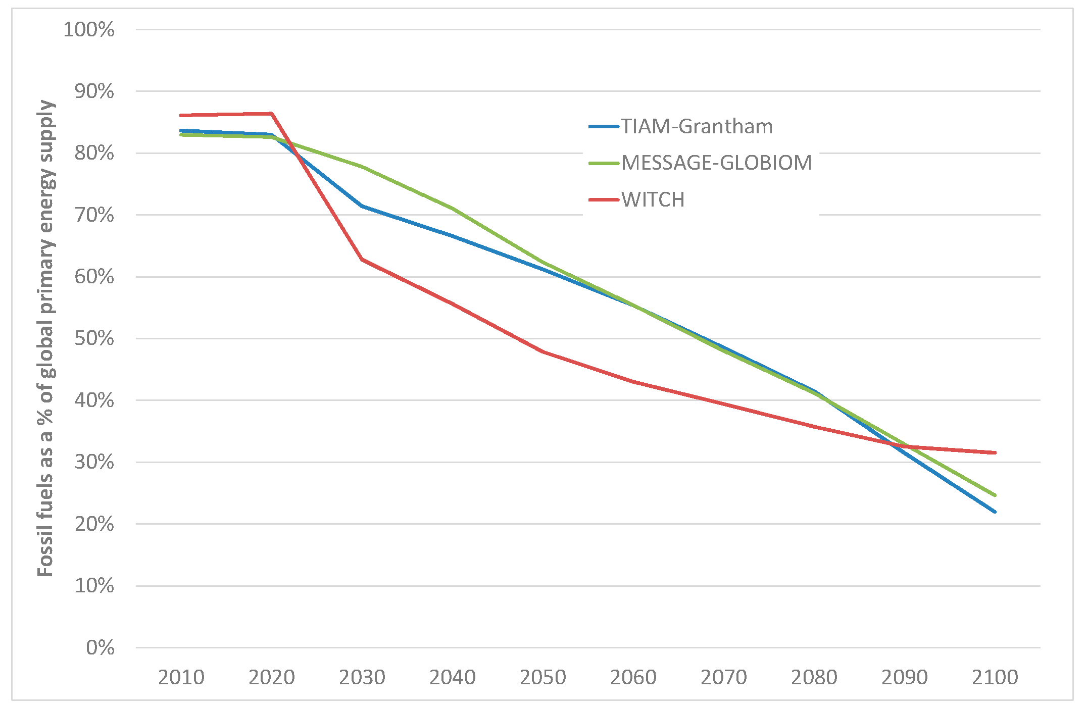
3.4. How Fast Does the Energy System Decarbonise?

Table 4 shows the average annual rate of global CO2 emissions reductions in the decade following the start of global mitigation action, for each temperature goal. Energy system decarbonisation rates are very rapid in the most delayed 2 °C scenario, in which global coordinated mitigation action towards the 2 °C goal doesn’t begin until 2030. The most drastic decarbonisation decade is that following the start of such mitigation action (2030–2040) which sees global CO2 emissions fall by an average 7%–14% per annum. Where action is delayed until 2020, the 2020–2030 decade sees average annual CO2 emissions reductions of 2%–8% per annum.
For the higher temperature goals, rates of decarbonisation are much less rapid. For the 2.5 °C scenarios, two models (TIAM-Grantham and MESSAGE-GLOBIOM) show emissions continuing to rise in the immediate action scenarios and in the case of MESSAGE-GLOBIOM in the delay to 2020 scenario as well. The highest decarbonisation rate is for the WITCH model (−5.7% per year) when action is delayed until 2030. For the 3 °C and 4 °C goals, in almost all modelled scenarios, CO2 emissions actually continue to grow in the decade following the start of global mitigation action.
As recently as 2010, decarbonisation rates in excess of 3% per annum were deemed to be “extreme”, based on a review of models at that time [13]. More recent analysis includes scenarios with delayed action beginning in 2030, in which average decarbonisation rates over the period 2030–2050 are also very high (5.9%–8.5%) [6]. This results from the models’ ability to rapidly substitute low-carbon for carbon-intensive technologies—a rapidity which can only be slowed by imposing explicit constraints on the models. Hence, the increasingly rapid rates of decarbonisation observed in the most recent assessments are a facet of the requirement to decarbonise at that rate in order to meet a given CO2, GHG or other emissions or climate target, given that emissions have continued to rise over time. Such rates have been compared to historic decarbonisation rates across countries, noting that countries such as France and Sweden achieved rates of 2%–3% per annum following the early 1970s oil crisis, but that at both a national and global scale, sustained rates as high as recently modelled are “unprecedented” [6]. A detailed analysis of the energy system changes across the century helps shed light on where the greatest challenges lie if such historic decarbonisation rates are to be exceeded.

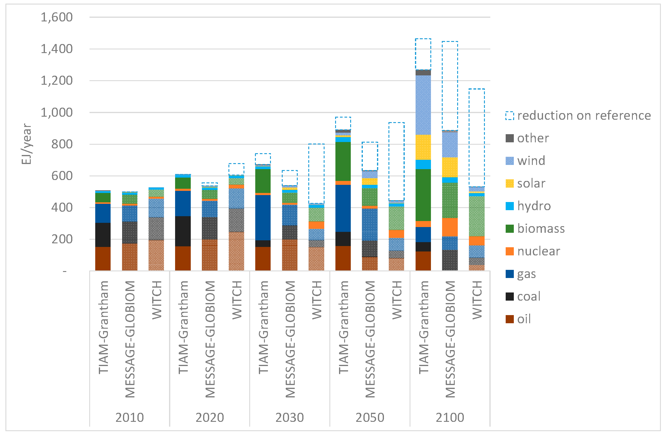
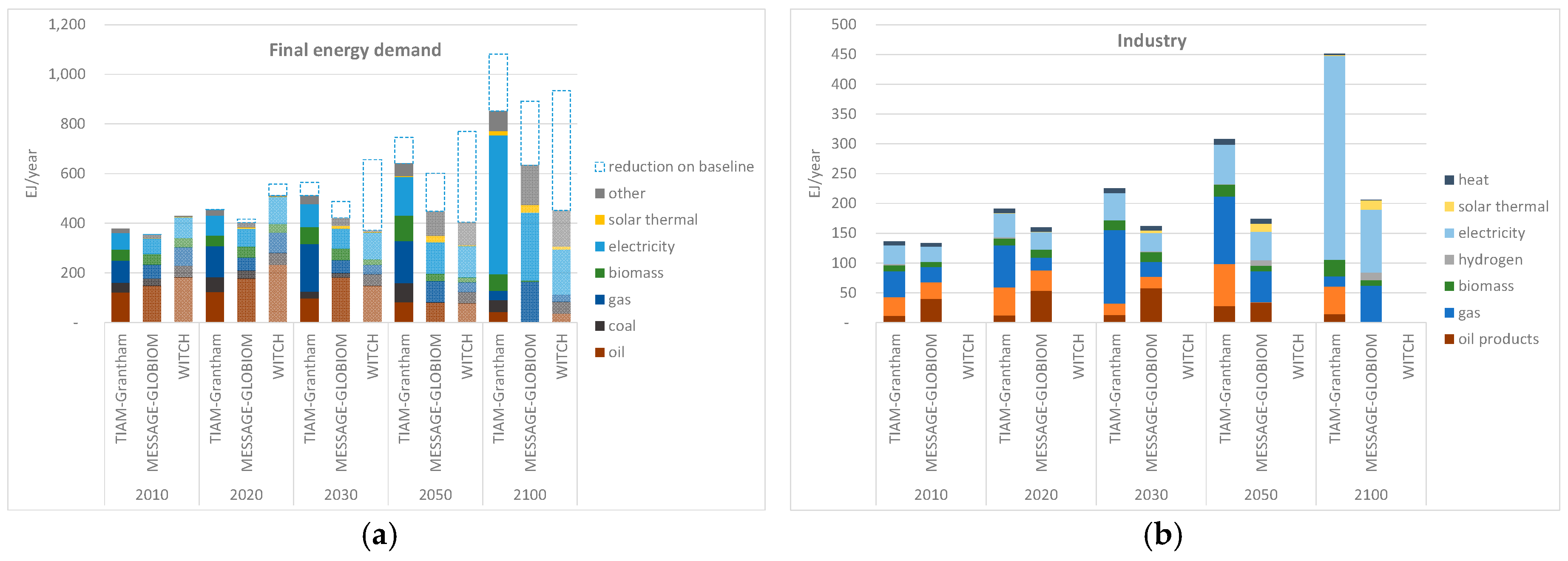
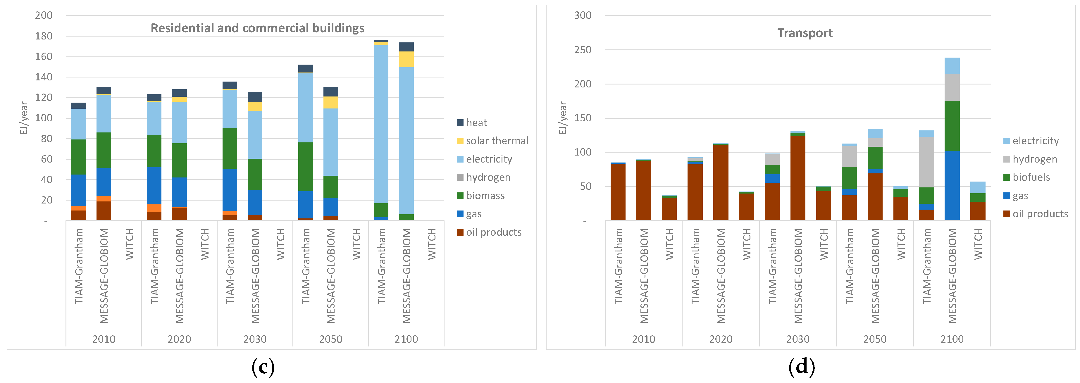
3.5. How Does the Energy System Change over the Century?

For the 2 °C scenario with mitigation action delayed until 2020, all models depend on a wide range of technologies and measures to meet the 2 °C goal, although to different extents for different technologies. Figure 5 shows that the fossil fuel share of primary energy reduces to 48%–62% by 2050 and to 22%–32% by 2100, compared to a level of more than 80% since 1970 [45]. Although total primary energy supply will increase by 2100, total fossil fuel supply will shrink.
As shown in Figure 6, the models show a broad range of primary energy supply reduction in the mitigation scenarios, with a 2100 value of 1150–1450 EJ/year in the reference reducing to 550–1250 EJ/year in the 2 °C scenario with delayed action to 2020. In the most extreme case, the WITCH model sees primary energy intensity of global GDP reduce from 7.8 MJ/$2005 in 2010 to 1.0 MJ/$2005 GDP by 2100—an average annual reduction of 2.3% per year. By contrast, TIAM-Grantham shows a reduction rate of 1.3% per year, and MESSAGE-GLOBIOM 1.7% per year. However, the annual average rates of reduction in the first decade following the start of global coordinated mitigation action are particularly high, ranging from 2.4% (TIAM-Grantham) to 6.8% (WITCH). These projected rates compare to historical primary energy reduction rates of 1.2% per year since 1970 [46]. Whilst these efficiency improvements are technically possible and reflected in other studies with a focus on maximising energy efficiency potential [46], it is unclear whether such a sector-wide, global improvement in energy efficiency is socially and politically realistic.
In the model with the highest energy intensity of GDP by 2100 (TIAM-Grantham), the 2 °C goal is achievedthrough a very significant shift of the energy system from fossil fuel-based to a mix of low-carbon sources dominated by wind, solar and biomass, as shown in Figure 6.
In each model, the electricity sector sees a fundamental shift from a system dominated by fossil fuel (mostly coal), nuclear and hydro in 2010 to a broad mix of renewables, nuclear and coal and gas with CCS by 2100, as shown in Figure 7. The increase in electricity generation in the TIAM-Grantham model is particularly striking, with a ten-fold increase in electricity generation between 2012 and 2100, reflecting that, in the latter half of the century, electricity increases as a share of final energy from 24% in 2050 (compared to about 18% today [47]) to 66% in 2100, dominated by buildings (88%) and industry (75%).
There is some variation between models in terms of the electricity generation technologies favoured. The period to 2050 sees a rapid penetration of CCS, which is already responsible for almost half of power generation globally by 2030 in the TIAM-Grantham model, and about 30% of generation in WITCH and MESSAGE-GLOBIOM. Nuclear takes a significant share of generation in WITCH and MESSAGE-GLOBIOM by 2100, whilst it is far less rapidly deployed in TIAM-Grantham, particularly compared to solar PV and CSP, as well as onshore wind. Although for all models nuclear is one of the more expensive technologies in capital cost terms (see Figure 8), its relatively large-scale deployment in WITCH and MESSAGE-GLOBIOM reflects the technology’s potential for supplying low-carbon, base-load power. In contrast, solar PV and wind are constrained in the models by the intermittency and variability of the resource.
Table 5 shows the deployment rates of key low-carbon technologies in the decade following the start of global mitigation action in the 2 °C scenarios with action starting in 2020 and 2030. The table is limited to show only those technologies requiring a build rate of greater than 30 GW per year on average (i.e., 300GW or more per decade). Rates of 30 GW per year have been achieved in key technologies including solar PV, nuclear and (on and offshore) wind, which is why deployment rates below this level are not deemed particularly challenging.
Table 5 indicates that a major challenge will include achieving hundreds of GW of installed CCS and nuclear capacity, with large-scale deployment starting as early as 2020 in the 2 °C scenario with action starting in 2020. Whilst these technology choices are not prescriptive, but rather indicate what would be deployed in a least-cost scenario without specific deployment constraints, they nevertheless highlight the potential importance of CCS and nuclear in achieving rapid decarbonisation of an energy system deeply reliant on fossil fuel combustion. Table 5 also shows the power generation technologies deployed in a 2 °C scenario with delayed action to 2020, where CCS is not available until 2050 as well as where electrification rates are capped. The former scenario indicates the increased importance of nuclear and the importance of gas and biomass generation (without CCS) as well as solar (PV and CSP). The latter scenario, in which electricity demand is lower than the other scenarios, still sees significant requirements for CCS (with gas and biomass), wind and nuclear power. Hence, as relatively unproven technologies, there is an immense benefit to successfully demonstrating both CCS and biomass (with and without CCS) power generation.
Such rapid deployment rates of specific technologies are common to studies of this kind, with recent model inter-comparisons focused specifically on this issue showing median deployment rates of wind of between 600–1500 GW per decade, solar 1700 GW per decade and nuclear just below 500 GW per decade during the period 2030–2050 in 2 °C-consistent (in this case 450 ppm) scenarios with delayed action to 2030 [10,35]. On the demand side, the energy mix across end-use sectors changes significantly over time, as shown in Figure 9. Although economic growth is harmonised across models, they can obtain different compositions of growth by sector (i.e., by industrial, commercial and agricultural services). This, as well as differing energy efficiency improvement rates, explains why MESSAGE-GLOBIOM and TIAM-Grantham have different energy demand growth rates in the industrial and transport sectors. WITCH does not have a sectoral split for final energy demand although does separate out the light duty vehicles sector, as represented in Figure 9d.
The figure shows that in all three models, total final energy demand shifts to electricity over the century, most markedly in the TIAM-Grantham model, in which electricity increases from 17% of total final energy in 2012 to 66% in 2100. This includes the virtual complete electrification of the buildings sector (about 90% of final energy by 2100, a proportion also reflected in the MESSAGE-GLOBIOM model) and industry sector (about 75% of final energy by 2100). In the transport sector, all models show a significant shift from oil over the course of the century, with TIAM-Grantham favouring hydrogen (fuel cell) vehicles and MESSAGE-GLOBIOM showing a more balanced split between gas, electricity, hydrogen and biofuels, by 2100.

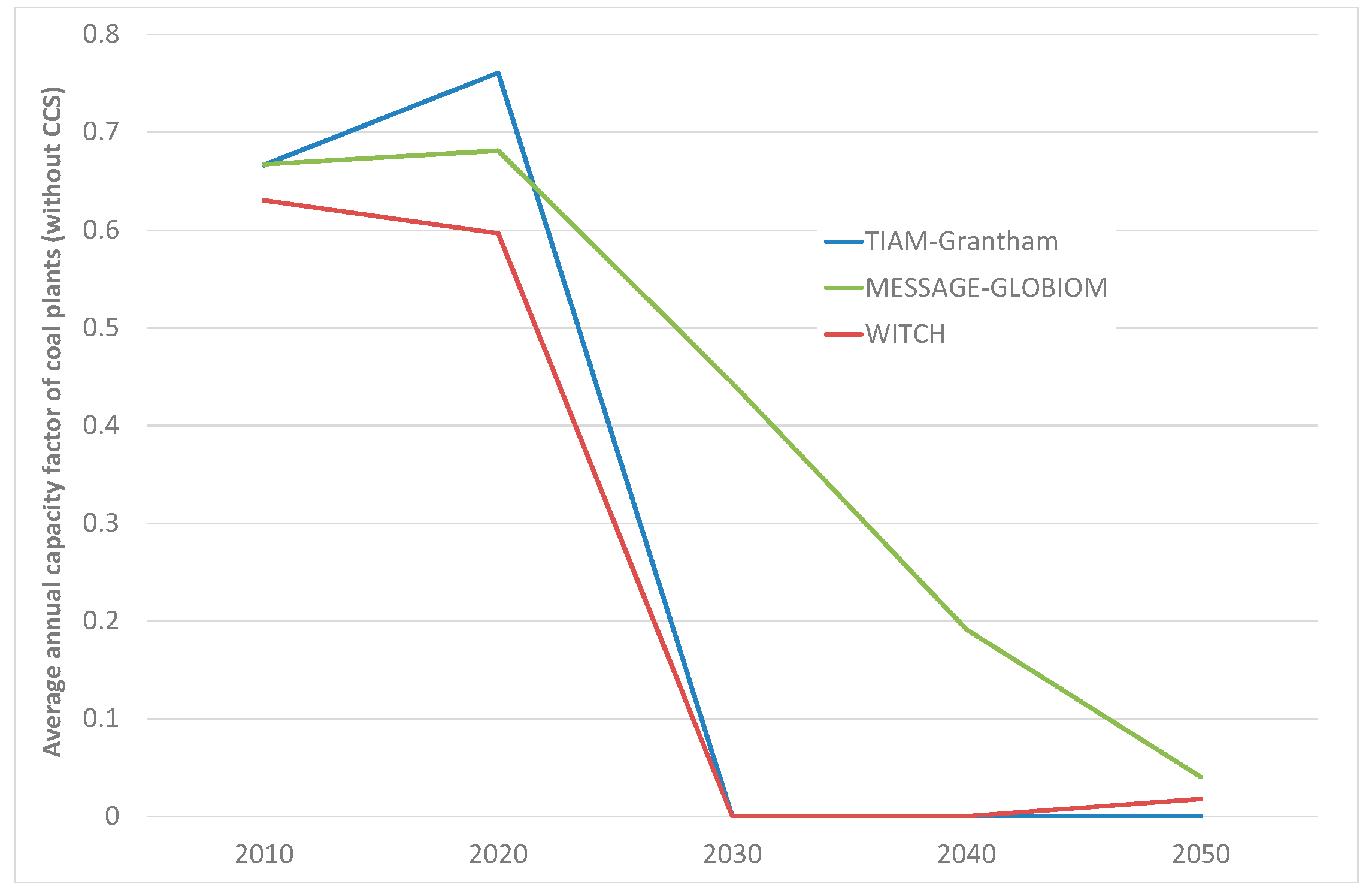
3.6. What Does Rapid Mitigation Imply for Coal-Fired Power Stations?

Even where global mitigation action begins in 2020, there are likely to be significant stranded coal plants as a result of rapid decarbonisation to meet the long term temperature goal of 2 °C, with average capacity factors falling to between 0 and 0.5 by 2030 (compared to 0.65 currently), as shown in Figure 10.
In two models (WITCH and TIAM-Grantham) the capacity factors fall to approximately zero, implying the early scrapping of 1400 GW of coal capacity by 2030. This is equivalent to scrapping 80% of existing economically viable coal capacity. Idling of coal plant has been explored in a previous study using a variant of the MESSAGE model with a broadly 2 °C-consistent goal, finding that an average of 350 GW of coal plant would be stranded on average over the period 2030–2050 if global mitigation action were delayed to 2030 [9]—a similar magnitude to the 450 GW of idled coal plant in MESSAGE-GLOBIOM in this study’s 2 °C scenario with delayed action until 2030.

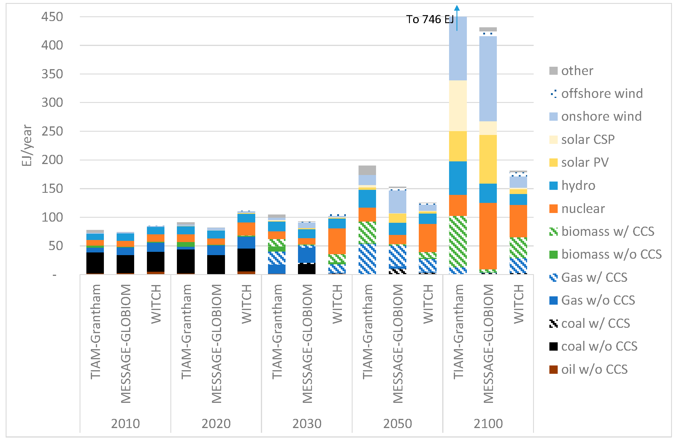
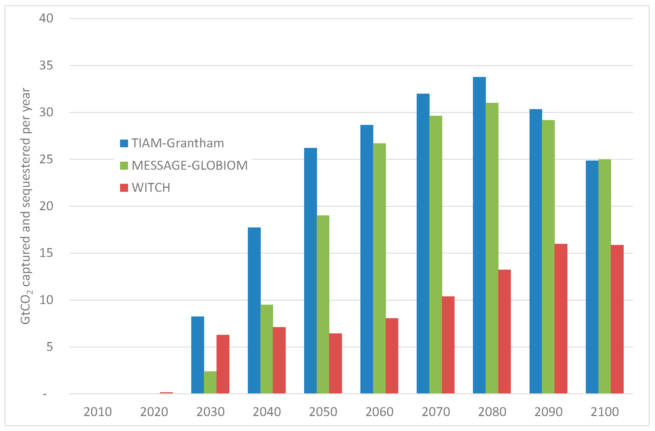
3.7. How Important is CO2 Capture in Achieving the Most Stringent Mitigation Scenarios?

To achieve the 2 °C goal, all models show a significant role for CO2 capture technologies, as illustrated in Figure 11. This peaks by 2080 in two models (TIAM-Grantham and MESSAGE-GLOBIOM) where 30–35 GtCO2/year (approximately the current CO2 emissions level) is being captured. In theory there is a sufficiently large global geological storage potential to accommodate this cumulative level of sequestration, which in the TIAM-Grantham model (which has the highest cumulative level of sequestration) reaches 1900 GtCO2 by 2100, compared to estimates of storage of at least 2000 GtCO2 globally, with potentially much more [50,51]. This does, however, highlight the importance of CCS, which must be sufficiently developed to be deployed at scale as soon as possible. With delayed CCS, mitigation costs increase very significantly, with half a percentage point of GDP lost over the century (as shown in Figure 4). This compares to an almost doubling of mitigation cost if there is no CCS at all [6].
Figure 12 highlights the degree to which global CO2 emissions become negative as a result of delays to global coordinated mitigation action. In the scenario with delayed action to 2020, one of the models (TIAM-Grantham) has net negative emissions by 2070, whilst MESSAGE-GLOBIOM has net negative emission by 2080. In the scenario with delayed action to 2030, all three models show net negative emissions by 2080, with TIAM-Grantham have more significant net negative emissions by 2070, and MESSAGE-GLOBIOM net negative emissions by 2070. As shown in Figure 12, across the three models, net negative emissions happen between 5 (TIAM-Grantham) and 25 (WITCH) years earlier with the 10-year delay in mitigation action.
To a large extent this reflects the RCP2.6 scenario originally presented in the literature, with net negative emissions by around 2070, even where mitigation action begins immediately [52]. This conclusion is also reflected in other assessments such as the UNEP Emissions Gap report, whose scenarios have net zero emissions achieved between 2060 and 2080 [23].
A significant driver of net negative emissions is bio-energy with CCS (BECCS) technology, in which net sequestration of atmospheric CO2 occurs, through the use of biomass to generate electricity or produce biofuels, with capture of CO2 in these processes. Figure 13 shows the growing importance of BECCS over the century in each model, in the 2 °C scenario with global mitigation action delayed until 2020. The economic and biophysical challenges of deploying large quantities of BECCS and other negative emissions technologies indicate that those scenarios which are highly reliant on BECCS are likely to face greater challenges [37,38].

3.8. A Matrix of Feasibility Indicators to Assess the Challenges of Different Mitigation Scenarios

The results presented and discussed in the previous sub-sections of Section 3 highlight a number of challenges to achieving the mitigation scenarios, in particular those with the most stringent temperature goal (i.e., 2 °C) and with the most delayed action or constrained technologies.
Table 6 sets out a (subjective) judgement on the degree of challenge associated with achieving each of the 2 °C scenarios explored in this model inter-comparison exercise. The 2 °C scenario with immediate action (in which action started from the models’ base years of 2010 or 2012) is excluded from this analysis, since it has been included purely as a hypothetical scenario, which is in fact no longer attainable. The table suggests that the 2 °C scenario with action delayed to 2030 is the most challenging when considering the full range of criteria. It is a clear indication for the need to commence global mitigation action towards a 2 °C-consistent CO2 budget as early as possible in the decade 2020–2030. This is all the more pertinent given that, as stated in Section 2, the delayed action until 2030 scenario is (at a global level of effort) broadly commensurate with the INDC pledges already made in the Paris Agreement process. The clear indication is that a ramping up of ambition in the 2020–2030 period is critical to increasing the feasibility of achieving a 2 °C target.
Table 7 shows the same multi-dimension comparison for the different temperature goals explored in this study, in each case for a scenario in which global coordinated mitigation action begins in 2020. This highlights that the degree of relative challenge of the 2 °C scenario across almost all dimensions of feasibility as measured in this study contrasts starkly with the higher LTTG scenarios. Even the 2.5 °C temperature goal has several challenging aspects, including non-trivial carbon prices and mitigation costs, potentially rapid near-term technology deployment rates across a range of low-carbon technologies, as well as potential idling of coal plants in the near-term and negative emissions in the long-term. By contrast, a global CO2 pathway which limits median warming in 2100 to 3 °C or above looks eminently achievable (which is encouraging given that scenarios with low or no mitigation action could lead to median 2100 temperature changes in excess of 4 °C [1]).
What about the Paris Agreement’s longer-term aims to achieve a “well below 2 °C” limit to global warming [52]? A sensitivity analysis using just the TIAM-Grantham model serves to highlight the additional difficulty of achieving long-term temperature change of less than 2 °C. Table 8 shows a direct comparison between the 2 °C scenario with global mitigation action beginning in 2020, and a further scenario in which a lower temperature change goal is achieved from the same 2020 starting point, in line with a cumulative fossil fuel combustion and industrial process CO2 emissions level of 1100 GtCO2 over the 21st century, compared to 1340 GtCO2 for the 2 °C scenario. This results in a median temperature change in 2100 of 1.85 °C, according to the analytical framework set out in Appendix D. It is therefore arguably not well below 2 °C and certainly some way off 1.5 °C, but it represents the lowest feasible scenario that can be attained in this set-up of the TIAM-Grantham model (i.e., with the socio-economic drivers and technology availability in the model that is used in the rest of this study).
As shown in Table 8, the implications of this more stringent mitigation scenario are even more challenging than those for the 2 °C scenario: earlier onset of rapid CO2 price increases; significantly higher mitigation costs; significantly higher initial rates of decarbonization, and marginally higher initial rates of energy intensity reduction; much higher initial deployment rates of low-carbon energy technologies; and earlier onset of significant carbon capture, with global net negative emissions a decade earlier than for the 2 °C scenario. As such, achieving even marginally more mitigation compared to the 2 °C scenario requires significant changes to the energy system in the TIAM-Grantham model. More recent analysis of the well below 2 °C reinforces that this challenge is likely to be felt across many dimensions including costs, stringency of near-term mitigation and reliance on negative emissions technologies [53,54,55]. In addition, these challenges are only quantified here and in these other studies across economic and technical dimensions, rather than across political and social dimensions. A key area of further research will be to better characterize these political and social dimensions so that we can judge more conclusively how likely it is that we can transform the energy system as quickly and fundamentally as necessary to achieve the Paris Agreement’s aims.

4. Discussion

Consideration of the different metrics associated with the modelled mitigation scenarios, as combined into the matrix presented in Section 3.8, highlights the following critical points affecting the feasibility of meeting the 2 °C goal:
  • Ensuring that mitigation action at a global level in line with the target begins as soon as possible, given the significant costs of delays, particularly to 2030, which implies the need for a ramping up of ambition over and above the currently submitted INDCs;
  • Achieving sustained energy efficiency improvements over the course of the century and very rapid near-term improvements, which though technically feasible, would be unlikely to occur without very effective policies;
  • Ensuring commercial-scale deployment of CCS is feasible as soon as technically and economically possible, such that hundreds of GW of CCS power stations can be deployed in the coming decades;
  • Developing supply chains for other low-carbon technologies such as wind, biomass, solar and nuclear to ensure that hundreds of GW globally can be deployed each decade in the near future;
  • Demonstrating the different aspects of BECCS technology and/or other negative emissions technologies so that global CO2 emissions can become first neutral and then net-negative in the latter half of the century;
  • Increasing the penetration of electricity-using heating, transport and industrial process technologies throughout the end-use sectors;
  • Managing the political economy issues that would be associated with the early idling of coal-fired power stations without CCS fitted.
A comparison of scenarios aimed at achieving a range of LTTGs (between a 2 °C and 4 °C median warming in 2100) also highlights that achieving the 2 °C goal (even if global coordinated mitigation action were to begin in 2020) is highly challenging compared to less stringent temperature goals. The analysis suggests that even a 2.5 °C temperature change may be relatively challenging, in terms of mitigation costs, required rates of deployment of key low-carbon technologies, and in some cases possible idling of coal plants in the near-term, plus negative emissions in the long-term.
Finally, a sensitivity analysis of the TIAM-Grantham model to going below 2 °C (specifically to 1.85 °C) suggests that almost all dimensions of feasibility explored here look significantly more challenging than even the 2 °C goal. This is of direct relevance to the current United Nations Framework Convention on Climate Change (UNFCCC) process which is seeking to raise ambition compared to Parties’ current Nationally Determined Contributions, in line with achieving a long-term temperature change of well below 2 °C and towards 1.5 °C [24].
In conclusion, the challenges associated with achieving a below 2 °C limit to temperature change are made clearer by highlighting the many relevant outputs of modelled scenarios against each-other, and suggest that the Paris Agreement targets will be extremely challenging. Application of this approach when modelling future low-carbon pathways aimed at achieving the most ambitious temperature limit of the Paris Agreement, at 1.5 °C, is recommended. Scenarios which outline what might be required to meet such stringent mitigation goals are of limited value without a clear and systematic assessment of the feasibility and degree of challenge involved in meeting those goals. This study makes a first attempt to systematize this feasibility assessment, whilst accepting that further research which more explicitly includes political and social dimensions should also be pursued to arrive at a more complete picture of how realistic our long-term climate change goals actually are.

Acknowledgments

This work was undertaken as part of the AVOID 2 research programme funded by the UK Government under Contract Reference Number 1104872. Further details of AVOID 2 are available at www.avoid.uk.net. Open access funds provided by Imperial College London.

Author Contributions

Ajay Gambhir and Jason Lowe conceived and designed the scenarios; Ajay Gambhir, Tamaryn Napp and Adam Hawkes ran the TIAM-Grantham model. Laurent Drouet and Valentina Bosetti ran the WITCH model. David McCollum, Oliver Fricko, Petr Havlik and Keywan Riahi ran the MESSAGE-GLOBIOM model. Dan Bernie and Jason Lowe ran the climate models. Tamaryn Napp, Ajay Gambhir, Laurent Drouet and David McCollum analysed the model outputs. Ajay Gambhir wrote the paper.

Conflicts of Interest

The authors declare no conflict of interest. The founding sponsors had no role in the design of the study; in the collection, analyses, or interpretation of data; in the writing of the manuscript, and in the decision to publish the results.

Appendix A. Regional CO2 Emissions in 2020 and 2030 for Moderate Action

Table A1 and Table A2 show the 2020 emissions pledges for Annex I and Non-Annex I countries under their “weak” (lower ambition) Cancun pledges. There are four categories of country to consider for the weak Cancun pledges scenario:
(1)
Countries which have offered unilaterally to meet an absolute CO2 or GHG emissions reduction on a specified base year. The EU, for example, has pledged that its 2020 GHG emissions are 20% below 1990 levels by 2020. The 2020 emissions cap given such pledges is determined simply by taking the specified emissions reduction from the specified base year. In the case of the EU, unfortunately neither TIAM, WITCH nor MESSAGE represent the region distinctly, with countries spread over a Western and Eastern European region. As such, an assumption has been made that those countries in Western Europe would have a target of 25% below their 1990 value, whilst those in Eastern Europe would have a target of 5% below their 1990 level. This differentiation is in line with the effort share principles upon which the non-traded (i.e., non EU ETS) sectoral emissions target in the EU is distributed between Member States. The specific % reductions chosen follow from Croatia (an Eastern European country) having a target to achieve a 5% reduction on its 1990 emissions levels. The combination of the 25% Western European countries target with the 5% Eastern European countries target yields an average reduction across all EU28 countries of just less than 20%, so this simplified burden split is deemed an acceptable approximation.
(2)
Countries which have offered unilaterally to meet an emissions intensity reduction on a specified base year. This category applies to China and India, which have offered a 40% and 20% reduction on their 2005 emissions intensity respectively. The 2020 absolute emissions level under this weaker pledge is calculated by multiplying the 2005 absolute emissions level by the projected GDP growth over the period 2005–2020 (using SSP2 GDP projections) and then subtracting the specified % reduction.
(3)
Countries which have made a pledge based on capping emissions at a specified %age below a 2020 Business as Usual (BAU) level. Countries such as Brazil and Indonesia have made such pledges. In the case of these countries an appropriate BAU estimate is required. This has been calculated by first taking the 2005 emissions level, and then by applying a BAU emissions growth factor over the period 2005 to 2020. The latter factor has been derived from den Elzen et al. [56], which covers all GHG emissions and land use change (whereas this study is focused on energy and industrial CO2 only). Strictly speaking, the use of this factor could account for the fact that the economic growth projected in this study, using SSP2 figures, is different to that projected using den Elzen et al. [56]. However, many factors affect emissions growth, not just GDP, and so a simplifying assumption has been made to use the same factor.
(4)
Countries which have not made a pledge. This category applies to countries such as the USA, whose Cancun pledge is contingent on international action, and the majority of non-Annex I countries, who have stated qualitatively a series of nationally appropriate mitigation actions (NAMAs). In many cases, it makes most sense to simply not impose a cap on regions representing these countries—or combinations of these countries—in the TIAM, WITCH and MESSAGE models. However, in some cases regions represented by the models include a combination of countries form this category, and countries from other categories. In these cases a projection of BAU emissions for these countries is required, before emissions for the different countries within the region can be aggregated up to a regional estimate of 2020 emissions. As for category 3, this category of countries therefore requires an assumption of BAU emissions in 2020, and the 2005–2020 emissions growth factor derived from den Elzen et al. [56] has again been applied to 2005 emissions.
Table A1. Details of Cancun pledges (where quantified)—Annex I [57].
Country/RegionWeak PledgeStrong Pledge
AustraliaGHG 5% below 2000 by 2020GHG 25% below 2000 by 2020
BelarusEmissions 5% below 1990 by 2020Emissions 10% below 1990 by 2020
CanadaNoneGHG 17% below 2005 by 2020
CroatiaEmissions 5% below 1990 by 2020Emissions 5% below 1990 by 2020
EUGHG 20% below 1990 by 2020GHG 30% below 1990 by 2020
IcelandGHG 15% below 1990 by 2020GHG 30% below 1990 by 2020
JapanNoneGHG 25% below 1990 by 2020
Kazakhstan15% below 1992GHG 25% below 1990 by 2020
New ZealandGHG 10% below 1990 by 2020GHG 20% below 1990 by 2020
NorwayGHG 30% below 1990 by 2020GHG 40% below 1990 by 2020
Russian FederationGHG 15% below 1990 by 2020GHG 25% below 1990 by 2020
SwitzerlandGHG 20% below 1990 by 2020GHG 30% below 1990 by 2020
UkraineGHG 15% below 1990 by 2020GHG 20% below 1990 by 2020
USANoneGHG 17% below 2005 by 2020
Table A2. Details of Cancun pledges (where quantified in % reduction terms)—Non-Annex I. BAU: business as usual [58].
Country/RegionWeak PledgeStrong Pledge
BrazilGHG 36.1% below 2020 BAU by 2020GHG 38.9% below 2020 BAU by 2020
ChileGHG 20% below 2020 BAU by 2020GHG 20% below 2020 BAU by 2020
ChinaGHG intensity 40% below 2005 in 2020GHG intensity 45% below 2005 in 2020
IndiaCO2 intensity 20% below 2005 levels in 2020CO2 intensity 25% below 2005 levels in 2005
IndonesiaNoneGHG 26% below 2020 BAU by 2020
IsraelGHG 20% below 2020 BAU by 2020GHG 20% below 2020 BAU by 2020
MexicoNoneGHG 30% below 2020 BAU by 2020
Papua New GuineaNoneGHG 50% lower by 2030
South KoreaGHG 30% below 2020 BAU by 2020GHG 30% below 2020 BAU by 2020
Rep of MoldovaGHG 25% below 1990 by 2020GHG 25% below 1990 by 2020
SingaporeNoneGHG 16% below 2020 BAU by 2020
South AfricaNoneGHG 34% below 2020 BAU by 2020
For categories 3 and 4, in many cases the pledges result in emissions higher than the BAU projected in den Elzen et al. [56]. In such cases the pledge has been assumed to be the BAU in 2020.
Because of its relative granularity in terms of regions described, the IEA’s World Energy Outlook (WEO) 2013 [59] data has formed the basis of finding a ratio of 2030 emissions/2020 emissions in a weak policy scenario (what the WEO 2013 calls the “New Policies Scenario”. WEO regions which are broadly the same as those in the TIAM model have been used to derive the uplift (or downward shift) in emissions from 2020 to 2030. This results in the global emissions levels shown in Table A3, with comparisons to the European Commission-funded “Ampere” study [6] also shown.
Table A3. Global CO2 emissions in this study compared to others, for 2020 and 2030.
Study2020 Global Emissions from Fossil Fuels and Industry2030 Global Emissions from Fossil and IndustryComment
This study38,98141,4222030 emissions 6% higher than 2020
WEO 201334,595 (excluding industry)36,4932030 emissions 5% higher than 2020 (Excludes cement)
Ampere WITCH39,73146,4062030 emissions 17% higher than 2020
Ampere MESSAGE38,18242,3442030 emissions 11% higher than 2020
The assumptions, based on IEA WEO 2013, show a relative flattening of global emissions between 2020 and 2030, when compared to the WITCH and (to a lesser extent) MESSAGE Ampere studies. However, the SSP2 growth rates at a global level are reasonably close to those used in WEO 2013, and there are few other regionally disaggregated sources of information on 2030 emissions pledges under a weak policy scenario. Finally, the differences between these assumed rates of emissions growth between 2020 and 2030 are likely to be relatively trivial when compared to the significant deviation from the weak policy pathway in order to achieve the 2 °C pathway.

Appendix B. Capped Electrification Rates for Different Regions in Each Model

In order to simulate a scenario in which limited progress is made in developing electric end-use technologies in the transport, buildings and industrial sectors, caps have been placed on the share of total final energy demand in each end-use sector in each region. Table B1 shows the caps applied in each case. These were derived with reference to recent (2011) shares of final energy demand made up by electricity for each region and sector, as well as those shares in 2035 in scenarios where only current policies are implemented, as gleaned from the IEA’s WEO 2013 [59].
Table B1. Cap on % share of electricity in final energy use for each major end-use sector. Notes: Sectoral abbreviations as follows: IND = Industry; TRA = Transport; BUI = Buildings. Regional abbreviations as follows: AFR = Africa; SSA = Sub Saharan Africa; AUS = Australia, New Zealand and Oceania; PAC = OECD Pacific; KOS = South Korea, South Africa and Australia; CAN = Canada; CAJ = Canada, Japan and New Zealand; CHI = China; CPA = Central and Planned Asia; CSA = Central and South America; LAC = Latin America and Caribbean; LAM = Latin America, Mexico and Caribbean; EEU = Eastern Europe; CEE = Central and Eastern Europe; FSU = Former Soviet Union; TE = Non-EU Eastern European countries including Russia; IN = India; SAS = South Asia; JAP = Japan; ME = Middle East; MEA = Middle East and North Africa; MEX = Mexico; ODA = Other Developing Asia; OPA = Other Asia Pacific; SEA = South East Asia; USA = USA; NAM = North America; WEU = Western Europe.
TIAM-GranthamMESSAGE-GLOBIOMWITCH
RegionINDTRABUIRegionINDTRABUIRegionINDTRABUI
AFR30520AFR30520SSA30520
AUS40560PAC40560KOS40560
CAN40560----CAJ40560
CHI40550CPA40550CHI40550
CSA30560LAC30560LAM30560
EEU301030CEE301030EEU301030
FSU301030FSU301030TE301030
IN30540SAS30540SAS30540
JAP40555--------
ME20560MEA20560MEA20560
MEX40540--------
ODA40540OPA40540SEA40540
SKO40540--------
USA40560NAM40560USA40560
WEU40540WEU40540WEU40540
For the buildings and industry sectors, in all cases the current share of electricity in each end-use sector in each region has been rounded up to the nearest 10%. For transport, in almost all regions a cap of 5% has been opposed, reflecting the fact that the current and (in current policies scenarios) future share of electricity in transport remains very small (at 1% or 2%). The exception is in the Former Soviet Union and Eastern European countries, where the electricity share of transport final energy demand is between 5% and 10%.

Appendix C. Model Descriptions

IIASA operates the MESSAGE-GLOBIOM integrated assessment modelling framework. MESSAGE is an energy engineering model based on a linear programming (LP) optimization approach which is used for medium- to long-term energy system planning and policy analysis [14,27,28]. The model minimizes total discounted energy system costs, and provides information on the utilization of domestic resources, energy imports and exports and trade-related monetary flows, investment requirements, the types of production or conversion technologies selected (technology substitution), pollutant emissions, and inter-fuel substitution processes, as well as temporal trajectories for primary, secondary, final, and useful energy. MESSAGE is coupled to GLOBIOM [60] to analyse the competition for land use between agriculture, forestry, and bioenergy, which are the main land-based production sectors. It accounts for the 18 most globally important crops, a range of livestock production activities, forestry commodities, first- and second-generation bioenergy, and water. The comprehensive coverage of all energy and land sectors allows assessing emissions and mitigation options for the full basket of greenhouse gases and other radiatively active substances [61]. To estimate regionally-aggregated, sector-based air pollutant emissions and related pollution control costs, MESSAGE has been linked to the GAINS model [62,63]. For the estimation of price-induced changes of the energy demand, MESSAGE-GLOBIOM is iterated with the macro-economic model MACRO [64]. In MACRO, capital stock, available labour, and energy inputs determine the total output of the economy according to a nested constant elasticity of substitution (CES) production function. Through the linkage to MESSAGE-GLOBIOM, internally consistent projections of GDP and energy demand are calculated in an iterative fashion that takes price-induced changes of demand and GDP into account. Furthermore, MESSAGE-GLOBIOM is used in conjunction with MAGICC (Model for Greenhouse gas Induced Climate Change) version 6 [65] for calculating internally consistent scenarios for climatic indicators such as atmospheric concentrations, radiative forcing, annual-mean global surface air temperature and global-mean sea level implications.
TIAM-Grantham is the Grantham Institute, Imperial College London’s version of the ETSAP-TIAM model, which is the global, 15-region incarnation of the TIMES model generator [25,26], as developed and maintained by the Energy Technology Systems Analysis Programme (ETSAP). The model is a LP tool representing in rich resource and technological detail all elements of the reference energy system (RES) for each region represented, mapping energy commodity flows all the way from their extraction and refining to their distribution and end-use. TIAM has the ability to optimise the energy system for given climate constraints through either minimising the total discounted energy system cost over a given time-horizon, or through minimising total producer and consumer welfare when (optionally) accounting for elastic demand responses to energy prices. In the latter case, the model is solved as a partial equilibrium. There is no linkage to a macroeconomic model to observe full equilibrium impacts of changes in energy prices. The model uses exogenous inputs of factors such as GDP, population, household size and sectoral output shares to project future energy service demands across the agricultural, commercial, industrial, residential and transport sectors in each region. Energy system data such as technology costs, resource supply curves and annual resource availability are also input into the model. In solving, the model allows trade in energy commodities between regions.
WITCH is a dynamic global model that integrates the most important elements of climate change in a unified framework [30]. The economy is modelled through an inter-temporal optimal growth model which captures the long-term economic growth dynamics. A compact representation of the energy sector is fully integrated (hard linked) with the rest of the economy so that energy investments and resources are chosen optimally, together with the other macroeconomic variables. WITCH represents the world in a number (in this study, 12) of representative native regions (or coalitions of regions); for each it generates optimal mitigation and adaptation strategies for the long term (2005 to 2100), as a result of a maximization process in which the welfare of each region (or coalition of regions) is chosen strategically and simultaneously to other regions. This makes it possible to capture regional free-riding behaviours and strategic interaction induced by the presence of global externalities. In this game-theory set-up, regional strategic actions interrelate through GHG emissions, dependence on exhaustible natural resources, trade of oil and carbon permits, and technology research and development. The endogenous representation of research-and-development diffusion and innovation processes constitutes a distinguishing feature of WITCH. This approach gives the possibility to explore how research-and-development investments in energy efficiency and carbon-free technologies integrate the currently available mitigation options. The model features multiple externalities, both on the climate and the innovation side. The technology externality is modelled via international spillovers of knowledge and experience across countries and time. This formulation of technical change affects both decarbonization as well as energy savings.

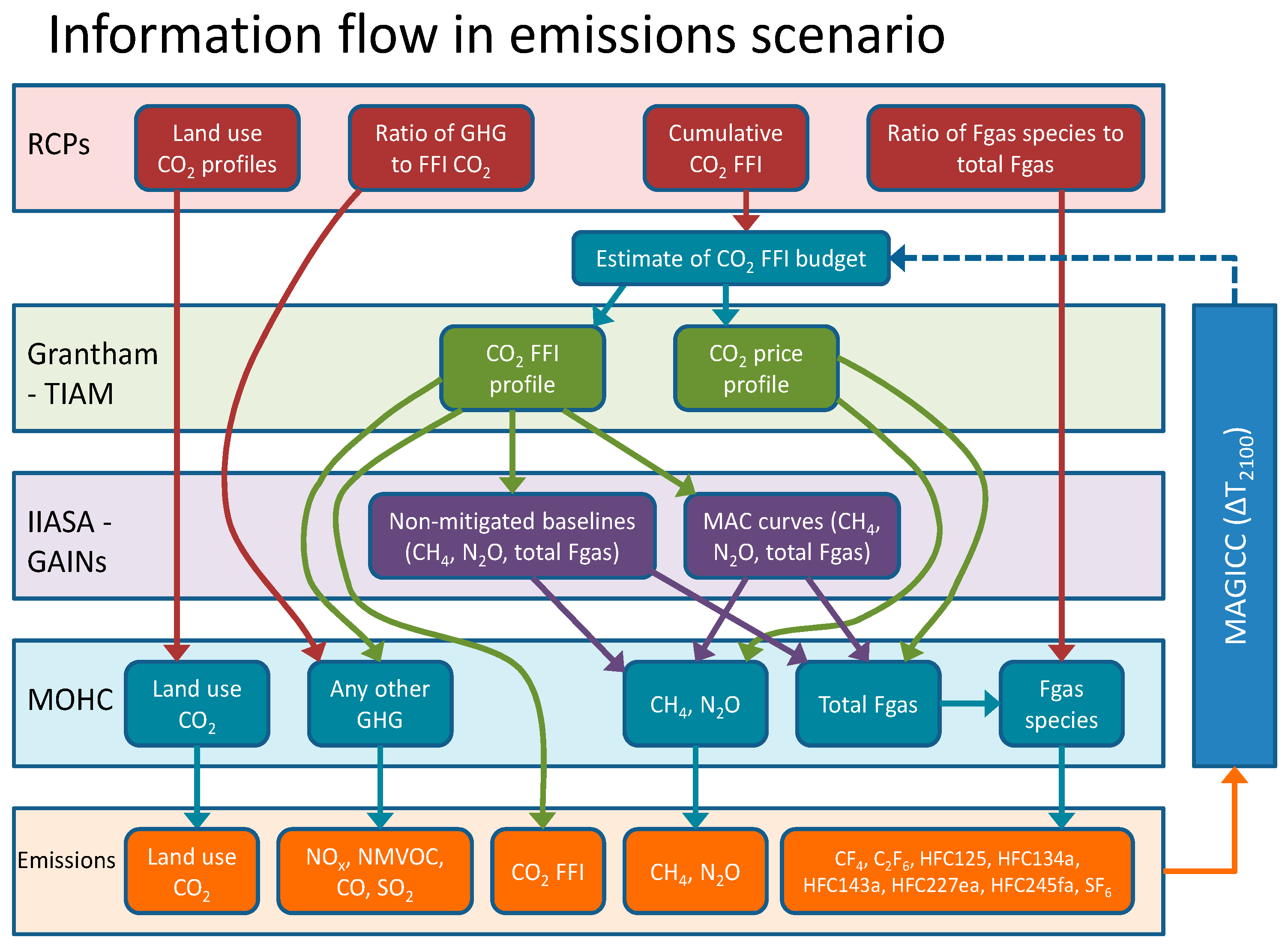
Appendix D. Deriving Temperature Goal-Consistent 21st Century CO2 Budgets and Emissions Profiles

The TIAM-Grantham and IIASA GAINS [66,67] models are used to derive time profiles of emissions of CO2, CH4, N2O and total F-Gas emissions from a given cumulative CO2 budget for fossil fuels and industry (FFI) in order to meet a given LTTG—the temperature change in 2100. In order to make climate projections (verifying the CO2 budgets) the total F-Gas emissions must be broken down into constituent species and emissions of other gases must also be estimated. The process of constructing the full set of emissions required and the iterative process used to determine the 21st century (i.e., 2000–2100) CO2 FFI budget is detailed here. A schematic of the information flow through the RCPs, TIAM-Grantham, GAINS and Met Office Hadley Centre (MOHC) calculations is illustrated in Figure 1.
(1)
Projections of global temperature change for the four RCPs is made using emissions relating to the RCPs [68]. Emissions are used rather than concentrations as this takes fuller account of uncertainty carbon cycle feedbacks. Following Bernie and Lowe [69], probabilistic projections are made using values of equilibrium climate sensitivity from models in the fifth Couple Model Inter-comparison Project (CMIP5) [70] along with uncertainty distributions of ocean mixing and carbon cycle feedbacks.
(2)
In each year land use emissions of CO2 are linearly interpolated from the RCPs on the basis of each RCP’s median 2100 projected temperature and the LTTG of the scenario.
(3)
Initial estimates of 21st century cumulative CO2 emissions from the FFI sectors are also linearly interpolated from the RCPs on the basis of future temperature projections and the scenario LTTG.
(4)
The cumulative CO2 FFI budget is then used to calculate emissions of CO2 from FFI, CH4, N2O and F-gases:
(a)
A time profile of CO2 emissions from FFI is then calculated from the cumulative CO2 FFI along with a carbon price profile;
(b)
The CO2 FFI emissions profile and aspects of the underlying energy system structure (in particular the fossil fuel energy mix) are then passed to GAINS to calculate non-CO2 GHG no-mitigation scenarios and corresponding marginal abatement cost (MAC) curves;
(c)
The CO2 FFI profile from TIAM-Grantham and the non-CO2 GHG no-mitigation scenarios and MAC curves from GAINS are then used to calculate the emissions of CH4, N2O and total F-Gas emissions, at different levels of CO2e price applied to the non-CO2 GHGs (using GWP100 values).
(5)
Individual F-gas emissions are then needed, but the constituent F-gases in the categories used by GAINS do not exactly match those used by MAGICC. Whilst this has a very small influence on the overall CO2e emissions, the individual gas species are needed by MAGICC. To estimate emissions of individual F-gases it is assumed that the relative emissions rate of each F-gas to the total F-gas emissions will change with time in line with the “unmitigated” RCP 8.5 scenario. Based on this assumption the emissions of each F-gas in RCP8.5 are scaled by a ratio of the total F-gas emissions from GAINS to the total F-gas emissions in the unmitigated reference scenario. So for example if the F-gas emissions from GAINS are 20% of the unmitigated F-gas emissions for that scenario, then this factor is applied to emissions of each individual F-gas from RCP8.5. This approach circumvents the issue of different gases being included in the calculation by GAINS and those needed by MAGICC. While other assumptions are possible, given the relatively small effect of differences in F-gas emissions between the RCPs, this an appropriate level of detail for the scope of the current study.
(6)
The emissions of non-Kyoto GHG and other gases needed by MAGICC (principally NOx, CO, NMVOC, SO2) are all based on the ratio of the emissions of each gas to the emissions of CO2 from the FFI sector in the RCPs being applied to the CO2 FFI emissions from TIAM-Grantham. For example if the CO2 FFI emissions from GAINS in a given year where 80% of the way between RCP4.5 and RCP6.0, the SO2 emissions would be the product of the CO2 FFI from TIAM-Grantham multiplied by a weighted mean of the ratio of SO2 to CO2 FFI in those two RCPs, with 4 times more weight given to the ratio from RCP6.0.
(7)
Projected median 2100 temperature change is then calculated and if within 0.1 °C of the original LTTG, the CO2 FFI budget is accepted, or else the CO2 budget for the scenario is re-estimated, before repeating the above procedure to re-calculate 2100 median temperature change.
It should be noted again that the temperatures resulting from the emissions derived from a given budget are verified as meeting the target. With the cumulative CO2 FFI being the only variable here the process used in iterating its value for each target warming level is unimportant. However, the use of a simple interpolation of cumulative CO2 emissions to determine eventual warming is a notion that has become widely accepted in recent years [71,72,73]. Its use here to initially estimate the CO2 budget for specific target warming levels implicitly assumes that the contribution of non-CO2 gases to warming is linearly related to the emissions of CO2. While this may appear to be broadly the case across the wide range of scenarios from the IPCC’s AR5 WGII report [1], the wide spread in IAM construction and the experimental design across the scenarios available is likely to obscure more subtle relations from IAM scenarios constructed under specific sets of assumptions on constraints. For example two scenarios with similar CO2 emissions profiles but which focus on either energy demand reduction or the heavy use of bio-energy with carbon capture and storage (BECCS) would likely have different non-CO2 contributions to warming. Similarly, emissions scenarios with different climate targets derived from a common approach, such as here, would not necessarily produce a robustly linear relation of warming to CO2 when the nuances of the underlying technological, economic and social assumptions and constraints are considered.
While the breakdown of the relation of cumulative emissions to temperature demonstrated by the need for iteration in developing these scenarios in small, it illustrates the inherent uncertainty in this relation and warrants careful verification of projections developed on this basis.

References

  1. Intergovernmental Panel on Climate Change (IPCC). Climate Change 2014: Mitigation of Climate Change. Contribution of Working Group III to the Fifth Assessment Report of the Intergovernmental Panel on Climate Change; Edenhofer, O., Pichs-Madruga, R., Sokona, Y., Minx, J.C., Farahani, E., Kadner, S., Seyboth, K., Adler, A., Baum, I., Brunner, S., et al., Eds.; Cambridge University Press: Cambridge, UK; New York, NY, USA, 2014. [Google Scholar]
  2. Dessens, O.; Anandarajah, G.; Gambhir, A. Limiting global warming to 2 °C: What do the latest mitigation studies tell us about costs, technologies and other impacts? Energy Strategy Rev. 2016, 13–14, 67–76. [Google Scholar] [CrossRef]
  3. O’Neill, B.C.; Kriegler, E.; Riahi, K.; Ebi, K.L.; Hallegatte, S.; Carter, T.R.; Mathur, R.; van Vuuren, D.P. A new scenario framework for climate change research: The concept of shared socioeconomic pathways. Clim. Chang. 2014, 122, 387–400. [Google Scholar] [CrossRef]
  4. Bernie, D.; Lowe, J.A. Future Temperature Responses Based on IPCC and Other Existing Emissions Scenarios. Available online: http://avoid-net-uk.cc.ic.ac.uk/wp-content/uploads/delightful-downloads/2015/02/AVOID2_WPA-1_final_v2.pdf (accessed on 30 November 2015).
  5. Clarke, L.; Jiang, K.; Akimoto, K.; Babiker, M.; Blanford, G.; Fisher-Vanden, K.; Hourcade, J.C.; Krey, V.; Kriegler, E.; Löschel, A.; et al. Assessing transformation pathways. In Climate Change 2014: Mitigation of Climate Change. Contribution of Working Group III to the Fifth Assessment Report of the Intergovernmental Panel on Climate Change; Edenhofer, O., Pichs-Madruga, R., Sokona, Y., Minx, J.C., Farahani, E., Kadner, S., Seyboth, K., Adler, A., Baum, I., Brunner, S., et al., Eds.; Cambridge University Press: Cambridge, UK; New York, NY, USA, 2014. [Google Scholar]
  6. Riahi, K.; Kriegler, E.; Johnson, N.; Bertram, C.; den Elzen, M.G.J.; Eom, J.; Schaeffer, M.; Edmonds, J.; Isaac, M.; Krey, V.; et al. Locked into Copenhagen pledges–Implications of short-term emission targets for the cost and feasibility of long-term climate goals. Technol. Forecast. Soc. Chang. 2015, 90, 8–23. [Google Scholar] [CrossRef] [Green Version]
  7. Kriegler, E.; Weyant, J.P.; Blanford, G.J.; Krey, V.; Clarke, L.; Edmonds, J.; Fawcett, A.; Luderer, G.; Riahi, K.; Richels, R.; et al. The role of technology for achieving climate policy objectives: Overview of the EMF 27 study on global technology and climate policy strategies. Clim. Chang. 2014, 123, 353–367. [Google Scholar] [CrossRef] [Green Version]
  8. World Energy Investment Outlook 2014; International Energy Agency (IEA): Paris, France, 2014.
  9. Johnson, N.; Krey, V.; McCollum, D.L.; Rao, S.; Riahi, K.; Rogelj, J. Stranded on a low-carbon planet: Implications of climate policy for the phase-out of coal-based power plants. Technol. Forecast. Soc. Chang. 2015, 90, 89–102. [Google Scholar] [CrossRef]
  10. Van der Zwaan, B.C.C.; Rösler, H.; Kober, T.; Aboumahboub, T.; Calvin, K.V.; Gernaat, D.E.H.J.; Marangoni, G.; McCollum, D. A cross-model comparison of global long-term technology diffusion under a 2 °C climate change control target. Clim. Chang. Econ. 2013, 4, 1340013. [Google Scholar] [CrossRef]
  11. Krey, V.; Luderer, G.; Clarke, L.; Kriegler, E. Getting from here to there—Energy technology transformation pathways in the EMF27 scenarios. Clim. Chang. 2013, 123, 369–382. [Google Scholar] [CrossRef]
  12. Rose, S.K.; Kriegler, E.; Bibas, R.; Calvin, K.; Popp, A.; van Vuuren, D.P.; Weyant, J. Bioenergy in energy transformation and climate management. Clim. Chang. 2013, 123, 477–493. [Google Scholar] [CrossRef]
  13. Den Elzen, M.G.J.; van Vuuren, D.P.; van Vliet, J. Postponing emission reductions from 2020 to 2030 increases climate risks and long-term costs. Clim. Chang. 2010, 99, 313–320. [Google Scholar] [CrossRef]
  14. Riahi, K.; Dentener, F.; Gielen, D.; Grubler, A.; Jewell, J.; Klimont, Z.; Krey, V.; McCollum, D.; Pachauri, S.; Rao, S.; et al. Energy pathways for sustainable development. In Global Energy Assessment—Toward a Sustainable Future; Cambridge University Press: Cambridge, UK; New York, NY, USA; International Institute for Applied Systems Analysis (IIASA): Laxenburg, Austria, 2012; pp. 1203–1306. [Google Scholar]
  15. Luderer, G.; Bertram, C.; Calvin, K.; Cian, E.D.; Kriegler, E. Implications of weak near-term climate policies on long-term mitigation pathways. Clim. Chang. 2013, 136, 127–140. [Google Scholar] [CrossRef]
  16. Luderer, G.; Pietzcker, R.C.; Bertram, C.; Kriegler, E.; Meinshausen, M.; Edenhofer, O. Economic mitigation challenges: How further delay closes the door for achieving climate targets. Environ. Res. Lett. 2013, 8, 34033. [Google Scholar] [CrossRef]
  17. Von Stechow, C.; Minx, J.C.; Riahi, K.; Jewell, J.; McCollum, D.L.; Callaghan, M.W.; Bertram, C.; Luderer, G.; Baiocchi, G. 2 °C and SDGs: United they stand, divided they fall? Environ. Res. Lett. 2016, 11, 34022. [Google Scholar] [CrossRef]
  18. Van Sluisveld, M.A.E.; Harmsen, J.H.M.; Bauer, N.; McCollum, D.L.; Riahi, K.; Tavoni, M.; van Vuuren, D.P.; Wilson, C.; van der Zwaan, B. Comparing future patterns of energy system change in 2 °C scenarios with historically observed rates of change. Glob. Environ. Chang. 2015, 35, 436–449. [Google Scholar] [CrossRef] [Green Version]
  19. Kramer, G.J.; Haigh, M. No quick switch to low-carbon energy. Nature 2009, 462, 568–569. [Google Scholar] [CrossRef] [PubMed]
  20. Wilson, C.; Grubler, A.; Bauer, N.; Krey, V.; Riahi, K. Future capacity growth of energy technologies: Are scenarios consistent with historical evidence? Clim. Chang. 2013, 118, 381–395. [Google Scholar] [CrossRef] [Green Version]
  21. Iyer, G.; Hultman, N.; Eom, J.; McJeon, H.; Patel, P.; Clarke, L. Diffusion of low-carbon technologies and the feasibility of long-term climate targets. Technol. Forecast. Soc. Chang. 2015, 90, 103–118. [Google Scholar] [CrossRef]
  22. Napp, T.A.; Gambhir, A.; Thomas, R.; Hawkes, A.; Bernie, D.; Lowe, J.A. Exploring the Feasibility of Low-Carbon Scenarios Using Historical Energy Transitions Analysis. Available online: http://avoid-net-uk.cc.ic.ac.uk/wp-content/uploads/delightful-downloads/2015/11/Exploring-the-feasibility-of-low-carbon-scenarios-using-historical-energy-transitions-analysis-AVOID-2-WP-C3.pdf (accessed on 23 August 2016).
  23. The Emissions Gap Report 2014; United Nations Environment Programme (UNEP): Nairobi, Kenya, 2014.
  24. Adoption of the Paris Agreement; FCCC/CP/2015/L.9/Rev.1; United Nations Framework Convention on Climate Change (UNFCCC): New York, NY, USA, 2015.
  25. Loulou, R.; Labriet, M. ETSAP-TIAM: The TIMES integrated assessment model Part I: Model structure. Comput. Manag. Sci. 2007, 5, 7–40. [Google Scholar] [CrossRef]
  26. Loulou, R.; Labriet, M.; Kanudia, A. Deterministic and stochastic analysis of alternative climate targets under differentiated cooperation regimes. Energy Econ. 2009, 31, S131–S143. [Google Scholar] [CrossRef]
  27. Messner, S.; Strubegger, M. Model-based decision support in energy planning. Int. J. Glob. Energy Issues 1999, 12, 196–207. [Google Scholar] [CrossRef]
  28. Riahi, K.; Grübler, A.; Nakicenovic, N. Scenarios of long-term socio-economic and environmental development under climate stabilization. Technol. Forecast. Soc. Chang. 2007, 74, 887–935. [Google Scholar] [CrossRef]
  29. Havlík, P.; Valin, H.; Herrero, M.; Obersteiner, M.; Schmid, E.; Rufino, M.C.; Mosnier, A.; Thornton, P.K.; Böttcher, H.; Conant, R.T.; et al. Climate change mitigation through livestock system transitions. Proc. Natl. Acad. Sci. USA 2014, 111, 3709–3714. [Google Scholar] [CrossRef] [PubMed] [Green Version]
  30. Bosetti, V.; Carraro, C.; Galeotti, M.; Massetti, E.; Tavoni, M. WITCH—A World Induced Technical Change Hybrid Model; Social Science Research Network (SSRN): Rochester, NY, USA, 2006. [Google Scholar]
  31. Schweizer, V.J.; O’Neill, B.C. Systematic construction of global socioeconomic pathways using internally consistent element combinations. Clim. Chang. 2014, 122, 431–445. [Google Scholar] [CrossRef]
  32. Kanakoudis, V.; Papadopoulou, A. Allocating the cost of the carbon footprint produced along a supply chain, among the stakeholders involved. J. Water Clim. Chang. 2014, 5, 556–568. [Google Scholar] [CrossRef]
  33. Rogelj, J.; McCollum, D.L.; O’Neill, B.C.; Riahi, K. 2020 emissions levels required to limit warming to below 2 °C. Nat. Clim. Chang. 2013, 3, 405–412. [Google Scholar] [CrossRef]
  34. Sorrell, S. The Economics of Energy Efficiency: Barriers to Cost-Effective Investment; Edward Elgar Publishing Ltd.: Cheltenham, UK, 2004. [Google Scholar]
  35. Eom, J.; Edmonds, J.; Krey, V.; Johnson, N.; Longden, T.; Luderer, G.; Riahi, K.; van Vuuren, D.P. The impact of near-term climate policy choices on technology and emission transition pathways. Technol. Forecast. Soc. Chang. 2015, 90, 73–88. [Google Scholar] [CrossRef] [Green Version]
  36. Technology Roadmap: Carbon Capture and Storage; International Energy Agency (IEA): Paris, France, 2013.
  37. Smith, P.; Davis, S.J.; Creutzig, F.; Fuss, S.; Minx, J.; Gabrielle, B.; Kato, E.; Jackson, R.B.; Cowie, A.; Kriegler, E.; et al. Biophysical and economic limits to negative CO2 emissions. Nat. Clim. Chang. 2016, 6, 42–50. [Google Scholar] [CrossRef] [Green Version]
  38. Fuss, S.; Canadell, J.G.; Peters, G.P.; Tavoni, M.; Andrew, R.M.; Ciais, P.; Jackson, R.B.; Jones, C.D.; Kraxner, F.; Nakicenovic, N.; et al. Betting on negative emissions. Nat. Clim. Chang. 2014, 4, 850–853. [Google Scholar] [CrossRef] [Green Version]
  39. McGlashan, N.; Shah, N.; Caldecott, B.; Workman, M. High-level techno-economic assessment of negative emissions technologies. Process Saf. Environ. Prot. 2012, 90, 501–510. [Google Scholar] [CrossRef]
  40. Pissarides, C. Assessment of Macro Economic Transmission Mechanisms of Carbon Constraints through the UK Economy—A Report for the Committee on Climate Change. Available online: https://www.theccc.org.uk/archive/aws2/docs/Macro%20transmission%20Aug%202008.pdf (accessed on 29 October 2015).
  41. Gambhir, A.; Schulz, N.; Napp, T.; Tong, D.; Munuera, L.; Faist, M.; Riahi, K. A hybrid modelling approach to develop scenarios for China’s carbon dioxide emissions to 2050. Energy Policy 2013, 59, 614–632. [Google Scholar] [CrossRef]
  42. Gambhir, A.; Napp, T.A.; Emmott, C.J.M.; Anandarajah, G. India’s CO2 emissions pathways to 2050: Energy system, economic and fossil fuel impacts with and without carbon permit trading. Energy 2014, 77, 791–801. [Google Scholar] [CrossRef]
  43. Anandarajah, G.; Gambhir, A. India’s CO2 emission pathways to 2050: What role can renewables play? Appl. Energy 2014, 131, 79–86. [Google Scholar] [CrossRef]
  44. Clarke, L.; Edmonds, J.; Krey, V.; Richels, R.; Rose, S.; Tavoni, M. International climate policy architectures: Overview of the EMF 22 International Scenarios. Energy Econ. 2009, 31, S64–S81. [Google Scholar] [CrossRef] [Green Version]
  45. Smil, V. Energy Transitions: History, Requirements, Prospects; ABC-CLIO: Santa Barbara, CA, USA, 2010. [Google Scholar]
  46. International Institute for Applied Systems Analysis (IIASA). Global Energy Assessment; Cambridge University Press: Cambridge, UK; New York, NY, USA, 2011. [Google Scholar]
  47. World Energy Outlook 2014; International Energy Agency (IEA): Paris, France, 2014.
  48. Capital Cost for Electricity Plants; U.S. Energy Information Administration (EIA): Washington, DC, USA, 2013.
  49. National Renewable Energy Laboratory. Transparent Cost Database (September 2013 Update). Available online: http://www.nrel.gov/analysis/tech_cost_data.html (accessed on 18 May 2015).
  50. Intergovernmental Panel on Climate Change (IPCC). Special Report on Carbon Dioxide Capture and Storage: Summary for Policymakers; Cambridge University Press: Cambridge, UK; New York, NY, USA, 2005. [Google Scholar]
  51. Carbon Sequestration ATLAS of the United States and Canada, 3rd ed.U.S. Department of Energy’s (DOE) National Energy Technology Laboratory (NETL): Pittsburgh, PA, USA, 2010.
  52. Van Vuuren, D.P.; Stehfest, E.; den Elzen, M.G.J.; Kram, T.; van Vliet, J.; Deetman, S.; Isaac, M.; Goldewijk, K.K.; Hof, A.; Beltran, A.M.; et al. RCP2.6: Exploring the possibility to keep global mean temperature increase below 2 °C. Clim. Chang. 2011, 109, 95–116. [Google Scholar] [CrossRef]
  53. Rogelj, J.; Luderer, G.; Pietzcker, R.C.; Kriegler, E.; Schaeffer, M.; Krey, V.; Riahi, K. Energy system transformations for limiting end-of-century warming to below 1.5 °C. Nat. Clim. Chang. 2015, 5, 519–527. [Google Scholar] [CrossRef]
  54. Rogelj, J.; den Elzen, M.G.J.; Höhne, N.; Fransen, T.; Fekete, H.; Winkler, H.; Schaeffer, R.; Sha, F.; Riahi, K.; Meinshausen, M. Paris Agreement climate proposals need a boost to keep warming well below 2 °C. Nature 2016, 534, 631–639. [Google Scholar] [CrossRef] [PubMed] [Green Version]
  55. Schleussner, C. F.; Rogelj, J.; Schaeffer, M.; Lissner, T.; Licker, R.; Fischer, E.M.; Knutti, R.; Levermann, A.; Frieler, K.; Hare, W. Science and policy characteristics of the Paris Agreement temperature goal. Nat. Clim. Chang. 2016, 6, 827–835. [Google Scholar] [CrossRef]
  56. Den Elzen, M.G.J.; Roelfsema, M.; Hof, A.F.; Böttcher, H.; Grassi, G. Analysing the Emission Gap Between Pledged Emission Reductions under the Cancún Agreements and the 2 °C Climate Target; PBL Netherlands Environmental Assessment Agency: Bilthoven, The Netherlands, 2012. [Google Scholar]
  57. Compilation of Economy-Wide Emission Reduction Targets to Be Implemented by Parties Included in Annex I to the Convention; FCCC /SB/2011/INF.1/Rev.1; United Nations Framework Convention on Climate Change (UNFCCC): New York, NY, USA, 2011.
  58. Compilation of Information on Nationally Appropriate Mitigation Actions to Be Implemented by Parties Not Included in Annex I to the Convention; FCCC /AWGLCA/2011/INF.1; United Nations Framework Convention on Climate Change (UNFCCC): New York, NY, USA, 2011.
  59. World Energy Outlook 2013; International Energy Agency (IEA): Paris, France, 2013.
  60. Havlík, P.; Schneider, U.A.; Schmid, E.; Böttcher, H.; Fritz, S.; Skalský, R.; Aoki, K.; Cara, S.D.; Kindermann, G.; Kraxner, F.; et al. Global land-use implications of first and second generation biofuel targets. Energy Policy 2011, 39, 5690–5702. [Google Scholar] [CrossRef]
  61. Rao, S.; Riahi, K. The role of non-CO2 greenhouse gases in climate change mitigation: Long-term scenarios for the 21st century. Energy J. 2006, 27, 177–200. [Google Scholar] [CrossRef]
  62. Amann, M.; Bertok, I.; Borken-Kleefeld, J.; Cofala, J.; Heyes, C.; Höglund-Isaksson, L.; Klimont, Z.; Nguyen, B.; Posch, M.; Rafaj, P.; et al. Cost-effective control of air quality and greenhouse gases in Europe: Modeling and policy applications. Environ. Model. Softw. 2011, 26, 1489–1501. [Google Scholar] [CrossRef]
  63. Rafaj, P.; Rao, S.; Klimont, Z.; Kolp, P.; Schöpp, W.; Amann, M. Emissions of Air Pollutants Implied by Global Long-Term Energy Scenarios; International Institute for Applied Systems Analysis (IIASA): Laxenburg, Austria, 2010. [Google Scholar]
  64. Messner, S.; Schrattenholzer, L. MESSAGE–MACRO: Linking an energy supply model with a macroeconomic module and solving it iteratively. Energy 2000, 25, 267–282. [Google Scholar] [CrossRef]
  65. Meinshausen, M.; Raper, S.C.B.; Wigley, T.M.L. Emulating IPCC AR4 atmosphere-ocean and carbon cycle models for projecting global-mean, hemispheric and land/ocean temperatures: MAGICC 6.0. Atmos. Chem. Phys. Discuss. 2008, 8, 6153–6272. [Google Scholar] [CrossRef]
  66. Winiwarter, W.; Höglund-Isaksson, L.; Schöpp, W.; Tohka, A.; Wagner, F.; Amann, M. Emission mitigation potentials and costs for non-CO2 greenhouse gases in Annex-I countries according to the GAINS model. J. Integr. Environ. Sci. 2010, 7, 235–243. [Google Scholar] [CrossRef]
  67. Höglund-Isaksson, L.; Winiwarter, W.; Purohit, P.; Rafaj, P.; Schöpp, W.; Klimont, Z. EU low carbon roadmap 2050: Potentials and costs for mitigation of non-CO2 greenhouse gas emissions. Energy Strategy Rev. 2012, 1, 97–108. [Google Scholar] [CrossRef]
  68. Meinshausen, M.; Smith, S.J.; Calvin, K.; Daniel, J.S.; Kainuma, M.L.T.; Lamarque, J.F.; Matsumoto, K.; Montzka, S.A.; Raper, S.C.B.; Riahi, K.; et al. The RCP greenhouse gas concentrations and their extensions from 1765 to 2300. Clim. Chang. 2011, 109, 213–241. [Google Scholar] [CrossRef]
  69. Bernie, D.; Lowe, J.A. Analysis of Climate Projections from the IPCC Working Group 3 Scenario Database. Available online: https://workspace.imperial.ac.uk/grantham/Public/AVOID/AVOID2%20WPA%201%20Analysis%20of%20climate%20projections%20from%20the%20IPCC%20working%20group%203%20scenario%20database.pdf (accessed on 14 June 2016).
  70. Taylor, K.E.; Stouffer, R.J.; Meehl, G.A. An overview of CMIP5 and the experiment design. Bull. Am. Meteorol. Soc. 2012, 93, 485–498. [Google Scholar] [CrossRef]
  71. Meinshausen, M.; Meinshausen, N.; Hare, W.; Raper, S.C.B.; Frieler, K.; Knutti, R.; Frame, D.J.; Allen, M.R. Greenhouse-gas emission targets for limiting global warming to 2 °C. Nature 2009, 458, 1158–1162. [Google Scholar] [CrossRef] [PubMed]
  72. Allen, M.R.; Frame, D.J.; Huntingford, C.; Jones, C.D.; Lowe, J.A.; Meinshausen, M.; Meinshausen, N. Warming caused by cumulative carbon emissions towards the trillionth tonne. Nature 2009, 458, 1163–1166. [Google Scholar] [CrossRef]
  73. Matthews, H.D.; Gillett, N.P.; Stott, P.A.; Zickfeld, K. The proportionality of global warming to cumulative carbon emissions. Nature 2009, 459, 829–832. [Google Scholar] [CrossRef] [PubMed]
Figure 1. Schematic illustrating the process used to derive emissions scenarios from CO2 budgets and iterate for target temperature levels where appropriate. RCP: Representative Concentration Pathway; GHG: greenhouse gas; FFI: fossil fuels and industry; MAC: marginal abatement cost; MOHC: Met Office Hadley Centre; NMVOC: non-methane volatile organic compounds; and MAGICC: Model for Greenhouse gas Induced Climate Change.
Energies 10 00089 g001
Figure 2. Global fossil fuel and industry CO2 emissions for each model, for reference and mitigation scenarios, with global mitigation action delayed until 2020. Note: Emissions levels are capped at 39 GtCO2 in scenarios with global mitigation action delayed until 2020. Model emissions may be lower than this cap before 2020 (for example if model assumes cost-effective uptake of energy efficiency options).
Energies 10 00089 g002
Figure 3. Global carbon price in 2 °C scenario with global mitigation action delayed until 2030. Note: Two models (TIAM-Grantham and MESSAGE-GLOBIOM) have CO2 prices in 2030 ($30/tCO2 and $10/tCO2 respectively) to reflect efforts to meet the 2030 target imposed on the model. The WITCH model already meets this target through its more aggressive energy efficiency assumptions, which means there is no carbon price in 2030.
Energies 10 00089 g003
Figure 4. Mitigation cost to 2100, for each temperature goal, vs. reference scenario, for: (a) TIAM-Grantham; (b) MESSAGE-GLOBIOM; and (c) WITCH. Notes: Present value costs and GDP are arrived at using a discount rate of 5% per year. The TIAM-Grantham 2 °C, delayed action to 2030 scenario is not feasible without a theoretical “backstop” technology costing $10,000/tCO2. As such the scenario has been included for comparability purposes only.
Energies 10 00089 g004aEnergies 10 00089 g004b
Figure 5. Fossil fuel share of global primary energy (2 °C scenario, global mitigation action delayed until 2020).
Energies 10 00089 g005
Figure 6. Global primary energy demand to 2100 (2 °C scenario, global mitigation action delayed until 2020).
Energies 10 00089 g006
Figure 7. Electricity generation in 2 °C scenario with global mitigation action delayed until 2020.
Energies 10 00089 g007
Figure 8. Capital costs of (a) nuclear; (b) concentrating solar power; (c) centralised utility-scale solar PV; and (d) centralised onshore wind, all in $US(2005)/kW. Notes: These figures are for US costs; Yellow dots show estimates of 2012 costs in the US [48], which in most cases are close to estimates shown. For onshore wind, other estimates exist with lower costs around $1200/GW (full range $1200–2600/GW) [49] so the initial model values are considered to be reasonable although at the lower end of the range.
Energies 10 00089 g008
Figure 9. Global final energy demand for (a) all sectors; (b) industry; (c) buildings; and (d) transport, 2 °C scenario with global action delayed to 2020. Notes: WITCH model only shows end-use final energy demand for the light duty vehicles sector.
Energies 10 00089 g009aEnergies 10 00089 g009b
Figure 10. Average capacity factor of coal plant in 2 °C scenario with global action delayed to 2020. Notes: Capacity factor is the proportion of total capacity generating over the course of each year. Hence a capacity factor of 0.6 in a given year would imply that over the course of the year, on average each GW of installed coal plant capacity generates at 60% of its theoretical maximum output.
Energies 10 00089 g010
Figure 11. Global CO2 captured from the fossil and industry sectors (2 °C, action delayed to 2020).
Energies 10 00089 g011
Figure 12. Global CO2 emissions in 2 °C scenarios with (a) global mitigation action delayed until 2020; and (b) action delayed until 2030. Notes: The TIAM-Grantham 2 °C, delayed action to 2030 scenario hits a feasibility constraint in 2100, suggesting that strictly speaking this scenario is not feasible without a theoretical “backstop” technology costing $10,000/tCO2. As such the scenario has been included for comparability purposes only.
Energies 10 00089 g012
Figure 13. Final energy supplied by bio-energy with CCS (BECCS), 2 °C scenario with global mitigation action delayed until 2020. Notes: % figures for 2050 and 2100 years show % of total final energy supplied by BECCS.
Energies 10 00089 g013
Table 1. Mitigation scenarios explored in this study.
Median Temperature Change/°C by 2100 (Relative to Pre-Industrial)Cumulative (2000–2100) CO2 Emissions from Fossil Fuel Combustion and Industry (GtCO2)Scenario Variants
21340Immediate action from model base year 1
Action from 2020, following moderate action
Action from 2020, following moderate action, with the introduction of CCS delayed until 2050
Action from 2020, following moderate action, with limited potential for electricity in end-use sectors
Action from 2030, following moderate action
2.52260Immediate action from model base year
Action from 2020, following moderate action
Action from 2030, following moderate action
33560Immediate action from model base year
Action from 2020, following moderate action
Action from 2030, following moderate action
45280Immediate action from model base year
Action from 2020, following moderate action
Action from 2030, following moderate action
4.6 26000None
Notes: 1 Model base years are shown in Table 2; 2 Reference associated temperature change calculated for the TIAM (TIMES Integrated Assessment Model)-Grantham run only. WITCH (World Induced Technical Change Hybrid) and MESSAGE (Model for Energy Supply Strategy Alternatives and their General Environmental Impact)-GLOBIOM (Global Biosphere Management Model) reference runs have cumulative CO2 levels of 5850 GtCO2 and 5650 GtCO2 respectively, so would have lower associated temperature changes in 2100.
Table 2. Integrated assessment models (IAMs) in this study and their key features. Notes: Key input assumptions around technology costs are shown in Figure 8; CCS: carbon capture and storage; BECCS: bioenergy with carbon capture and storage (a key “negative emissions” technology); PV: photovoltaics; and CSP: concentrated solar power.
ModelNew NuclearCCSBECCSSolar (PV and CSP)Wind (on and offshore)Time Step (years)Base YearSolution Approach
TIAM-Grantham [25,26]YesYesYesYesYes102012Inter-temporal optimisation
MESSAGE-GLOBIOM [14,27,28,29]YesYesYesYesYes102010Inter-temporal optimisation and recursive dynamic
WITCH [30]YesYesYesYesYes52010Inter-temporal optimisation
Table 3. Indicators for degree of challenge in achieving mitigation scenarios.
IndicatorRelevanceExample of Challenge
Does the model “solve”Models contain a wide range of technologies and significant energy efficiency improvement capability. Lack of solution implies more ambitious technology deployment and efficiency improvements must be achieved in reality [1].All models provide an analytical solution for all scenarios explored, although for 2 °C scenario with global action delayed to 2030, TIAM-Grantham reaches its $10,000/tCO2 limit by 2100, indicating this is at its own model-defined feasibility limit (See Section 3.2).
CO2 price and rate of increaseVery high CO2 prices would imply energy services are very expensive. Very rapid decadal rises in CO2 price imply rapid adjustments to energy prices, indicating a limited availability of low-carbon technologies to provide rapid mitigation possibilities at reasonable costs. Both of these could be socially unacceptable and/or result in economic instability [33].For the 2 °C scenario with global action delayed to 2030, two models (TIAM-Grantham and WITCH) see decadal CO2 price increases of greater than $1,000/tCO2 (See Section 3.2).
Mitigation costHigh mitigation cost implies more expensive energy, which indicates a lack of available, reasonable cost mitigation technologies, and which is likely to lead to resistance from households and businesses.WITCH mitigation cost for 2 °C scenario with global action delayed to 2030 costs almost 10% of 21st century GDP. This may be unacceptably high (see Section 3.3).
Rate of decarbonis-ationNo sustained periods of historical decarbonization globally since the beginning of the 20th century. At a country level rates of up to 3% per year during periods of policy to achieve a rapid shift away from oil [6].WITCH and TIAM-Grantham both show average annual CO2 reduction rates in excess of 10% per year over the decade 2030-2040, in 2 °C scenario with global action delayed to 2030 (See Section 3.4).
Rate of energy intensity improvementsVery rapid energy efficiency improvements across the economy would require a widespread shift to a range of technologies prone to behavioural barriers [34] and would also require avoidance of significant rebound effects [34].WITCH sees almost flat final energy demand globally over the 21st century in the 2 °C scenario with action delayed to 2020. This compares to a more-than-doubling of final energy demand in the reference scenario (see Section 3.4).
Technology deployment ratesSignificant decadal increases in particular technologies must be questioned on the grounds of real-world ability to develop and scale up supply chains and access skills and labour, and financial and material resources [10,35].In the 2 °C scenario with delayed action to 2020, the most striking deployment rates over the period 2020–2030 are for nuclear (830 GW in WITCH, more than twice current deployed capacity), gas with CCS (800 GW in TIAM-Grantham), biomass with CCS (520 GW in WITCH), and onshore wind (480 GW in MESSAGE-GLOBIOM, approximately current installed capacity) (See Section 3.4).
Idling of high-carbon assetsEarly retirement (as evidenced by sustained zero capacity factors of coal plants within their lifetime) means potentially significant economic losses for coal-fired electricity generators. This will lead to resistance from utilities to idle these plants [9].In the 2 °C scenario with delayed action to 2030, TIAM-Grantham has 780 GW of zero capacity factor coal plants in 2040, of which 315 GW has 20 or more years of remaining life. In the 2 °C scenario with delayed action to 2020, TIAM-Grantham has 1400 GW of idle coal plant by 2030, of which almost 1200 GW has 7 years of remaining life (See Section 3.5).
Quantity of CO2 captured and storedImplies successful large-scale deployment of CCS, overcoming technical, economic, legal and other barriers for CO2 transport and storage [36].MESSAGE-GLOBIOM and TIAM-Grantham see over 30 GtCO2/year captured by 2080 in the 2 °C scenario with delayed action to 2020 (see Section 3.6).
Timing of net global negative CO2 emissionsVery large-scale deployment of negative emissions technologies (e.g., BECCS) poses technical, regulatory, infrastructure, economic challenges [37,38,39].All three models see global CO2 emissions at negative levels by 2080 in the 2 °C scenario with delayed action to 2030 (see Section 3.6), with CCS deployed from the 2020s onwards.
Table 4. Average annual rate of change of global CO2 in decade following start of global mitigation.
ScenarioTIAM-GranthamMESSAGE-GLOBIOMWITCH
2C immediate−2.2%−0.9%−6.0%
2C delay to 2020−5.2%−1.9%−8.7%
2C delay to 2030−10.8% 1−6.6%−14.2%
2.5C immediate+1.0%+0.4%−1.5%
2.5C delay to 2020−0.1%+0.4%−3.5%
2.5C delay to 2030−2.0%−0.8%−5.7%
3C immediate+2.0%+1.0%+1.0%
3C delay to 2020+1.4%+1.4%+0.6%
3C delay to 2030+1.1%+0.9%-0.2%
4C immediate+1.1%+1.1%+2.3%
4C delay to 2020+1.7%+1.7%+2.6%
4C delay to 2030+1.4%+1.4%+2.7%
Notes: 1 TIAM-Grantham relies on a hypothetical “backstop” technology removing CO2 at a cost of 2005US$ 10,000/tCO2 in 2100, in order to provide a solution for this scenario.
Table 5. Maximum absolute ramp-up rates of low-carbon technologies in 2 °C scenarios. Notes: Only power generation technologies deployed at a rate greater than 30 GW per year on average (i.e., 300 GW per decade) have been shown; no exogenous constraints have been imposed on technology deployment rates in these scenarios.
ScenarioTechnologyGrowth Rate
2 °C with delay to 2020Gas with CCS800 GW in 2020–2030 (TIAM-Grantham)
Biomass with CCS520 GW in 2020–2030 (WITCH)
Nuclear830 GW in 2020–2030 (WITCH)
Onshore wind480 GW in 2020–2030 (MESSAGE-GLOBIOM)
2 °C with delay to 2030Gas with CCS1600 GW in 2030–2040 (TIAM-Grantham)
Biomass with CCS1000 GW in 2030–2040 (TIAM-Grantham)
Nuclear640 GW in 2030–2040 (WITCH)
Onshore wind750 GW in 2030–2040 (MESSAGE-GLOBIOM)
Solar PV1300 GW in 2030–2040 (TIAM-Grantham)
Solar CSP950 GW in 2030–2040 (TIAM-Grantham)
2 °C with delay to 2020 and CCS delayed until 2050Gas without CCS780 GW in 2020–2030 (TIAM-Grantham)
Biomass without CCS480 GW in 2020–2030 (TIAM-Grantham)
Nuclear1050 GW in 2020–2030 (WITCH)
Offshore wind320 GW in 2020–2030 (WITCH)
Solar PV380 GW in 2020–2030 (MESSAGE-GLOBIOM)
Solar CSP550 GW in 2020–2030 (TIAM-Grantham)
2 °C with delay to 2020 and weak electrificationGas with CCS900 GW in 2020–2030 (TIAM-Grantham)
Biomass with CCS540 GW in 2020–2030 (WITCH)
Nuclear780 GW in 2020–2030 (WITCH)
Onshore wind440 GW in 2020–2030 (MESSAGE-GLOBIOM)
Table 6. Relative degree of challenge presented by mitigation scenarios which achieve a 2 °C median warming in 2100. Notes: Green = least challenging, red = most challenging; colours do not indicate absolute level of challenge, only relative level to each-other. “Overall” column is purely a coloured assessment of relative challenge.
ScenarioModels SolveCO2 PricesCO2 Rate of ChangeMitigation CostIdling of Coal PlantTechnology Deployment Rates (Max Across Models)Energy Intensity ImprovementCO2 CapturedNegative EmissionsOverall
Delay to 2020All models solve1 model shows >$1000/tCO2 increase in CO2 price per decade (in period 2080–2100)2020–2030 period sees 2%–9% average annual CO2 reductions2 models have cost as 1.3%–1.7% of 21st century GDP. 1 model 8.0% of 21st century GDP2 models have 1400 GW of idle coal plant by 2030Over 300 GW each of nuclear, gas CCS, biomass CCS, onshore wind in 2020–20302.4%–6.8% annual fall in primary energy/unit GDP in 2020–20302 models have >30 GtCO2 captured in 20802 models see net negative emissions by 2080-
Delay to 2020, late CCSAll models solve1 model shows >$1000/tCO2 increase in CO2 price per decade in period 2070–2100. and CO2 price almost $10,000/tCO2 by 21002020–2030 period sees rate 2%–7% average annual CO2 reductions2 models have cost as 1.9%–2.3% of 21st century GDP, 1 model 8.6% of 21st century GDP2 models have 1400 GW of idle coal plant by 2030Over 300 GW each of gas, biomass, nuclear, solar (PV, CSP) and offshore wind in 2020–20303.0%–8.3% annual fall in primary energy/unit GDP in 2020–20301 model has >30 GtCO2 captured by 2060All models see net negative emissions by 2090-
Delay to 2020, weak electrific-ationAll models solve1 model shows >$1000/tCO2 increase in CO2 price per decade in period 2070–2100, and CO2 price almost $9000/tCO2 by 21002020–2030 period sees rate 2%–9% average annual CO2 reductions2 models have cost as 1.6%–2.2% of 21st century GDP, 1 model 8.5% of 21st century GDP2 models have 780–1400 GW of idle coal plant by 2030Over 300 GW each of gas CCS, biomass CCS, onshore wind and nuclear in 2020–20302.6%–7.1% annual fall in primary energy/unit GDP in 2020–20302 models have >30 GtCO2 captured in 20802 models see net negative emissions by 2080-
Delay to 2030Only two out of three models solveAll models show >$1000/tCO2 increase in CO2 price per decade in period 2090–2100. 2 models show CO2 price >$7000/tCO2 by 21002030–2040 period sees rate 7%–14% average annual CO2 reductions2 models have cost as 2.2% of 21st century, 1 model 9.6% of 21st century GDP2 models have 800 GW of idle coal plants by 2040Over 300 GW of gas CCS, biomass CCS, solar (PV, CSP), onshore wind and nuclear in 2030–20401.9%–8.9% annual fall in primary energy/unit GDP in 2030–20401 model has >30 GtCO2 captured by 2060All models see net negative emissions by 2080-
Table 7. Relative degree of challenge of mitigation scenarios with global coordinated action starting in 2020, achieving median warming of 2–4 °C in 2100. Notes: Green = least challenging, red = most challenging; colours do not indicate absolute level of challenge, only relative level to each-other. “Overall” column is purely a coloured assessment of relative challenge.
ScenarioModels SolveCO2 PricesCO2 Rate of Change (2020–2030)Mitigation CostIdling of Coal PlantTechnology Deployment Rates (Max Across Models)Energy Intensity ImprovementCO2 CapturedNegative EmissionsOverall
2 °CAll models solve1 model shows >$1000/tCO2 increase in CO2 price per decade (in period 2080–2100)2%–9% average annual CO2 reductions2 models have cost as 1.3%–1.7% of 21st century GDP. 1 model 8.0% of 21st century GDP2 models have 1400 GW of idle coal plant by 2030Over 300 GW each of nuclear, gas CCS, biomass CCS, onshore wind in 2020–2030 period2.4%–6.8% annual fall in primary energy/unit GDP in 2020–2030 period2 models have >30 GtCO2/year captured in 20802 models see net negative emissions by 2080-
2.5 °CAll models solveCO2 price range $504–1573/t CO2 by 2100 with maximum decadal increase $607/t CO2 (TIAM-Grantham) in 2090–2100Between a 0.4% increase and 3.5% reduction in average annual CO22 models have cost as 0.5% of 21st century GDP, 1 model 4.0% of 21st century GDP1 model has reduced capacity factor equivalent to 370 GW of idle coal plant by 2030. Other models have no idling by 2030Over 300 GW each of gas with CCS, gas (w/out CCS), biomass and onshore wind in 2020–2030 period2.0%–4.5% annual fall in primary energy/unit GDP in 2020–2030 period2 models have >30 GtCO2/year captured by 20901 model has net negative emissions by 2100-
3 °CAll models solveCO2 price range $126–382/tCO2 by 21000.6%–1.4% average annual CO2 increase2 models have cost as 0.1%–0.2% of 21st century GDP, 1 model 1.7% of 21st century GDPAll models see no drop in coal capacity factor, so no idling, by 2030Over 300 GW each of gas, biomass and onshore wind in 2020–2030 period1.5%–2.6% annual fall in primary energy/unit GDP in 2020–2030 period2 models have >30 GtCO2/year captured in 2100No net negative emissions (lowest 2100 emissions level is 7 GtCO2)-
4 °CAll models solveCO2 price range $16–104/tCO2 by 21001.7%–2.6% average annual CO2 increase2 models have cost as 0.02%–0.03% of 21st century, 1 model 0.5% of 21st century GDPAll models see no drop in coal capacity factor, so no idling, by 2030Over 300 GW of gas and biomass in 2020–2030 period1.2%–1.9% annual fall in primary energy/unit GDP in 2020–2030 periodBy 2100, range of capture across models is 8–16 GtCO2/yearNo net negative emissions (lowest 2100 emissions level is 45 GtCO2)-
Table 8. Relative degree of challenge of mitigation scenarios with global coordinated action starting in 2020, achieving median warming of ≤2 °C in 2100. Notes: Green = least challenging, red = most challenging; colours do not indicate absolute level of challenge, only relative level to each-other. “Overall” column is purely a coloured assessment of relative challenge.
ScenarioModel SolvesCO2 PricesCO2 Rate of Change (2020–2030)Mitigation CostIdling Of Coal PlantTechnology Deployment Rates (2020–2030)Energy Intensity ImprovementCO2 CapturedNegative EmissionsOverall
1100 GtCO2 (1.85 °C)Yes>$1000/tCO2 increase in CO2 price per decade (in period 2070-2100)7.2% average annual CO2 reductions2.5% of 21st century GDP1400 GW of idle coal plant by 2030>1300 GW gas CCS2.5% annual fall in primary energy/unit GDP in 2020–2030 period>30 GtCO2/year captured in 2060Net negative emissions by 2070-
>500 GW biomass CCS
300 GW onshore wind
1340 GtCO2 (2 °C)Yes>$1000/tCO2 increase in CO2 price per decade (in period 2080-2100)5.2% average annual CO2 reductions1.7% of 21st century GDP1400 GW of idle coal plant by 2030>800 GW Gas CCS2.4% annual fall in primary energy/unit GDP in 2020–2030 period>30 GtCO2/year captured in 2070Net negative emissions by 2080-
>400 GW biomass CCS
300 GW onshore wind

