Wind Profiles and Wave Spectra for Potential Wind Farms in South China Sea. Part I: Wind Speed Profile Model

Abstract

With the setting of wind energy harvesting moving from coastal waters to deep waters, the South China Sea has been deemed to offer great potential for the construction of floating wind farms thanks to the abundance of wind energy resources. An engineering model describing the wind profiles and wave spectra specific to the South China Sea conditions, which is the precondition for offshore wind farm construction, has, however, not yet been proposed. In the present study, a series of numerical simulations have been conducted using the Weather Forecast and Research model. Through analyzing the wind and wave information extracted from the numerical simulation results, engineering models to calculate vertical profiles of wind speeds and wave spectra have been postulated. While the present paper focuses on the wind profile model, a companion paper articulates the wave spectrum model. For wind profiles under typhoon conditions, the power-law and log-law models have been found applicable under the condition that the Hellmann exponent $\mathsf{\alpha }$ or the friction velocity $u_{*}$ are modified to vary with the wind strength. For wind profiles under non-typhoon conditions, the log-law model is revised to take into consideration the influence of the atmospheric stability.

1. Introduction

Among the renewable energy sources currently available, wind energy is considered one of the most feasible and economically viable energy forms [1]. In the field of wind power production, it has long been recognized that the wind resources over the sea are more abundant although inland wind energy exploitation is more popular [2]. The visual and sound impact, in addition, caused by a wind farm are alleviated when moving from an inland site to an offshore site [3]. Therefore, the technology for offshore wind power production has developed at a remarkable rate. Statistics provided by the Global Wind Energy Council [4] show that the global cumulative installed offshore wind capacity reached 432,419 MW by the year of 2015, which represents an annual growth of 16.97%.

As the wind energy resource over deep waters (>50 m) is more abundant than that over shallow waters (<30 m), the main setting for wind energy exploitation is expected, without doubts, to move from coastal waters to deep waters [3]. However, the traditional fixed-bottom wind turbine is no longer an economical choice when the water-depth exceeds 50 m. A floating wind farm composed of a number of floating wind turbines might be the only viable solution to harvest the ample wind energy resources available over deep waters. The concept of floating wind turbines was first proposed by Heronemus [5] in 1972. It consists of an offshore wind turbine, a tower to support the turbine installed on a floating foundation and a mooring system.

The South China Sea, which has been identified as a potential area for the construction of floating wind farms, features large wind resource densities, high frequencies of observation of high-speed winds and good wind power density stability [6]. Both the structural design and the operation protocol of a floating wind turbine rely heavily on the wind-wave environment in which the turbine is installed. Consequently, it is necessary to characterize the wind-wave environment around potential floating wind farm sites in the South China Sea. In the investigation of wind-wave environments, two situations are usually of concern, namely the normal situation for evaluating the floating wind turbine performance under operational conditions and the extreme situation to check the safety and survivability of the turbine. According to the definition of the Douglas sea scale [7], the normal situation corresponds to the Douglas sea scale ranging from 0 to 4, which occurs most of the time in the South China Sea [8]. In the normal situation, the floating wind farm is expected to continuously produce electric power. The extreme situation corresponds to a sea scale exceeding 4. In the extreme situation, the floating wind farm would be shut down, and its structure is expected to survive.

It is evident that the estimates of wind speeds and wave heights in both situations are essential in the design of a floating wind turbine. While wind speed estimates in the normal situation impact the prediction of electric power produced by a wind turbine, the wind profiles and wave heights corresponding to the extreme condition yield the primary dynamic loads endangering the entire floating system. In fact, the failure of offshore structures is primarily (>90%) caused by the wave impacts, especially typhoon-induced waves [9]. Consequently, the typhoon-resistant design of offshore structures has been a hotspot for researchers in the past decades [10,11], and the design of floating wind turbines in the South China Sea should take the influence of typhoons into consideration. The sinking of the MV Derbyshire [12] during the passage of Typhoon Orchid in 1980 has clearly demonstrated the importance of typhoon-resistant design for offshore wind farms.

In summary, the estimates of wind speeds and wave heights under both normal and extreme conditions are necessary for the design of a floating wind turbine, and hence have become a common topic in previous studies [13]. Also focusing on the estimates of wind and wave fields, the present study introduces two models to calculate the vertical variation of wind speeds and the wave spectra under both the normal and extreme conditions. While the present paper focuses on the wind profile model, its companion paper articulates the wave spectrum model. In the present paper, the wind profiles extracted from a series of numerical simulations conducted using the weather research and forecast (WRF) model are categorized and averaged to show the general features of vertical variations of wind speeds. An engineering model is then proposed based on the general features found in the averaged wind profiles representing different wind environment categories.

After the introduction, Section 2 briefly reviews the wind profile models currently available to calculate the wind loads acting on offshore structures. Section 3 articulates the numerical configurations used to run the WRF simulation. In addition, Section 3 contains a discussion on the reliability and accuracy of the numerical simulation results based on both the field measurement data and the large-scale reanalysis meteorology data. The engineering model to calculate the vertical variations of wind speeds is presented in Section 4 after a discussion on the wind characteristics found from the numerical simulation results. Conclusions are drawn in Section 5.

2. Wind Profile Models

In the atmospheric boundary layer, the wind speed increases with height, and a wind profile model calculates the wind speed according to the height. While the wind speed at the rotor center could be used to estimate the electric power output from a specific wind turbine, the vertical variation of wind speeds yields the wind loads acting on both the turbine rotor and the tower supporting the rotor. Hsu [14] concluded that both the power-law and the log-law wind profile model are suitable to describe the vertical variation of wind speeds in a typhoon boundary layer due to the near-neutral atmospheric stability [15]. For normal conditions, the atmospheric stability should be taken into consideration in the formulation of the wind profile model [16].

According to American Bureau of Shipping (ABS) [17] and Det Norske Veritas (DNV) as [18] specifications, the near-neutral power-law wind profile model is shown as:

$$U(h)=U_H\cdot {\left(h/H\right)}^{\mathsf{\alpha }}$$

(1)

In Equation (1), $U_H$ is the reference wind speed at the reference height of $H$, $h$ is the vertical height above the ground or the sea surface, and $\mathsf{\alpha }$ is the Hellmann exponent, determined by the atmospheric stability, the mean wind speed and the surface roughness [19,20]. The value of 0.11 for $\mathsf{\alpha }$ is recommended by ABS [17] and the International Electrotechnical Commission (IEC) [21] to calculate wind profiles under extreme conditions, such as the typhoon boundary layer. The critical value of 0.11 is investigated and recommended by Hsu [22] as well, on the basis of the observed wind profiles in the near-neutral boundary layer over the sea (in the Gulf of Mexico and off the Chesapeake Bay, Virginia). The values of 0.14 [17] and 0.12 [23] are suggested to calculate wind profiles under normal conditions. The reference wind speed of $U_H$, on the other hand, could be calculated by averaging wind speeds obtained from direct observation [23]. In this present paper, the reference wind speed is calculated by averaging instantaneous wind speed obtained within 1 h to eliminate the influence of small-scale turbulence and the reference height of $H$ is taken as 10 m.

In addition to the power-law model, the log-law model is also commonly utilized to calculate the vertical variation of mean wind speeds in the atmospheric boundary layer. In detail, DNV [23] recommended that the wind profile be calculated as:

$$U(h)=\left(u_{*}/K_a\right)\cdot \ln \left(h/z_0\right)$$

(2)

In Equation (2), $u_{*}$ is the friction velocity, $z_0$ is the aerodynamic roughness length, $K_a$ is the von Karman constant, which takes the value of 0.4, and $h$ is the height from the ground and the sea surface. The aerodynamic roughness length depends on the topography and material-wise nature of the underlying surface. In fact, $z_0$ could be calculated based on the Charnock assumption [24] in the case where the surface roughness is mainly governed by the waves induced by the wind flow:

$$z_0=A_c\cdot u_{*}^2/g$$

(3)

In Equation (3), $\mathrm{g}$ is the gravity acceleration, which takes the value of 9.81 N·kg⁻¹, and $A_c$ is the Charnock’s constant [25], for which the value of 0.014 is recommended. When substituting the Charnock relation into Equation (2), the log-law model is revised to:

$$U(h)=\left(u_{*}/K_a\right)\cdot \ln \left[\left(h\cdot \mathrm{g}\right)/\left(A_c\cdot u_{*}^2\right)\right]$$

(4)

According to Equation (4), the friction velocity $u_{*}$ is the key parameter to determine the vertical variation of wind speeds in the atmospheric boundary layer.

It should be pointed out that both the power-law and the log-law models currently used in the design of offshore wind turbines are calibrated based primarily on the observations obtained from the North Sea and Norwegian Sea in Europe. Hence, the values of the key parameters, such as $\mathsf{\alpha }$ and $u_{*}$, suggested by DNV and IEC only describe the characteristics of the wind field over European seas. In other words, the validity of the two models and of the corresponding parameter values suggested by DNV and IEC to describe the vertical variations of wind speeds over the South China Sea are still in question. In fact, a tropical marine climate prevails in the South China Sea, which leads to a relatively high mean sea surface temperatures and a relatively low mean sea level pressure when compared to the-temperate-marine-climate-dominated North Sea and Norwegian Sea. In addition, a considerable number of tropical cyclones, which pose the most serious threats to offshore wind structures, pass through the South China Sea from June to September every year, whilst there are no such tropical cyclones in the North Sea and Norwegian Sea.

Therefore, it is necessary to thoroughly investigate the applicability of the two models (the power-law and log-law model) in terms of describing the vertical variation of wind speeds over the South China Sea. In the investigation, the meteorological and hydrological differences between the North/Norwegian Sea and the South China Sea should be highlighted. In particular, the characteristics of the wind field under the influence of tropical cyclones should be considered in the investigation.

3. Numerical Simulation

In the present study, the WRF model has been used to simulate the wind fields over several selected areas, which have been identified as potential floating wind farm sites, in the South China Sea. The WRF model is a third-generation non-hydrostatic mesoscale numerical weather prediction system developed by the National Center for Atmospheric Research (NCAR), the National Centers for Environmental Prediction (NCEP) and other relevant research institutes [25,26]. In the present study, the version of 3.4.1 is utilized. Based on the numerical simulation results, the general features of the wind profile over the South China Sea have been investigated through comparing to the predictions made according to both the power-law and log-law models.

3.1. Simulation Domain

In order to present the details of the wind field while keep tracks of the large-scale influences, the nest-domain configuration with three inter-chained domains is adopted. Figure 1 presents the domain configuration along with the relevant geology and water-depth information.

In detail, the outermost domain (D01) covers the entire East and South China Sea (latitudes spinning from 6.9° N to 31.4° N and longitudes from 106.9° E to 133.1° E). The horizontal grid spacing and the number of grid points for D01 are 30 km and 98 × 98, respectively. The intermedia domain (D02) focuses on the South China Sea whose corner coordinates are defined according to the longitudes and latitudes of 8.41° N, 108.17° E (left-up corner) and 26.99° N, 128.05° E (right-bottom corner). Two innermost domains (D03A, D03B) are set up inside the intermedia domain to cover the areas potential for floating wind farm constructions. While D03A covers the shore area boarding Shenzhen (latitudes spanning from 19.61° N to 24.17° N, longitudes spanning from 112.10° E to 117.02° E), D03B covers the water territory of the Sansha city of China (latitudes spanning from 14.02° N to 18.74° N and 111.65° E to 116.67° E). The horizontal grid spacing and the number of grid points are 10 km, 222 × 219 and 3.3 km, 165 × 165 for domains D02 and D03A/D03B respectively. In all the domains, 40-pressure layers (from 10 hPa to 1000 hPa) are employed to discretize the atmosphere with terrain-following layers, as proposed by Laprise [27]. The vertical spacing between layers increases with heights to ensure that the wind profiles in the atmospheric boundary layer have higher resolutions. In the domains of D03A and D03B, a total number of 29 potential sites are selected. The geographic locations of the selected potential sites are shown as small squares in Figure 1. In order to eliminate the local effects, the simulated wind speeds within a square shown in Figure 1 are averaged to yield the representative wind profile of a potential site. Each of the squares shown in Figure 1 consists of 3 × 3 grid point of the innermost domain D03A and D03B. The selection of potential sites is made according to the rules outlined as:

• The water depth at the potential site ranges from 50 m to 300 m. For the area with water-depth less than 50 m, fixed-bottom wind turbines are a more economic choice. For the area with water-depth exceeding 300 m, the cost associated with the mooring system and electric cables would be unacceptably high at present.
• Based on the report about the preparation rules of offshore wind power projects [28], the selected sites should keep away from the fairway, the anchorage, the fishing area and the sailing-prohibited area. The availability of wind resources, easy accessibility, and ideal hydrology are therefore the criteria to select the 29 potential sites.

3.2. Boundary and Initial Conditions

Final Operational Global Re-analysis (FNL) data provided by the National Centers for Environmental Prediction (NCEP) is employed to prepare the boundary and initial conditions for the WRF simulation. The FNL data is produced by the Global Data Assimilation System, and available four times a day (at 00, 06, 12, 18 Universal Time Coordinated (UTC) respectively) containing meteorological variables at 27 layers and surface characteristics with a horizontal resolution of 1° × 1°.

In order to show the wind profile characteristics under both the typhoon and non-typhoon conditions, three typhoon cases are simulated along with the simulation of the wind field in normal days. For the typhoon cases, the Typhoon Rammasun, Matmo and Kalmaegi which occurred in 2014 are simulated. The start and end moments of each typhoon simulation are determined according to the magnitude of sustainable wind speeds, defined by World Meteorological Organization (WMO) [29]. In detail, the simulation starts when the sustainable wind speed is over 17.5 m·s⁻¹ and ends when the sustainable wind speeds drops below 17.0 m·s⁻¹. The start and end moments are listed in

Table 1. The start and end point of the time period under typhoon conditions and non-typhoon conditions.

Start Date	End Date	Condition
15 July 2014	18 July 2014	Typhoon Rammasun
20 July 2014	24 July 2014	Typhoon Matmo
12 September 2014	18 September 2014	Typhoon Kalmaegi
1 April 2014	8 April 2014	In normal days, for buoy data validation
29 August 2014	5 September 2014
1 April 1999–2013	3 April 1999–2013	In normal days
1 June 1999–2013	3 June 1999–2013
12 September 1999–2013	15 September 1999–2013
17 December 1999–2013	20 December 1999–2013

. For the simulation of wind fields under non-typhoon conditions, 12 days for each year in the time period of 1999 to 2013 are selected. In detail, 3 days are selected from each of the four seasons to include the seasonal variations into the simulation. The dates selected for the normal day simulations are also included in Table 1.

3.3. Model Set-Ups

In the typhoon simulations, a bogus tropical cyclone with predefined influence radius and intensity is inserted into the initial wind field [30]. In detail, the initial wind field calculated from the FNL data is first checked for the existence of tropical cyclones. If a tropical cyclone exists, it is removed. An artificial Rankine vortex is then inserted into the initial wind field at the predefined place. The latitudes and longitudes of the bogus typhoon center and the maximum sustainable wind speeds are determined based on the typhoon track information published by Hainan meteorology bureau of China. The radius to the maximum wind, on the other hand, is estimated based on central pressures or maximum wind speed using a series of empirical models (see the review by Takagi and Wu [31] for details). For convenience, the model proposed by Kawai et al. [32] (shown in Equation (5)) is employed to estimate the radius to the maximum wind $R_{\max }$ in the unit of km according to the central pressure $P_c$ in the unit of hPa:

$$R_{\max }=94.89\cdot \exp \left[\left(P_c-967\right)/61.5\right]$$

(5)

As regards the model parameterization, the following settings are employed in the present study. For the surface layer, the mesoscale model 5 (MM5) scheme using stability functions proposed by Paulson [33] is adopted to obtain friction velocities and exchange coefficients [34]. While the Yonsei University (YSU) scheme [35] is used to model the boundary layer processes, the Noah land-surface model scheme [36] is used to calculate the heat and moisture fluxes over land points and sea-ice points using the atmospheric information provided by the surface layer, radiation, microphysics and convective schemes. In terms of cumulus parameterization, the Kain-Fritsch scheme [37] is used. While the WRF single-moment 3-class (WSM3) scheme [38] is used for the short-term radiation parameterization, the rapid radiative transfer model (RRTM) scheme [39] is used for modelling the long-term radiation. The relevant parameterization schemes are summarized in

Table 2. Detailed settings of the WRF model. MM5: mesoscale model 5; YSU: Yonsei University; WSM3: WRF single-moment 3-class; RRTM: rapid radiative transfer model.

Domains	D1	D2	D3
Configuration	3 nested domains, Mercator projection
Number of grids	98 × 98	222 × 219	165 × 165
Time step	36 s	12 s	4 s
Physics	Surface layer: MM5 scheme [33]
	Boundary layer: YSU scheme [35]
	Land-surface model: Noah scheme [36]
	Cumulus parameterization: Kain-Fritsch scheme [37]
	Microphysics: WSM3 scheme [38]
	Radiation physics: RRTM scheme [39]

.

3.4. Post-Processing the Weather Research and Forecast Simulation Results

In order to make the wind profiles extracted from the WRF simulation reflecting the general features of the wind field over the South China Sea, the raw wind speeds at various heights directly output from the simulation need to be averaged. More specifically, both the temporal averaging and spatial averaging are conducted to make the hourly averaged wind profiles available for discussion.

• Temporal averaging. As the WRF output the instantaneous wind profile every 3 min, the hourly averaged wind profile is calculated by averaging the 20 instantaneous wind profiles directly output from the WRF simulation. For each case listed in Table 1, the wind profiles are extracted from the simulation results within a time period of 10 h. Consequently, 10 hourly averaged wind profiles are available for each grid point in the square shown in Figure 1 for each case.
• Spatial averaging. Since each of the site potential consists of nine grid points, there are nine hourly averaged wind profiles corresponding to each site after the temporal averaging. The thesis of the present research is to provide the mean wind speed profile models which are used to describe the general characteristics of wind fields over the South China Sea. Therefore, the local effects, such as localized low-level jets induced by small-scale temperature anomaly, need be filtered out because they represent localized, short-term weather patterns which are not suitable to be included in a general wind profile model for engineering applications. For the purpose of filtering out local effects, the hourly averaged wind profiles corresponding to nine grid points in a potential site are spatially averaged to present the resulting mean wind profile for further discussion.

After the temporal and spatial averaging, 870 resulting mean wind profiles are available for investigating the wind field under the typhoon condition and 8040 resulting mean wind profiles without the typhoon influence are available.

3.5. Validation and Error Statistics

Before discussing the findings made based on the numerical simulation results, it is necessary to assess their reliability in terms of predicting both large-scale and local meteorological processes. Hence, the observations obtained from four meteorological buoys deployed close to the Shenzhen coast are employed as criteria in the comparisons with numerical simulation results. The 4 buoys used for validation are of Fugro/MIDI185 type, whose geographic locations are listed in

Table 3. The details of the buoys.

Fugro/MIDI185 Buoy	Location	Wind Sensor
Dongchong (FBDY5)	114.57° E, 22.47° N	WXT520/Finland Vaisala
Dameisha (FBDP2)	114.31° E, 22.59° N	WXT520/Finland Vaisala
Xiasha (FBDP3)	114.46° E, 22.57° N	WXT520/Finland Vaisala
Wankou (FBDP5)	114.48° E, 22.46° N	WindSonic/England Gill

.

The wind sensors equipped with the Dongchong, Dameisha and Xiasha buoys are of the WXT type while the Wankou buoy is of the WindSonic type. Both sensors measure wind speeds (ranging from 0 m·s⁻¹ to 60 m·s⁻¹) and directions (ranging from 0° to 360°) at the height of 3 m from the sea surface. The accuracies of wind speed and direction measurements are ±2% and ±3° [40] when the measured mean wind speed is around 12 m·s⁻¹. For the three typhoon cases, the time series of wind speeds and directions measured by the buoys are compared to the simulation results. For the simulations of the normal-day-wind-field, only the measurements taken in the year of 2014 are compared to the numerical simulation results. In addition to the localized observations, the large-scale meteorological features, such as the typhoon tracks, central pressure deficits and maximum wind speeds, are also used as validation criteria. In detail, the track information of historical typhoons published by the Hainan Meteorology Bureau of China is used to compare with the estimates of the locations (longitudes and latitudes), the central pressure deficit and the 10-min mean sustainable wind speed at 10 m yielded by the numerical simulation of a particular typhoon. The public data is produced by a re-analysis project which takes all the observational data available to the Hainan meteorology bureau into consideration.

3.5.1. Large-Scale Features

Figure 2a,b presents the comparisons of the 10-min sustainable wind speed and the central pressure deficit derived from the public data and extracted from the numerical simulation results. The mean deviations between the ordinate and abscissa values are quantified with the standard deviation (SD) according to Knapp and Kruk [41]. In detail, the SDs, corresponding to the sustainable wind speed and central pressure deficit, are 5.08 m·s⁻¹ and 10.21 hPa, respectively. Considering the SD of sustainable wind speed among various tropical cyclone best-track datasets is in the order of 10 kts (~5.14 m·s⁻¹) as reported by Knapp and Kruk [41], the deviations shown in Figure 2 substantiates that the simulation results are as reliable, in terms of predicting large-scale tropical cyclone features, as the best-track data. Even though the large scale tropical cyclone features, such as maximum sustainable wind speed and the central pressure deficit, is not of concern in the present study, the reliability of the large-scale simulation results supports the use of simulation results for further wind field investigations.

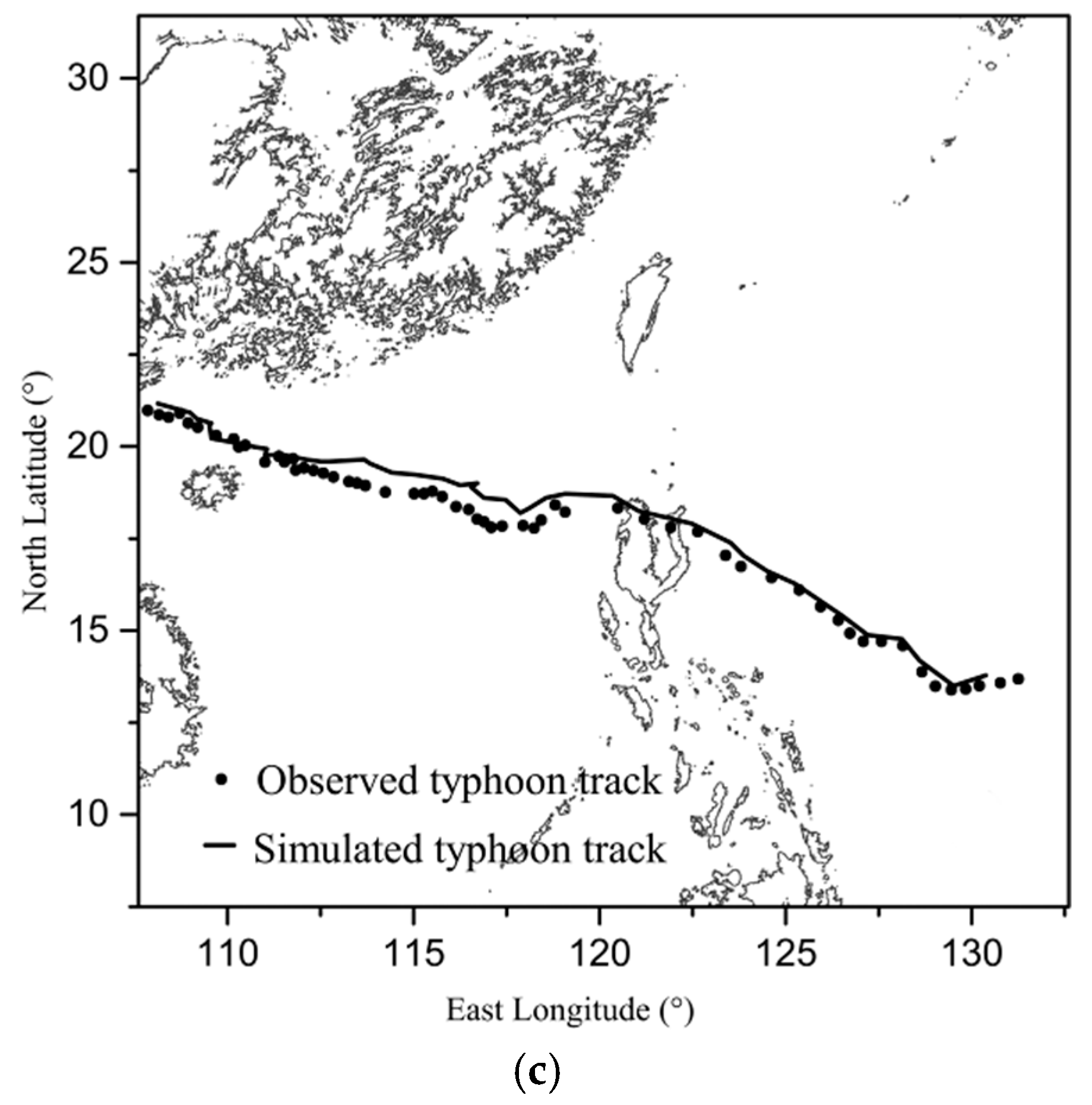
The tracks of the three typhoons, extracted from both the public data and simulation results, under investigation are presented in Figure 3. It is figuratively evident that the simulated tracks are close to the tracks extracted from the public data. In fact, the most significant deviation is observed for the typhoon Matmo (Figure 3b) near the sea shore, which is only ~2° in terms of longitude and latitude differences. Considering that the error buried in the authority-published tracks can reach the maximum value of 6.53° [42], the deviation of ~2° substantiates that the simulation results are reliable in terms of reproducing the large-scale meteorological features of a typhoon.

3.5.2. Local Features

In addition to the large-scale features, the time series of wind speeds and directions measured by the buoys are compared to the corresponding simulation results. The simulated wind speeds at the lowest level (4 m) are extrapolated to have the wind speed at 3 m using cubic spline interpolation scheme [43]. Figure 4 shows the comparison of wind speeds and directions for the Dongchong buoy.

The comparisons corresponding to other buoys reveal similar patterns and therefore are omitted in the present paper for the sake of concise. It is evident from the figure that the simulated and observed wind speeds and directions are in good agreement. More importantly, the simulation results vary following the trend of observed values. Such agreement shown in Figure 4 substantiates the use of simulation results to investigate local features of the typhoon wind field. The observed wind speeds and directions are also used to validate the simulation results of the normal day cases. Figure 5 presents the comparisons similar to Figure 4 but corresponding to the normal day simulations (1 April to 8 April and 29 August to 5 September in 2014). Figure 4 and Figure 5 reveal that the simulation results of wind speeds and directions under the non-typhoon condition are close to the actual observations.

3.5.3. Error Statistics

Although Figure 4 and Figure 5 figuratively show that the simulations of both typhoon and non-typhoon wind fields are reliable enough to be employed in the investigation concerning the general wind characteristics over the South China Sea, a detailed error statistics report would be beneficial to assess, in quantitative sense, how close the simulation results are to the observational data. In fact, four indicators, namely the root mean square error (RMSE), the Bias, the SD error and the scatter index (SI), are selected to show the deviations of numerical simulation results from the observed values. The definitions of the four indicators are:

$$RMSE=\sqrt{{\displaystyle \sum _{i=1}^N{\left(S_i-O_i\right)}^2}/N}$$

(6)

$$Bias={\displaystyle \sum _{i=1}^N\left(S_i-O_i\right)}/N$$

(7)

$$SD=RMS{E}^2-Bia{s}^2$$

(8)

$$SI=RMSE/\overline{O}$$

(9)

In Equations (6)–(9), $S_i$ is the i th simulated wind speed/direction in a time series, $O_i$ is the corresponding observed value, $N$ is the total number of the samples, and the overbar indicates the calculation of arithmetic mean. It is noted that the simple arithmetic subtraction does not yield the difference between simulated and observed wind directions. Following Ferreira et al. [44] and Carvalho et al. [45], the difference between the simulated and observed wind direction is calculated as:

$$\begin{array}{cc}{S}_i-O_i={\mathsf{\theta }}_s-{\mathsf{\theta }}_o\left[\left(1-360\right)/\left|{\mathsf{\theta }}_s-{\mathsf{\theta }}_o\right|\right],& \mathrm{if} |{\mathsf{\theta }}_s-{\mathsf{\theta }}_o|>{180}^{°}\end{array}$$

(10)

According to the definitions of error indicators shown above, RMSE shows the deviation, in general, of the simulation result from the observed value. It should be noted that RMSE is sensitive to the extremes buried in the time series. The Bias is employed to assess the trend of the deviation. If the Bias is positive, the simulation value is generally higher than the observed corresponds and vice versa. The SD is the indicator showing the stability of the deviation. If the SD is low, it means that the difference between the simulated and observed values is stable in time. In such cases, the difference can be offset by a constant. More importantly, the low SD implies that the simulation captures the variations of the observed wind speed/direction and therefore the physics are truthfully simulated in the WRF model. The SI, on the other hand, shows the degree of dispersion. The four error indicators, corresponding to both typhoon and non-typhoon simulation cases, are summarized in

Table 4. Summary of the error indicators for the Typhoon Rammasun simulation. RMSE: root mean square error; SD: standard deviation; and SI: scatter index.

Observations	Data	RMSE	Bias	SD	SI
Dongchong Buoy	U10 (m·s−1)	2.4673	1.4396	2.0037	0.3744
	Θ (°)	66.2257	29.7893	59.1476	0.3059
Dameisha Buoy	U10 (m·s−1)	3.5856	3.0389	1.9030	0.7978
Wankou Buoy	U10 (m·s−1)	3.3802	2.6128	2.1445	0.5398
	Θ (°)	44.5392	17.8909	40.7879	0.4815

,

Table 5. Summary of the error indicators for the Typhoon Matmo simulation.

Observations	Data	RMSE	Bias	SD	SI
Dongchong buoy	U10 (m·s−1)	2.2162	−0.0055	2.2162	0.5362
	Θ (°)	124.0050	49.2884	113.7889	0.5781
Dameisha buoy	U10 (m·s−1)	2.0923	0.7071	1.9692	0.6927
Wankou buoy	U10 (m·s−1)	2.7150	0.5553	2.6576	0.7422
	Θ (°)	80.8182	25.4020	76.7223	0.3376

,

Table 6. Summary of the error indicators for the Typhoon Kalmaegi simulation.

Observations	Data	RMSE	Bias	SD	SI
Dongchong buoy	U10 (m·s−1)	2.3481	−0.7849	2.2130	0.3489
	Θ (°)	55.9161	−9.5200	55.0997	0.2718
Dameisha buoy	U10 (m·s−1)	2.3735	0.5253	2.3147	0.4273
Xiasha buoy	U10 (m·s−1)	2.7535	1.0735	2.5356	0.6547
	Θ (°)	82.8695	30.0231	77.2397	0.9545

,

Table 7. Summary of the error indicators for the simulations from 1 to 8 April 2014.

Observations	Data	RMSE	Bias	SD	SI
Dongchong buoy	U10 (m·s−1)	2.3959	0.1236	2.3927	0.3770
	Θ (°)	62.0364	−11.0630	61.0420	0.6883
Dameisha buoy	U10 (m·s−1)	2.4047	1.0788	2.1491	0.7551
	Θ (°)	80.4156	28.5225	75.1873	0.8923
Xiasha buoy	U10 (m·s−1)	3.4768	2.8724	1.9589	1.7093
	Θ (°)	84.3856	−47.1123	69.3263	0.6774

and

Table 8. Summary of the error indicators for the simulations from 29 August to 5 September 2014.

Observations	Data	RMSE	Bias	SD	SI
Dongchong buoy	U10 (m·s−1)	1.4658	0.4717	1.3879	0.4584
	Θ (°)	122.7804	24.2954	130.3526	0.5447
Dameisha buoy	U10 (m·s−1)	1.1662	0.0342	1.1657	0.4431
	Θ (°)	122.6387	37.5044	116.7633	1.1158
Wankou buoy	U10 (m·s−1)	2.7860	1.1100	2.5554	0.8653
	Θ (°)	83.9581	17.8758	82.0330	0.5021

.

Table 4, Table 5, Table 6, Table 7 and Table 8 show how the simulated wind speed/direction compares to the observations in addition to Figure 4 and Figure 5. The assessment of the WRF simulation of wind speeds has been reported by Wang and Jin [46], who used the abovementioned error indicators to show the reliability of WRF simulation results. Based on their criteria, the simulation of wind speeds could be assessed as “good” when the following requirement is met: (a) RMSE lower than 5.0 (RMSE < 5.0) or (b) SI lower 1.0 (SI < 1.0). Following their philosophy, it is evident that the simulation of wind speeds reported in the present study is generally in “good” agreement with the observed wind speeds except for one case in Table 7. In detail, the SI equals to 1.7093 in Table 7 for the observations obtained from the Xiasha buoy. The error indicators in other 14 comparisons, on the other hand, are lower than the criteria with the averaged RMSE equals to 2.6571 and averaged SI equals to 0.5151. A sensitivity analysis concerning the WRF simulation of high-wind-speed meteorological processes [45] shows that the RMSE of ~3 m·s⁻¹ implies reliable simulation results. Considering the RMSE values shown in Table 4, Table 5, Table 6, Table 7 and Table 8, it can be asserted that the simulated wind speeds at the 3 m level in the present study are reliable in most cases. In fact, the Bias stays in the range of (−1 m·s⁻¹, 1 m·s⁻¹) for most cases under investigation, except for the Typhoon Rammasun case (1.44 m·s⁻¹). The SD, on the other hand, is about 2 m²·s⁻² for all the comparisons under investigation. The wind direction simulations, on the other hand, are not as accurate as the wind speed simulations. It is argued that the resolution of the terrain model employed in the WRF simulation is the reason for the differences found in comparing the observed and simulated wind directions. In detail, since the observations are obtained close to the shore, the land topographies along the shore significantly impact the simulation of the wind field, especially the spatial variation of wind directions. The terrain model employed in the WRF simulation has a resolution of only 30 km × 30 km, which could lead to the unrealistic simulation of the land topography influence.

3.5.4. The Simulation Reliability

Although the error indicators show the accuracy and reliability of wind speed/direction simulations at the 3 m height, the simulation results of wind fields at higher levels are still in doubt. In addition, the buoy data is only available for validating simulation results in two seasons, and therefore the seasonal variation simulated by the WRF model has not been comprehensively validated. Fortunately, the historical re-analysis dataset with relatively high horizontal resolutions of 27 km × 27 km developed by European Centre for Medium-Range Weather Forecasts (ECMWF: http://www.ecmwf.int) is available for the authors to conduct a verification check, which could assess the simulation reliability of not only the wind speeds at higher altitudes but also the seasonal variations.

The ECMWF data, containing the wind fields at 26 pressure layers (from 10 hPa to 1000 hPa), is available four times a day (at 00, 06, 12 and 18 UTC, respectively). Although the ECMWF data is primarily produced by a global/regional meteorology model, the observational data obtained from the weather station network around the globe is employed to adjusted the model output after the quality-check. Therefore, the comparison between WRF simulation results and the ECMWF data verifies the WRF simulation results. The time stamp of the ECMWF dataset is checked to ensure only the datasets temporally consistent with the simulation periods (in both typhoon and non-typhoon cases) are downloaded from the online database. The wind profiles within the offshore area of the outmost domain D01 are extracted from the downloaded ECMWF dataset. Due to the relatively coarse resolution of the ECMWF data, the WRF simulated wind profiles at the same locations as the ECMWF data can be selected from the simulation results. Using the wind speeds, extracted from the ECMWF dataset and produced by the WRF simulation, at heights below 1600 m, the values of RSME and SI at various heights corresponding to each of the simulation periods and ECMWF grid points are calculated according to Equations (6) and (9). For the three typhoon simulations, the RSME and SI are then averaged horizontally to show the overall reliability of the simulation results. For the simulation of non-typhoon cases, the values of RMSE and SI corresponding to the same season are averaged horizontally, which produces the averaged RMSE and SI for each season at each height. Furthermore, considering the presence of land-sea transitions in D03A, the ECMWF data, which is primarily produced by a global model, may fail to grasp the effects of transitions on cross-boundary wind fields while the WRF simulation is supposed to reasonably model the wind fields in such a case when the high-quality topography (30 arc-second) is input. Therefore, deviations between ECMWF-extracted and WRF simulated wind speeds, are expected along the coastline in D03A. Such deviations, which indeed show the inadequacy of the ECMWF data, should be distinguished and excluded from the calculation of RMSE and SI. Therefore, the land/sea indicator contained in the static WRF data is referenced. More specifically, the land/sea indicators (corresponding to 2 × 2 grid points) surrounding a given ECMWF grid point are checked labeled as land-sea transition point if the indicators imply both the land and sea types. The RMSEs corresponding to the land-sea transition points and the offshore points are then calculated separately.

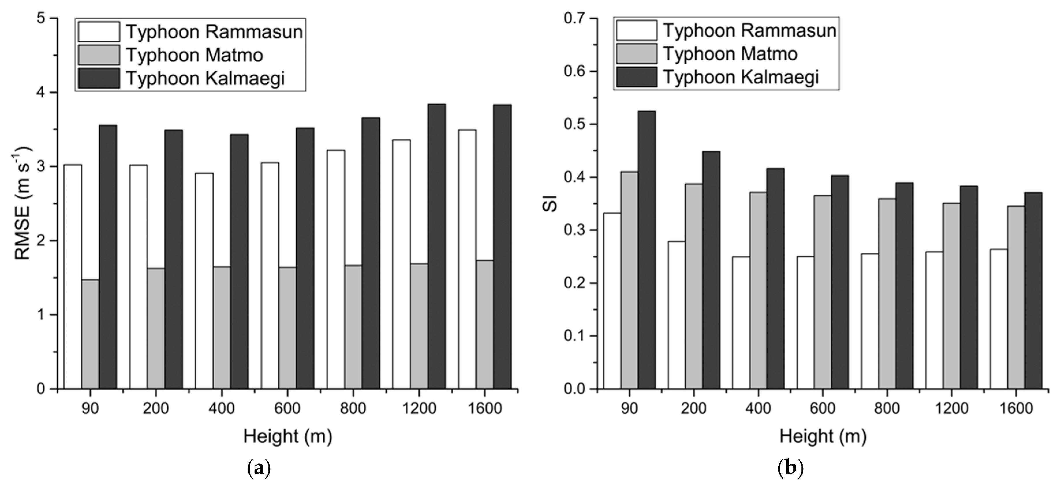
Figure 6 presents the error indicators in the three typhoon simulations, which shows the differences between the simulated and ECMWF-extracted wind speeds before and after typhoons making landfalls. The maximum RMSE and SI appear in Typhoon Kalmaegi case, which are ~3.6·m·s⁻¹ and ~0.42, respectively. In general, the performances of simulations are good according to the criteria suggested by Wang and Jin [46]. It should be noted that, both indicators only slightly increase with heights, which verifies that the simulation results at altitudes higher than 3 m are acceptable.

The averaged RMSE corresponding to the land-sea transition and offshore points are calculated in Figure 7. It is obvious that the deviations (~2.87 m·s⁻¹) between the ECMWF-extracted and WRF simulated wind speeds corresponding to the transition points are larger than the RMSE corresponding to the offshore area (~2.34 m·s⁻¹). The maximum deviation with the RMSE of ~4.52 m·s⁻¹ appears in Typhoon Kalmaegi case at the level of 90 m. Since the sea-land wind field transition, which relies heavily on the geometries of the costal lines, plays an important role in influencing the wind field near the shore, especially at the lower altitudes, the comparison of deviations shown in Figure 7 follows the expectation because of the resolution (27 km × 27 km) of the terrain topographies implied by the ECMWF data.

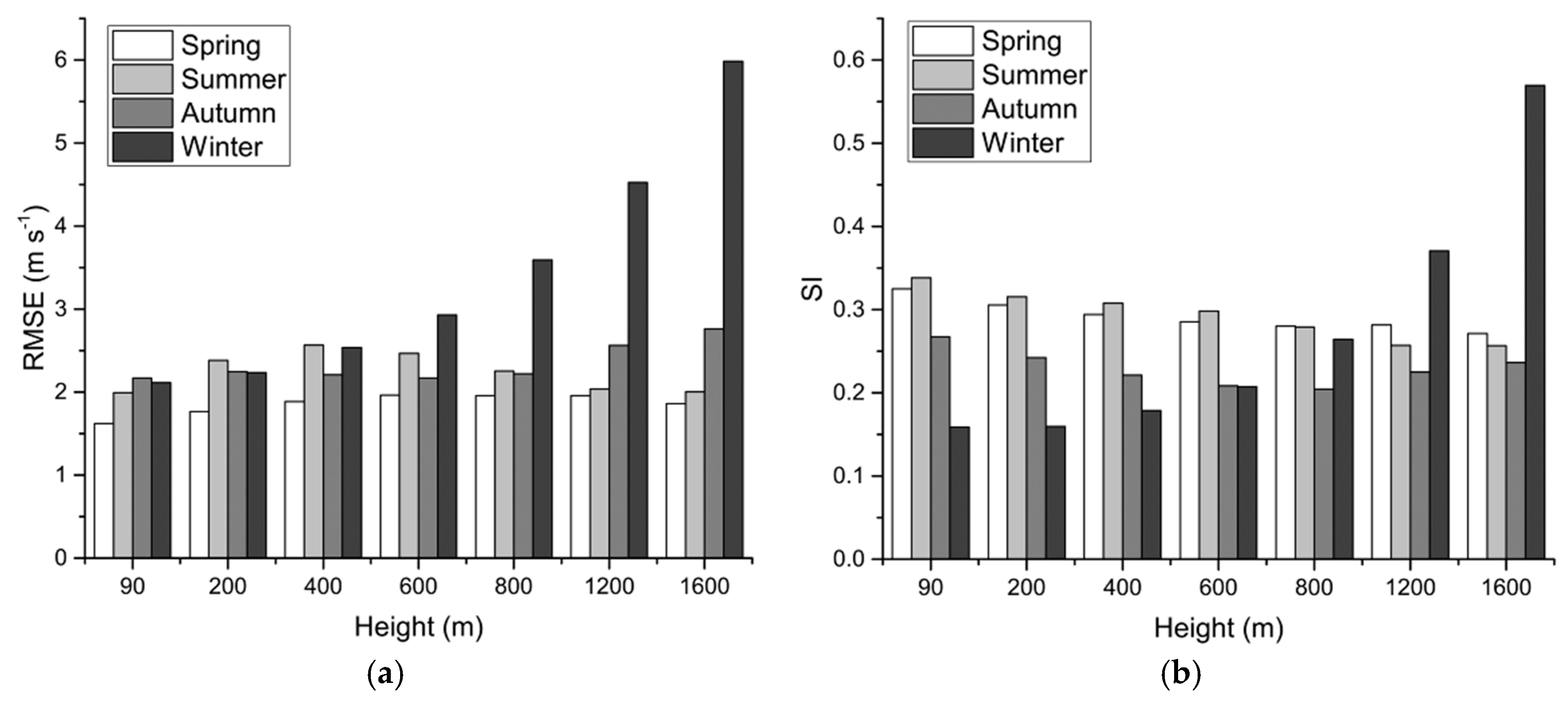
Figure 8 shows the error indicators exhibiting the differences between the simulated and ECMWF-extracted wind speeds under normal conditions in different seasons of the year 2005. The maximum deviation appears for the winter simulation, especially at the highest level of 1600 m with ~6 m·s⁻¹ for RMSE and ~0.6 for SI. Similar patterns are observed when investigating the simulation reliability in the other eight years. The effect of seasonal variations on WRF simulated wind speeds are discussed by Li et al. as well [47], who also concluded that the maximum errors are found in winter simulations. Furthermore, the complex atmospheric dynamics and the lack of direct observations at higher altitudes make the high-level simulation unrealistic. Therefore, the simulation results at heights exceeding 400 m in winter may be not reliable. Still, the simulated wind speeds are acceptable at lower levels (<400 m).

Except for winter, the effects of seasonal variations on simulation results are relatively weak and the error indicators roughly remain constants (~2.5 m·s⁻¹ for RMSE and ~0.3 for SI) for different seasons. In addition, the errors increase with heights as shown in Figure 8, which is consistent with the conclusions drawn by previous scholars [46,48].

Figure 9 shows the averaged RMSE for land-sea transition points (~2.35 m·s⁻¹) and offshore area (~2.13 m·s⁻¹), similar with the typhoon cases in Figure 7. Both the maximum deviations appear in winter season with the maximum RMSEs of ~6.03 m·s⁻¹ at 90 m and ~6.17 m·s⁻¹ at 1600 m level. Considering the WRF simulation along the coastline including the influence of high-quality topography, it is evident from the figure that while the deviation corresponding to the offshore area increase with heights, the deviation corresponding to the land-sea transition point yield the maximum deviation at the level of 90 m. It is argued that the differences between Figure 9a,b should be attributed to the reliability and accuracy of the terrain topographies. Generally speaking, the WRF simulation is better in terms of predicting the wind field along the coastline. Therefore, the deviations shown in Figure 7a and Figure 9a should not be interpreted as the inadequacy of the WRF simulation.

It should be noted that the comparisons shown in Figure 6, Figure 7, Figure 8 and Figure 9 are merely verifications, rather than validations, of the WRF simulation results because the ECMWF data is essentially numerical model outputs. Nevertheless, the agreements shown in Figure 6, Figure 7, Figure 8 and Figure 9 indicate that the WRF simulation contained in the present study is trustworthy as it produces results in line with the widely-acknowledged ECMWF data. Validations of the WRF simulation results based on direct field measurements are, however, still necessary to substantiate the use of WRF simulation results to investigate wind field above the atmospheric surface layer, and therefore such validations are the topic for the future work of the authors.

In conclusion, although the simulation results deviate from the ECMWF data with the increasing height, such deviation is acceptable below 400 m. In addition, the ECMWF data itself could be erroneous, such as in the cross-boundary wind field along the coastline. Moreover, based on the decent accuracy of the simulations that validated by buoy observations near the sea level, the use of the simulation results in deriving an engineering wind profile model below the height of regular wind turbines (~100 m) for the purpose of calculating the wind load is justified.

4. Discussion on the Engineering Model

To assess validity of the power-law and log-law model in terms of describing the vertical variation of wind speeds over the South China Sea, the wind profiles extracted from the WRF simulations are averaged and compared to the calculations made according to both the power-law and log-law model. In the power-law model, the Hellmann exponent $\mathsf{\alpha }$ is the main parameter determining the shape of the wind profile. In the log-law model, the friction velocity $u_{*}$ is the critical parameter when combining the Equation (2) with the Charnock assumption (Equation (3)). Thus, the discussion focuses on both the formulae and the main parameters used in the two models.

4.1. Typhoon Condition

As discovered by Zhang et al. [49], the stability of the typhoon boundary layer is near-neutral, which means that its turbulence processes are dominated by the dynamic mechanism. Therefore, the atmospheric stability of the wind profiles extracted from the WRF simulation results should be checked to eliminate the profiles under only weak typhoon influences. According to the relations between the bulk Richardson number and the mean boundary layer (MBL) wind, as shown in Tse et al.’s work [50], the extracted mean wind profiles whose wind speed at 10 m exceeding 12 m·s⁻¹ is for certain of the near-neutral stability. Moreover, it is reasonable to assume that the wind strength, indicated by the mean wind speed at 10 m, impacts the shape of the typhoon boundary layer mean wind profile. Consequently, the mean wind speed at 10 m ($U_{10}$) interpolated from the resulting mean wind profiles derived from post-processing the WRF simulation results is checked and the resulting mean wind profiles are binned according to $U_{10}$ with a step size of 4 m·s⁻¹ (12–16 m·s⁻¹, 16–20 m·s⁻¹, 20–24 m·s⁻¹ and 24–29 m·s⁻¹). The number of profiles belonging to each bin is 345, 74, 28 and 15.

When normalizing by the simulated wind speed at lowest elevation of 4 m, the resulting mean wind profiles belonging to each bin can be compared to the calculations made according to the power-law and log-law model. For the parameter $\mathsf{\alpha }$ in the power-law model, the value of 0.11 as suggested by DNV for extreme condition is adopted. For log-law model, the friction velocity $u_{*}$ is calculated according to the formulae provided by the code [23]. Figure 10 presents the comparisons. It is evident from the figure that both models overestimate the wind speed for the heights exceeding 80 m when U₁₀ < 20 m·s⁻¹. Along with the increase of wind strength, the calculations made according to both models become close to the resulting mean wind profile.

It has been found from the figures that neither the power-law model nor the log-law model is sufficiently accurate when describing the vertical variation of wind speeds over the South China Sea under the typhoon condition. In particular, the parameters (such as $\mathsf{\alpha }$ in the power-law model), which are assumed to be constant regardless of the wind strength, has been found vary with $U_{10}$. In fact, it has been discerned that the slope of the wind profile near the sea surface, which implies the magnitudes of the model parameter ($\mathsf{\alpha }$ or $u_{*}$), decreases with the increasing wind strength. Figure 10 includes the tangent lines of the bin-representative profile calculated by averaging the resulting mean wind profile belonging to a single bin. The tangent lines figuratively show the decrease of profile slope near the sea surface, and hence the increases of $\mathsf{\alpha }$ or $u_{*}$, with the increasing $U_{10}$. When the wind strength, revealed by $U_{10}$, increases, the performance of both the power-law and the log-law model improves. For the resulting mean wind profiles within the last bin ($U_{10}$ varied from 24 m·s⁻¹ to 29 m·s⁻¹), the model profiles, calculated according to either the power-law or the log-law, acceptably capture the vertical variation of wind speeds. To be more illustrative, the RMSE and the Bias between the model predictions and the resulting mean wind profiles are calculated. Figure 11 presents the variations of the RMSE and the Bias, corresponding to every single resulting mean wind profile, with $U_{10}$.

Based on the findings articulated above, it is postulated that both the power-law and the log-law models are applicable to describe the vertical variation of typhoon wind speeds over the South China Sea under the condition that the model parameters, such as $\mathsf{\alpha }$ and $u_{*}$, are revised to vary with $U_{10}$. When the heights and wind speeds from the resulting mean wind profiles are logarithmically scaled in a proper way, a linear regression process can be applied to find the best fitted $\mathsf{\alpha }$ and $u_{*}$ for each of the resulting mean wind profiles. Figure 12 plots the best fitted $\mathsf{\alpha }$ and $u_{*}$ against $U_{10}$.

From Figure 12, it is found that: (a) a logarithmic function is suitable for describing the variation of $\mathsf{\alpha }$ with $U_{10}$ and (b) $u_{*}$ increases with $U_{10}$ in the approximate linear sense. Consequently, linear regression is once again employed to determine the relationship between $\ln (U_{10})$ and $\mathsf{\alpha }$, $U_{10}$ and $u_{*}$. The regression results show:

$$\mathsf{\alpha }=-0.0808+0.0556\ln \left(0.5946+U_{10}\right)$$

(11)

$$u_{*}=0.0636\cdot U_{10}-0.4630$$

(12)

When substituting Equations (11) and (12) into (1) and (4), the power-law and log-law models are revised to provide more reliable estimates of wind speeds in the typhoon boundary layer over the South China Sea. It should be noted that, both the revised formulae take $U_{10}$ as the solo input parameter. Given the value of $U_{10}$, Equations (1) and (4), with the auxiliary parameters calculated by Equations (11) and (12), fully determine the vertical variation of wind speeds.

4.2. Non-Typhoon Condition

Following the steps articulated in Section 4.1, the resulting mean wind profiles corresponding to the normal day simulations are calculated. Different from the discussion concerning the wind profile under the typhoon condition, the scheme to bin resulting mean wind profiles is no longer based on $U_{10}$ in the normal-day cases. Instead, the Obukhov length scale, which shows the atmospheric stability quantitatively, is employed as the indicator to bin the resulting mean wind profiles. The Obukhov length scale [51] is calculated as:

$$L=-\left(T{u}_{*}^3\right)/\left[g{K}_a\cdot \left(\overline{wT}\right)\right]$$

(13)

In Equation (13), $T$ is the mean virtual potential temperature, $w$ is the vertical wind speed and hence $\left(\overline{wT}\right)$ calculates the total heat flux. In fact, the inverse Obukhov length scale, i.e., L⁻¹, is commonly used to indicate the atmospheric stability. Following the classification scheme adopted by Drew et al. [52], the unstable, near-neutral and stable atmospheric boundary layer is identified with L⁻¹ in the ranges of −10–−0.1 m⁻¹, −0.1–0.1 m⁻¹ and 0.1–10 m⁻¹ respectively. The resulting mean wind profiles with L⁻¹ < −10 m⁻¹ and L⁻¹ > 10 m⁻¹ are thrown away which make the number of the resulting mean wind profile available for further analysis reduced from 8040 to 5246.

Figure 13 presents the wind profiles corresponding to near-neutral stability, while Figure 14 shows the wind profiles corresponding to unstable stability and stable stability (labeled as hollow squares). It can be observed from the figures that the slope of the bin-representative profile at lower altitudes (<100 m) increases when the atmospheric stability moves from unstable state to the stable state. Such findings are in line with the conclusions derived by Clobes et al. [53], who classified different profile shapes from 16,418 observed wind profiles using artificial neural network method. In addition, the experiments conducted by Muñoz [54] also show the similar features for the wind profiles under the influence of different atmospheric stabilities.

As regards the engineering models describing the wind profiles shown in Figure 13 (labeled as hollow squares), both the power-law and the log-law models are widely acknowledged as valid in the near-neutral stratification. In the non-typhoon cases, the wave heights, and hence the parameters ($\mathsf{\alpha }$ and $u_{*}$) which show the influence of surface roughness, are independent from the wind strength as the wind speed is low. Given that both $\mathsf{\alpha }$ and $u_{*}$ are constant, the linear regression can be employed to determine the best fitted $\mathsf{\alpha }$ and $u^{*}$ for the near-neutral boundary layer over the South China Sea. The linear regression results show that, $\mathsf{\alpha }=0.0640$ and $u_{*}$ = 0.4186 m·s⁻¹. The bin-representative profile corresponding to the near-neutral stability is compared to power-law and log-law models in Figure 13.

It is evident from the figure that the power-law model outperforms the log-law model in terms of describing the vertical variation of wind speeds below 300 m. In fact, the log-law profile deviates from the bin-representative profile below 150 m, but the deviation reduces with the increasing height. In general, the log-law model predications are acceptable above 90 m.

When the atmospheric boundary layer is stable or unstable, neither the log-law nor the power-law model is considered sufficient to show the vertical variation of wind speeds. The log-law model has been, however, adopted by previous scholars [55,56] as the base for modification to calculate both the stable and unstable wind profiles. Therefore, it is proposed that the logarithmic function with a simple correction term may be suitable for describing wind profiles under the influence of appreciable atmospheric stabilities. In fact, it is postulated that the log-law profile model can be revised as:

$$U(h)=\left(u_{*}/K_a\right)\cdot \left[\ln \left(h/z_0\right)-{\mathsf{\Psi }}_m\left(h/L\right)\right]$$

(14)

The term ${\mathsf{\Psi }}_m$ in Equation (14) is a function to be determined, which counts for the influence of the atmospheric stability. Through a trial-error process, it has been found that an exponential form of ${\mathsf{\Psi }}_m$ leads to the profile calculated according to Equation (14) sufficiently approximating the bin-representative profiles shown in Figure 14. In fact, it is proposed that:

$${\mathsf{\Psi }}_m=a\cdot {\left|h/L\right|}^b$$

(15)

This leads to the profile model expressed as:

$$U\left(h\right)=\left(u_{*}/K_a\right)\cdot \left[\ln \left(h/z_0\right)+a\cdot {\left|h/L\right|}^b\right]$$

(16)

As introduced in Equation (2), $u_{*}$ is the friction velocity while $K_a$ is the von Karman constant, equaling to 0.4, $h$ is the height from the ground/sea surface, $z_0$ is the roughness length and L is the Obukhov length scale. When comparing the Equation (16) to the bin-representative profile corresponding to both the stable and unstable stratifications, the parameters of $a$, $b$ and $z_0$ are derived through a nonlinear fitting process. In detail, the Levenberg-Marquardt algorithm [57,58], an elegant optimization method to solve the nonlinear least squares problem, is used to do the nonlinear fitting. The results show that, $a=-0.8196$, $b=0.2269$, $u_{*}$ = 0.3635 m·s⁻¹ for the stable stratification, and $a=-0.5210$, $b=0.2753$, $u_{*}$ = 0.2005 m·s⁻¹ for the unstable stratification. After the log-law model is revised and the best-fitted parameters are included, model predictions are compared to the bin-presentative profiles in Figure 14.

It is clear from the figure that, the profiles calculated according to the revised log-law model are in good agreement with the bin-representative profile at lower altitudes (4–300 m). The bin-representative profiles, however, deviate the model predictions at heights exceeding 300 m. In fact, under both stable and unstable conditions, the model calculations underestimate the wind speeds above 300 m. One plausible explanation concerns the turbulent exchanges of momentum above 300 m is too complicated to be modelled by Equation (16), which in turn makes the revised log-law model inapplicable to describe the vertical variation of wind speeds exceeding the height of 300 m.

In summary, while the power-law and the log-law models with the parameters of 0.0640 for $\mathsf{\alpha }$, 0.4186 m·s⁻¹ for $u_{*}$ are valid to describe the wind profile over the South China Sea in a neutrally stratified atmospheric boundary layer under non-typhoon conditions, the log-law model with simple exponential modification can be considered sufficient to show the wind profile in normal days over the South China Sea under the stable and unstable stratification.

5. Conclusions

Through numerically simulating the wind field over several potential sites for constructing the floating wind farms in the South China Sea, the present paper discusses the engineering models applicable to describe the vertical variation of wind speeds in potential wind farms under both typhoon and non-typhoon conditions. Through validating based on buoy measurements and verifying based on the widely-acknowledged ECMWF data, the numerically simulated wind field is found reliable for a discussion on the wind field over the South China Sea below 400 m.

For the wind field under the typhoon condition, it has been found that both the power-law model and the log-law model could be valid to show the mean wind profile in the South China Sea typhoon boundary layer given the model parameters revised to vary with the wind strength. In fact, a model (Equations (11) and (12)) is proposed to estimate the value of $\mathsf{\alpha }$ and $u_{*}$ according to $U_{10}$ in the present paper.

For the wind field under the non-typhoon condition, it is suggested that the atmospheric stability should be included in the wind profile model. In detail, for the near-neutral stability, the conventional power-law model has been found suitable to show the wind profile below 300 m. In the height range of 150 m to 400 m, both models (the power-law model and the log-law model) are equally valid to calculate the near-neutral wind profile. For stable and unstable stratification, a simple exponential correction is suggested to be included in the log-law model in the calculation of the stable and unstable wind profile over the South China Sea. Two parameters are introduced to adjust the exponential correction, whose values, corresponding to the stable and unstable stratification respectively, are derived through a nonlinear fitting process to show the atmospheric stability influence.

References

1. EWEA Business Intelligence. Aiming High Rewarding Ambition in Wind Energy; The European Wind Energy Association: Brussels, Belgium, 2015. [Google Scholar]
2. Liu, Y.; Li, S.; Yi, Q.; Chen, D. Developments in semi-submersible floating foundations supporting wind turbines: A comprehensive review. Renew. Sustain. Energy Rev. 2016, 60, 433–449. [Google Scholar] [CrossRef]
3. Failla, G.; Arena, F. New perspectives in offshore wind energy. Philos. Trans. R. Soc. Lond. A Math. Phys. Eng. Sci. 2015, 373, 20140228. [Google Scholar] [CrossRef] [PubMed]
4. Global Wind Statistics 2015; Global Wind Energy Council: Brussels, Belgium, 2016.
5. Heronemus, W.E. Pollution-Free Energy from the Offshore Winds; Marine Technology Society: Washington, DC, USA, 1972. [Google Scholar]
6. Zheng, C.; Zhuang, H.; Li, X.; Li, X. Wind energy and wave energy resources assessment in the East China Sea and South China Sea. Sci. China Technol. Sci. 2011, 55, 163–173. [Google Scholar] [CrossRef]
7. Douglas, P.H. The development of a system of federal grants-in-aid II. Political Sci. Q. 1920, 35, 522–544. [Google Scholar] [CrossRef]
8. Shao, L. The Evolution of Sea Wave and Sea Level; China Institute of Navigation: Dalian, China, 2003. (In Chinese) [Google Scholar]
9. Liang, S.X.; Sun, Z.C.; Yin, H.Q.; Niu, H.Y. Influence Factors of Typhoon Wave Forecast in the South Sea by SWAN Model. Adv. Mar. Sci. 2015, 33, 19–30. (In Chinese) [Google Scholar]
10. Choi, E.C. Field measurement and experimental study of wind speed profile during thunderstorms. J. Wind Eng. Ind. Aerodyn. 2004, 92, 275–290. [Google Scholar] [CrossRef]
11. Wilson, B.W. Numerical prediction of ocean waves in the North Atlantic for December, 1959. Deutsch. Hydrogr. Z. 1965, 18, 114–130. [Google Scholar] [CrossRef]
12. Paik, J.K.; Faulkner, D. Reassessment of the MV derbyshire sinking with the focus on hull-girder collapse. Mar. Technol. 2003, 40, 258–269. [Google Scholar]
13. Li, L.; Kareem, A.; Xiao, Y.; Song, L.; Qin, P. Wind Profile and Spectra in Typhoon-Prone Regions in South China. In Proceedings of the Advances in Hurricane Engineering Conference, Miami, FL, USA, 24–26 October 2012; pp. 929–940.
14. Hsu, S. Verifying Wind Profile Equations Under Hurricane Conditions. Open Ocean Eng. J. 2011, 4, 60–64. [Google Scholar] [CrossRef]
15. Giammanco, I.M.; Schroeder, J.L.; Powell, M.D. Observed characteristics of tropical cyclone vertical wind profiles. Wind Struct. 2012, 15, 65–86. [Google Scholar] [CrossRef]
16. Ames, D.P.; Quinn, N.W.; Rizzoli, A.A. Relationship between Von Karman and Reynolds number: A critical analysis using the wind profile method. In Proceedings of the 7th International Congress on Environmental Modelling and Software: Bold Visions for Environmental Modeling (iEMSs 2014), San Diego, CA, USA, 15–19 June 2014.
17. Guide for Building and Classing Offshore Wind Turbine Installation; American Bureau of Shipping (ABS): Houston, TX, USA, 2014.
18. Design of Offshore Wind Turbine Structures; DNV-OS-J101; Det Norske Veritas: Høvik, Norway, 2014.
19. Counihan, J. Adiabatic atmospheric boundary layers: A review and analysis of data from the period 1880–1972. Atmos. Environ. (1967) 1975, 9, 871–905. [Google Scholar] [CrossRef]
20. Bañuelos-Ruedas, F.; Angeles-Camacho, C.; Rios-Marcuello, S. Analysis and validation of the methodology used in the extrapolation of wind speed data at different heights. Renew. Sustain. Energy Rev. 2010, 14, 2383–2391. [Google Scholar] [CrossRef]
21. Wind Turbines—Part 3: Design Requirements for Offshore Wind Turbines; No. IEC61400-3; International Electrotechnical Commission: Geneva, Switzerland, 2009.
22. Hsu, S.A.; Meindl, E.A.; Gilhousen, D.B. Determining the Power-Law Wind-Profile Exponent under Near-Neutral Stability Conditions at Sea. J. Appl. Meteorol. 1994, 33, 757–765. [Google Scholar] [CrossRef]
23. Environmental Conditions and Environmental Loads; DNV-RP-C205; Det Norske Veritas: Høvik, Norway, 2010.
24. Charnock, H. Wind stress on a water surface. Q. J. R. Meteorol. Soc. 1955, 81, 639–640. [Google Scholar] [CrossRef]
25. Michalakes, J.; Dudhia, J.; Gill, D.; Klemp, J.; Skamarock, W. Design of a Next-Generation Regional Weather Research and Forecast Model: Towards Teracomputing; World Scientific: River Edge, NJ, USA, 1998; pp. 117–124. [Google Scholar]
26. Grell, G.A.; Peckham, S.E.; Schmitz, R.; McKeen, S.A.; Frost, G.; Skamarock, W.C.; Eder, B. Fully coupled “online” chemistry within the WRF model. Atmos. Environ. 2005, 39, 6957–6975. [Google Scholar] [CrossRef]
27. Laprise, R. The Euler equations of motion with hydrostatic pressure as an independent variable. Mon. Weather Rev. 1992, 120, 197–207. [Google Scholar] [CrossRef]
28. The General Institute of Hydropower and Water Resource Planning and Design, Preparation Rule of Offshore Wind Power Projects Planning Report. 2008. Available online: www.doc88.com/p-6083742083777.html (accessed on 28 December 2016).
29. RA IV Hurricane Committee. Regional Association IV Hurricane Operational Plan 2015; World Meteorological Organization: Geneva, Switzerland, 2015. [Google Scholar]
30. Wang, W.; Bruyere, C.; Duda, M.; Dudhia, J.; Gill, D.; Lin, H.; Michalakes, J.; Rizvi, S.; Zhang, X.; Beezley, J. ARW Version 3 Modeling System User’s Guide. Mesoscale & Miscroscale Meteorology Division; National Center for Atmospheric Research: Boulder, CO, USA, 2010. [Google Scholar]
31. Takagi, H.; Wu, W. Maximum wind radius estimated by the 50 kt radius: Improvement of storm surge forecasting over the Western North Pacific. Nat. Hazards Earth Syst. Sci. Discuss. 2015, 3, 6431–6457. [Google Scholar] [CrossRef]
32. Kawai, H.; Honda, K.; Tomita, T.; Kakinuma, T. Characteristic of Typhoons in 2004 and Forecasting and Hindcasting of Their Storm Surges; Technical Note of the Port and Airport Research Institute: Yokosuka, Japan, 2005. [Google Scholar]
33. Paulson, C.A. The mathematical representation of wind speed and temperature profiles in the unstable atmospheric surface layer. J. Appl. Meteorol. 1970, 9, 857–861. [Google Scholar] [CrossRef]
34. Skamarock, W.C.; Klemp, J.B.; Dudhia, J.; Gill, D.O.; Barker, D.M.; Wang, W.; Powers, J.G. A Description of the Advanced Research WRF Version 3; Mesoscale and Microscale Meteorology Division, National Center for Atmospheric Research: Boulder, CO, USA, 2008; pp. 7–25. [Google Scholar]
35. Hong, S.-Y.; Pan, H.-L. Nonlocal boundary layer vertical diffusion in a medium-range forecast model. Mon. Weather Rev. 1996, 124, 2322–2339. [Google Scholar] [CrossRef]
36. Hong, S.; Lakshmi, V.; Small, E.E.; Chen, F.; Tewari, M.; Manning, K.W. Effects of vegetation and soil moisture on the simulated land surface processes from the coupled WRF/Noah model. J. Geophys. Res. Atmos. 2009, 114. [Google Scholar] [CrossRef]
37. Kain, J.S. The Kain-Fritsch convective parameterization: An update. J. Appl. Meteorol. 2004, 43, 170–181. [Google Scholar] [CrossRef]
38. Hong, S.-Y.; Dudhia, J.; Chen, S.-H. A revised approach to ice microphysical processes for the bulk parameterization of clouds and precipitation. Mon. Weather Rev. 2004, 132, 103–120. [Google Scholar] [CrossRef]
39. Mlawer, E.J.; Taubman, S.J.; Brown, P.D.; Iacono, M.J.; Clough, S.A. Radiative transfer for inhomogeneous atmospheres: RRTM, a validated correlated-k model for the longwave. J. Geophys. Res. Atmos. 1997, 102, 16663–16682. [Google Scholar] [CrossRef]
40. Specifications for Oceanographic Survey Part 3: Marine Meteorological Observations (GB/T12763.3-2007/8); State Oceanic Administration: Beijing, China, 2007. (In Chinese)
41. Knapp, K.R.; Kruk, M.C. Quantifying Interagency Differences in Tropical Cyclone Best-Track Wind Speed Estimates. Mon. Weather Rev. 2010, 138, 1459–1473. [Google Scholar] [CrossRef]
42. Hyekyeong, H.A.; Hui, W.Z.; Yun, K.J.; Jie, N.S.; Aesook, S. The impact of cumulus parameterizations and micro-physics schemes of different combinations on typhoon track prediction. J. Trop. Meteorol. 2009, 25, 435–441. [Google Scholar]
43. Mckinley, S.; Levine, M. Cubic Spline Interpolation. Numer. Math. J. Chin. Univ. 1999, 64, 44–56. [Google Scholar]
44. Ferreira, A.; Castanheira, J.; Rocha, A.; Ferreira, J. Estudo de Sensibilidade das Previsões de Superfície em Portugal Pelo WRF Face à Variação das Parametrizações Físicas. 2008. Available online: http://repositorio.aemet.es/bitstream/20.500.11765/5319/1/3A_Ferreira_2.pdf (accessed on 28 December 2016).
45. Carvalho, D.; Rocha, A.; Gómez-Gesteira, M.; Santos, C. A sensitivity study of the WRF model in wind simulation for an area of high wind energy. Environ. Model. Softw. 2012, 33, 23–34. [Google Scholar] [CrossRef]
46. Wang, C.; Jin, S. Error features and their possible causes in simulated low-level winds by WRF at a wind farm. Wind Energy 2013, 17, 1315–1325. [Google Scholar] [CrossRef]
47. Li, J.H.; Guo, Z.H.; Wang, H.J. Analysis of Wind Power Assessment Based on the WRF Model. Atmos. Ocean. Sci. Lett. 2014, 7, 126–131. [Google Scholar]
48. Sienkiewicz, M.J. Evaluation of WRF Planetary Boundary Layer Schemes over the Coastal Waters of Southern New England. Master’s Thesis, Stony Brook University, Stony Brook, NY, USA, 2014. [Google Scholar]
49. Zhang, J.A.; Drennan, W.M.; Black, P.G.; French, J.R. Turbulence Structure of the Hurricane Boundary Layer between the Outer Rainbands. J. Atmos. Sci. 2009, 66, 2455. [Google Scholar] [CrossRef]
50. Tse, K.T.; Li, S.W.; Chan, P.W. Wind profile observations in tropical cyclone events using wind-profilers and Doppler SODARs. J. Wind Eng. Ind. Aerodyn. 2013, 115, 93–103. [Google Scholar] [CrossRef]
51. Venkatram, A. Estimating the Monin-Obukhov length in the stable boundary layer for dispersion calculations. Bound.-Layer Meteorol. 1980, 19, 481–485. [Google Scholar] [CrossRef]
52. Drew, D.R.; Barlow, J.F.; Lane, S.E. Observations of wind speed profiles over Greater London, UK, using a Doppler lidar. J. Wind Eng. Ind. Aerodyn. 2013, 121, 98–105. [Google Scholar] [CrossRef]
53. Clobes, M.; Willecke, A.; Peil, U. Shape-dependent characteristics of full-scale wind profiles. J. Wind Eng. Ind. Aerodyn. 2011, 99, 919–930. [Google Scholar] [CrossRef]
54. Muñoz-Esparza, D.; Canadillas, B. Forecasting the diabatic offshore wind profile at FINO1 with the WRF mesoscale model. DEWI Mag. 2012, 40, 73–79. [Google Scholar]
55. Businger, J.A. A note on the Businger-Dyer profiles. Bound.-Layer Meteorol. 1988, 42, 145–151. [Google Scholar] [CrossRef]
56. Dyer, A. A review of flux-profile relationships. Bound.-Layer Meteorol. 1974, 7, 363–372. [Google Scholar] [CrossRef]
57. Levenberg, K. A method for the solution of certain non-linear problems in least squares. Q. Appl. Math. 1944, 2, 164–168. [Google Scholar] [CrossRef]
58. Marquardt, D.W. An algorithm for least-squares estimation of nonlinear parameters. J. Soc. Ind. Appl. Math. 1963, 11, 431–441. [Google Scholar] [CrossRef]
Figure 1. The weather research and forecast (WRF) domain configuration shown on top of the hydrology map of the South China Sea. 29 potential floating wind farm sites were indicated by small squares.
Energies 10 00125 g001
Figure 2. The comparisons of typhoon parameters derived from the numerical simulation results and public data during the passages of 3 typhoons: (a) maximum wind speed; and (b) central pressure.
Energies 10 00125 g002
Figure 3. The comparisons of observed and simulated typhoon tracks: (a) Typhoon Rammasun; (b) Typhoon Matmo; and (c) Typhoon Kalmaegi.
Energies 10 00125 g003aEnergies 10 00125 g003b
Figure 4. The comparisons between observed and simulated wind speed and direction at 3 m-elevation from 15 to 18 July, from 20 to 24 July and from 12 to 18 September in 2014: (a) the wind speed of Typhoon Rammasun; (b) the wind direction of Typhoon Rammasun; (c) the wind speed of Typhoon Matmo; (d) the wind direction of Typhoon Matmo; (e) the wind speed of Typhoon Kalmaegi; and (f) the wind direction of Typhoon Kalmaegi.
Energies 10 00125 g004aEnergies 10 00125 g004b
Figure 5. The comparisons between observed and simulated wind speed and direction at 3 m-elevation under normal conditions: (a) the wind speed from 1 to 8 April 2014; (b) the wind direction from 1 to 8 April 2014; (c) the wind speed from 29 August to 5 September 2014; and (d) the wind direction from 29 August to 5 September 2014.
Energies 10 00125 g005
Figure 6. The error indicators in the three typhoon simulations: (a) the RMSE; and (b) the SI.
Energies 10 00125 g006
Figure 7. The RMSE of the three typhoon simulations in land-sea transition and offshore area: (a) the land-sea transition; and (b) the offshore area.
Energies 10 00125 g007
Figure 8. The averaged mean wind profiles in offshore wind farm candidates including the season variations, under normal conditions: (a) the RMSE; and (b) the SI.
Energies 10 00125 g008
Figure 9. The RMSE of the normal-day simulations in land-sea transition and offshore area: (a) the land-sea transition; and (b) the offshore area.
Energies 10 00125 g009
Figure 10. The comparisons between observed and simulated wind speed profile divided into 4 bins. The dashed line shows the slope of each mean wind speed profile at the 4 m-elevation: (a) 12–16 m·s−1; (b) 16–20 m·s−1; (c) 20–24 m·s−1; and (d) 24–29 m·s−1.
Energies 10 00125 g010
Figure 11. The variations of RMSE and Bias between the simulated wind profiles and calculations according to the power-law and log-law models: (a) the deviations of Power-law model; and (b) the deviations of Log-law model.
Energies 10 00125 g011
Figure 12. The fitted curves for: (a) the Hellmann exponent α ; and (b) the friction velocity u * under typhoon conditions.
Energies 10 00125 g012
Figure 13. The near-neutral wind profile and corresponding log-law and power-law fitting curves. R p o w e r 2 and R l o g 2 are the coefficient of determination for the linear regression.
Energies 10 00125 g013
Figure 14. The fitting curves under: (a) unstable; and (b) stable stratification.
Energies 10 00125 g014