Stochastic and Deterministic Unit Commitment Considering Uncertainty and Variability Reserves for High Renewable Integration

Abstract

The uncertain and variable nature of renewable energy sources in modern power systems raises significant challenges in achieving the dual objective of reliable and economically efficient system operation. To address these challenges, advanced scheduling strategies have evolved during the past years, including the co-optimization of energy and reserves under deterministic or stochastic Unit Commitment (UC) modeling frameworks. This paper presents different deterministic and stochastic day-ahead UC formulations, with focus on the determination, allocation and deployment of reserves. An explicit distinction is proposed between the uncertainty and the variability reserve, capturing the twofold nature of renewable generation. The concept of multi-timing scheduling is proposed and applied in all UC policies, which allows for the optimal procurement of such reserves based on intra-hourly (real-time) intervals, when concurrently optimizing energy and commitments over hourly intervals. The day-ahead scheduling results are tested against different real-time dispatch regimes, with none or limited look-ahead capability, or with the use of the variability reserve, utilizing a modified version of the Greek power system. The results demonstrate the enhanced reliability achieved by applying the multi-timing scheduling concept and explicitly considering the variability reserve, and certain features regarding the allocation and deployment of reserves are discussed.

1. Introduction

Uncertain and variable conditions associated with increasing renewable generation in modern power systems introduce prominent challenges in the optimal system operation and necessitate the reinforcement of flexible resources to maintain appropriate levels of reliability. Unlike conventional generating units, the production of renewable energy sources, like wind and solar power, cannot be predicted with perfect accuracy (uncertainty) even with state-of-the-art forecasting methods [1,2,3,4,5], especially as the lead-time between real conditions and relevant forecasts is increased [6,7]. Even if renewable production were accurately forecasted, it still varies with time (variability) depending on weather conditions, and these variations often occur at higher time resolutions [8,9,10] than the ones considered in the market domain where the relevant schedules are produced. The impacts of renewable uncertainty and variability have been studied extensively by researchers and industry [11,12,13,14,15], universally recognizing the increasing need for power system flexibility, namely sufficient ramping capability provided by conventional generation or possibly other resources in order to follow the unpredictable and steep movements of the net load (load net of renewable production) in real-time conditions. A failure to meet the system flexibility requirements is multifaceted; it can manifest as power balance violations, price spikes and high volatility of electricity prices, frequency deviations and Area Control Error (ACE) augmentation, extensive use of regulation services to resolve the issue in real time or undesirable out-of-market corrections (e.g., committing/keeping additional units online), and often eventually relying on unavoidable curtailments of renewable generation.

To face these reliability challenges in an economically efficient manner with existing power system infrastructure, advanced short-term scheduling strategies have evolved during the past years, enriching the Unit Commitment (UC) paradigm [16]. Co-optimization of energy and ancillary services in a deterministic modeling framework has been widely utilized by researchers and system operators, to attain improved efficiency and derive price incentives for the actual provision of these services [17,18]. In deterministic UC (DUC), the net load is modeled as a single forecast and the associated uncertainty is handled using ad-hoc reserve requirements, which can be fixed during the course of a day [19], or vary on a multi-hourly [20] or hourly [21,22] basis. In [23,24,25], the load, conventional and wind generation are considered as uncorrelated variables and the method of convolution is used to determine the reserve amount for different LOLP values; however, the load and wind power variability is not taken into account. Reference [26] presents a dynamic reserve quantification method for rolling UC models with variable time resolution, like the one proposed in [27]; the approach takes into account contingency events, as well as both load and wind power uncertainty and variability using the standard deviation measure. In many cases, the literature underlines the need for defining different reserves associated with normal operation of the power system (i.e., operating reserves), like the regulating, load-following and ramping reserves. References [26,28,29,30,31] provide a comprehensive review of probabilistic methodologies to quantify requirements for such operating reserves under increased penetration of renewable generation.

Focusing on real-time operations, some United States system operators have lately introduced in their deterministic real-time UC (RTUC) and dispatch (RTD) processes a specific ramping reserve product (CAISO [32], MISO [33]). This product, commonly called “flexiramp”, is intended to reduce the frequency of ramp shortages caused by renewable variability and uncertainty in the real-time market, while producing sufficient price incentives for the eligible resources to actually provide their ramping capacity. The reduction of ramp shortages and relevant price spikes in RTD upon the introduction of the ramp product in CAISO is demonstrated in [34]. Navid et al. [35] analyze the trade-offs between the additional costs of procuring ramp capability, and the respective cost savings achieved in the real-time market. The operational implications of the ramp product on costs and system reliability are further examined by Krad et al. in [36]; simulations corroborate the reduction in scarcity pricing events caused by insufficient ramping capacity. In [37], Ela and O’Malley assessed the efficiency and the incentive structure (for providing ramp) of time-coupled (look-ahead) real-time market clearing models, as compared to incorporating ramp products and respective constraints in economic dispatch; look-ahead optimization horizon in real-time markets can prove more efficient in terms of reliability, however it may lack incentives as compared to the utilization of the ramp product. An efficient design of the requirements for the ramp product, which utilizes Monte Carlo simulation, is proposed by Wang et al. in [38]. References [32,33,34,35,36,37,38] focus on the incorporation of the ramp product in the real-time markets. A dedicated analysis for a respective provision at the day-ahead stage is proposed in [31], considering an efficient allocation of the real-time (intra-hourly) system ramping requirements within the coarser (hourly) DUC optimization intervals utilized in day-ahead.

Stochastic programming [39] has gained significant attention as an alternative scheduling strategy for handling the uncertainty associated with renewable generation. Instead of arranging a single net load forecast and allocating pre-determined amounts of reserves, stochastic UC (SUC) considers a set of possible net load realizations (scenarios) along with their respective probabilities of occurrence, and minimizes the operating cost over all scenarios considered. The driving factor for SUC is that—by actually accounting for different scenario realizations—the expected operating cost over all scenarios can be reduced [40], as compared to DUC policies which do not consider the potential operating conditions explicitly. This omission in the DUC policies can be further deteriorating, if the actual conditions deviate substantially from the assumptions made when determining the respective reserves.

Various researchers have proposed two-stage SUC formulations, where wind uncertainty is arranged by either finding the optimal commitment of slow-start units in the first stage so that the system can cope with all possible realizations of wind output at the second (real-time) stage [41,42,43,44], or explicitly determining the required level of load-following reserves [45,46,47]. Bouffard et al. [45] were among the first to present a two stage stochastic programming formulation that utilizes explicit decision variables for reserves while considering external reserve bids by the various resources. A similar two-stage formulation is utilized in [46] by Morales et al. for the quantification and economic valuation of load-following reserves. Reserve procurement at the day-ahead (first) stage is treated as a here-and-now decision, while reserve deployment is a wait-and-see decision determined at the real-time (second) stage, after the scenarios are revealed. Sahin et al. [47] presented a stochastic model for quantifying the appropriate spinning reserves, which can be provided by both generating units and demand response providers. In [48], Wang et al. formulated a two-stage SUC model also incorporating demand response, where demand response resources can be scheduled both in the day-ahead and intra-day stage, depending on their relative responsive costs in each stage and their particular operating constraints. A respective security-constrained stochastic approach by Wu et al. [49] incorporates ramping costs and demonstrates the benefits of applying hourly demand response in managing the increasing renewable variability. In [50,51,52], rolling stochastic unit-commitment models are presented and tested against their deterministic counterparts, either utilizing coarse (hourly or larger) time intervals [50] and making aggregations per generating unit technology [51], or using higher and variable time resolution to achieve more robust results [52]. Focusing on the utilization of the “flexiramp” product in RTUC [53] and RTD [54], Wang and Hobbs compared costs between the deterministic model with ramping reserve requirements as in [32,34] and an ideal stochastic model, which endogenously determines the optimal amount of ramp capability to be acquired. Finally, Lee and Baldick [55] formulated a two-stage stochastic programming economic dispatch model for the determination of the optimal energy and reserve schedules, while adding simplified frequency constraints.

In this paper, we examine both deterministic and stochastic day-ahead UC policies with focus on the determination, allocation and deployment of reserves. A fundamental distinction is proposed between (a) the uncertainty reserve, the procurement of which is intended to arrange the net load forecast errors, and (b) the variability reserve, the explicit procurement of which is intended to reduce the probability for ramp shortages and relevant price spikes in RTD. The mathematical problem formulations proposed for DUC and SUC policies minimize the costs of meeting the hourly net load forecasted in day-ahead, including the costs of uncertainty and variability reserve procurement, as well as the commitment costs. To enhance reliability, the concept of multi-timing scheduling is proposed and applied appropriately in all UC policies, which allows for the determination and optimal allocation of the uncertainty and variability reserves based on an intra-hourly (“real-time”) resolution, when concurrently optimizing energy and the commitment status of the resources over longer scheduling intervals (hours). A modified version of the Greek power system is utilized in the case studies and detailed discussion is provided on the optimal allocation of the day-ahead uncertainty and variability reserves to the available resources, based on the resources’ specific capacity and ramp rate capabilities and their respective economic offers. Finally, in order to better simulate the real operation of the power system and evaluate the attained margins of safety, the UC results (both DUC and SUC) are tested against different RTD regimes, with none or limited look-ahead capability, or with the use of the variability reserve determined by UC, to reveal several implications relative to the nature of RTD.

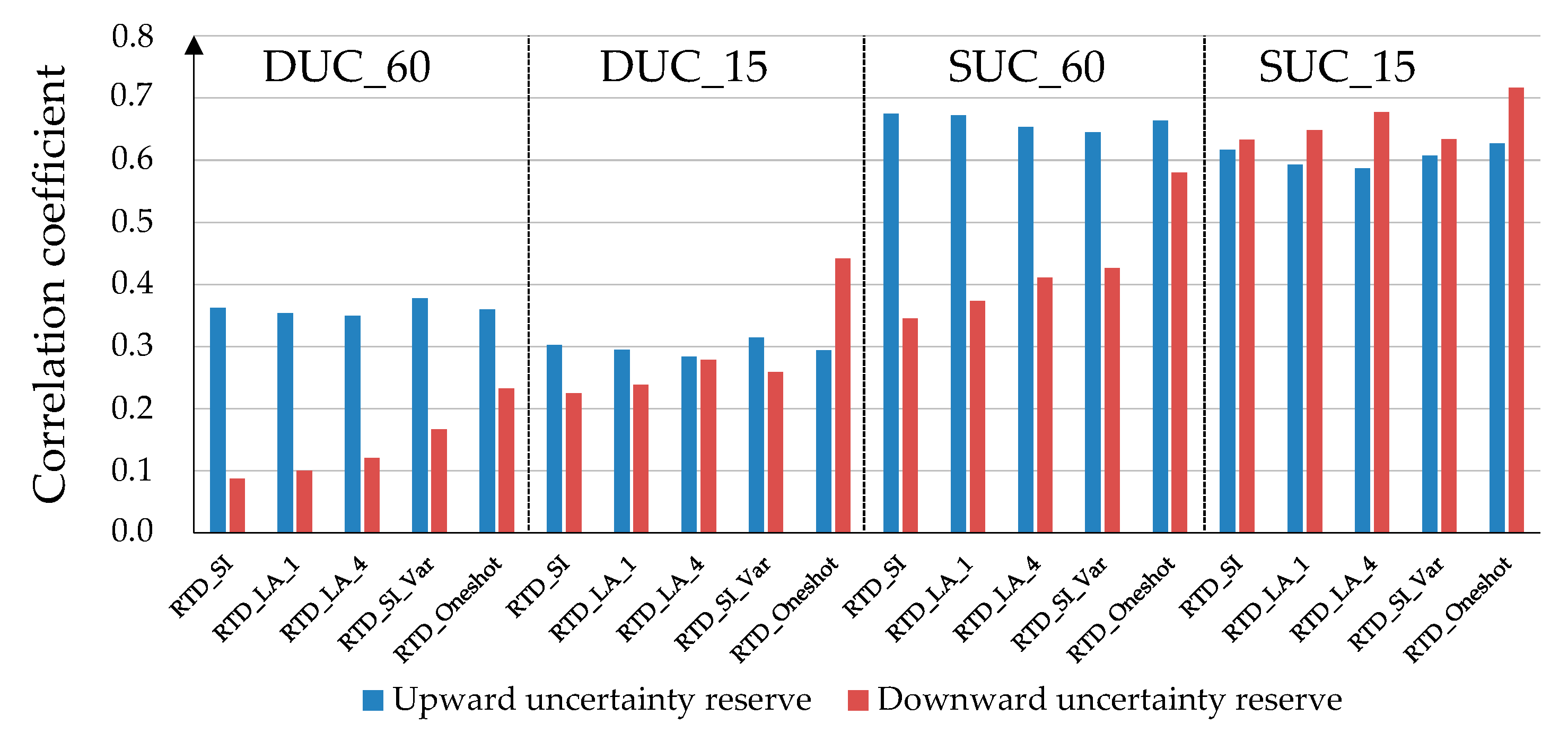
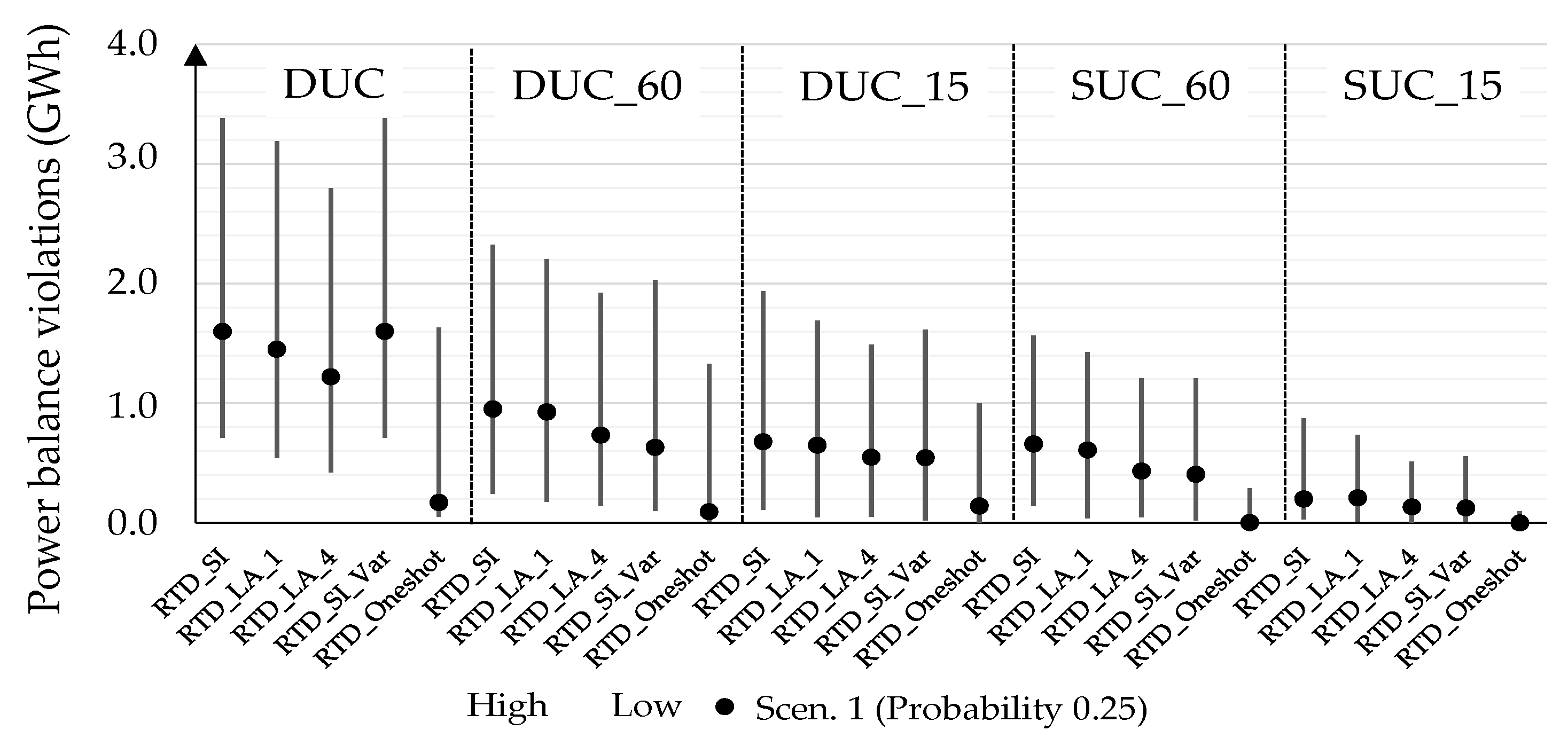
The results demonstrate the enhanced reliability achieved in RTD by applying the multi-timing scheduling concept and explicitly considering the variability reserve in day-ahead. The SUC policies tend to allocate the reserves in lower cost resources (as compared to DUC policies) considering their relative deployment cost, thus leading to cost reductions in RTD. However, SUC may occasionally provide a more ramp-constrained schedule leading to ramp shortage augmentation in RTD. Also, the correlation between the awarded uncertainty reserves in day-ahead UC and the deployed uncertainty reserves (by the awarded resources) in RTD has proven higher in the stochastic cases.

The main contributions of this paper are summarized as follows: (a) an explicit distinction is made between the uncertainty and the variability reserve, both falling into the general category of operating reserves; (b) comparable methodologies and mathematical formulations are developed for the DUC and SUC policies, based on the proposed multi-timing scheduling concept, utilizing a detailed modeling of various generating unit operating states; (c) the two-stage SUC policy incorporates the variability reserve extending previous literature, which mainly focuses on the arrangement of renewable generation uncertainty; (d) a specific proposal is made for the quantification of the uncertainty and variability reserve requirements in the DUC policy; and (e) the mathematical formulation of different real-world RTD modes is presented and utilized for evaluating the UC results, instead of simply interpreting the day-ahead scheduling outcome.

The remaining of this paper is organized as follows: Section 2 presents the problem formulation of SUC and DUC policies, as well as the structure of different RTD regimes. Section 3 and Section 4 describe the case study and the scenario generation technique, respectively, utilized for the scope of this paper. Numerical examples are provided in Section 5, whereas Section 6 concludes the paper.

2. Mathematical Problem Formulation

2.1. General Description

The aim of the day-ahead UC phase is to provide the available resources with their optimal commitment status, their hourly energy schedules, and the binding reserve awards which will serve as a tool (for the TSO) to hedge against uncertainty and inherent variability of the net load in real-time conditions. To this end, a fundamental distinction is considered between (a) the uncertainty reserve, the procurement of which is intended to address the net load forecast errors, and (b) the variability reserve, the procurement of which is intended to reduce the probability of ramp (cf. capacity) shortages and relevant price spikes in RTD. Other ancillary services such as contingency reserves, along with possible unexpected outages in RTD, are not considered in this paper to maintain focus on normal operating conditions.

In this context, the UC model (stochastic and deterministic approach) is formulated as a co-optimization problem of energy, uncertainty and variability reserves, and constitutes a Mixed Integer Linear Programming (MILP) model. External bid-costs are considered during cost minimization for the provision of uncertainty and variability reserves, to allow for the commoditization of reserves and sufficiently incentivize flexible resources to develop and provide their fast ramp capability. For simplicity, the resources correspond to conventional thermal and hydro generating units; the inclusion of other possible eligible resources such as storage, renewables and demand response in the proposed models is straightforward. Α detailed modeling of the generating unit start-up and shut-down procedures is utilized at the day-ahead UC stage, which is followed accurately in RTD.

Most notably, the concept of multi-timing scheduling is proposed and applied appropriately in the stochastic and deterministic UC policies. Multi-timing scheduling allows for the determination and optimal allocation of the uncertainty and variability reserves based on an intra-hourly (real-time) resolution, when simultaneously optimizing energy and the commitment status of the resources over longer scheduling intervals (hours). 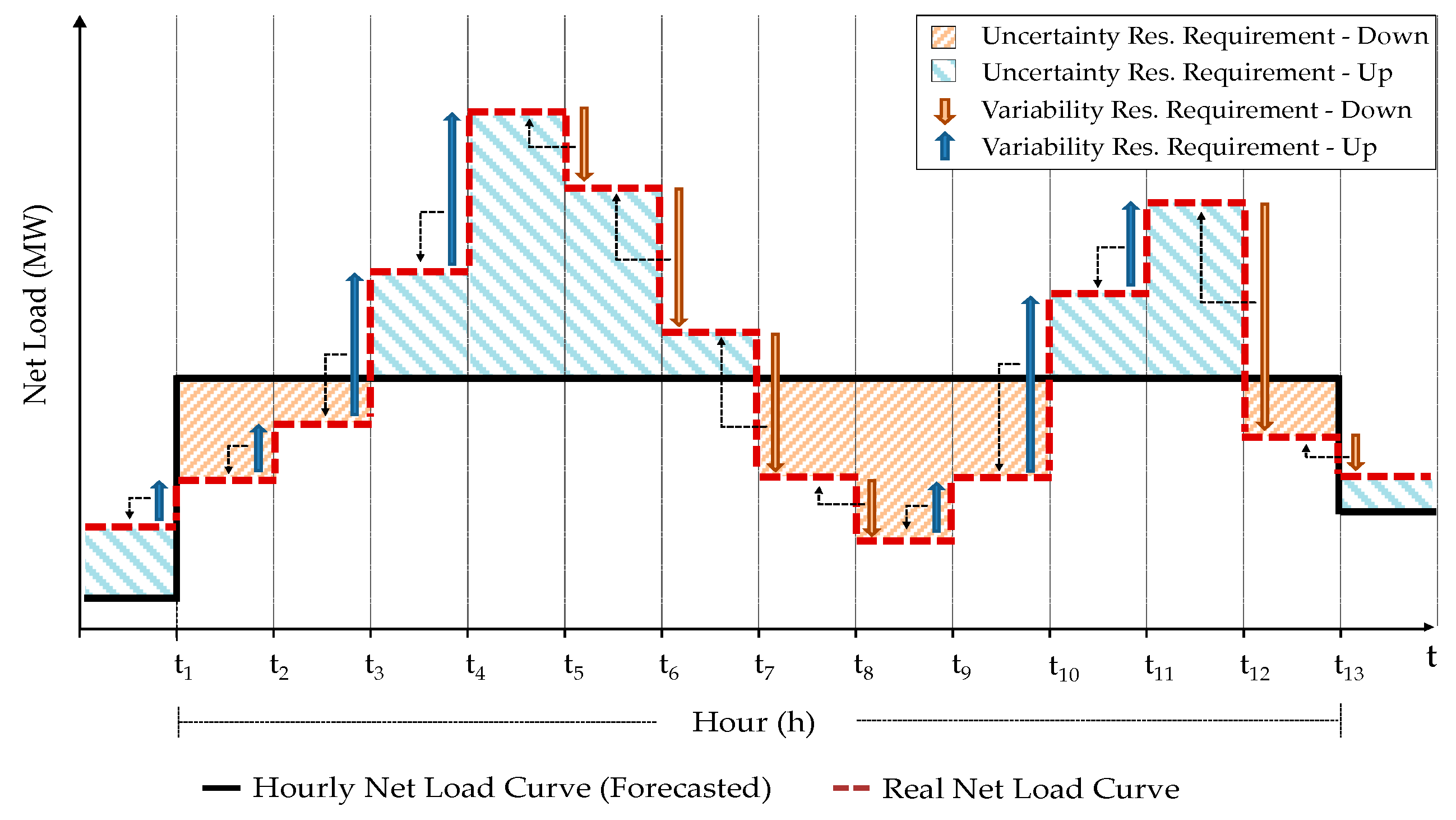Figure 1 depicts the fundamental concept of determining the system uncertainty and variability reserve requirements (either inherently in the SUC policy, or exogenously in the DUC policy) in the above context. As can be seen, the uncertainty reserve is aimed to cover the net load forecast errors, namely the possible mismatches between the hourly (h) net load level forecasted day-ahead and the net load realized in each instance (t) of RTD, while the variability reserve is aimed to cover the net load variations between successive intervals (t) in RTD, with each variation being assigned as a respective requirement to the preceding real-time interval.

We thereby maintain the legitimate simplicity of the hourly commitment and scheduling solutions during the day-ahead stage. However, the utilization of real-time information and the coordination with the time resolution of RTD when procuring the respective reserves (a) brings more accuracy and efficiency on the system scheduled flexibility, by securing a dedicated capacity and ramping headroom per each specific real-time interval; (b) enhances incentives for the provision of fast (real-time) ramp capability at the scheduling stage, and thereof; (c) optimally arranges the increased net load variations in RTD associated with high penetration levels of renewable generation.

2.2. Stochastic Unit Commitment (SUC)

The structure of the SUC model is divided into two stages (two-stage stochastic programming). The first stage describes the day-ahead scheduling decisions (optimal commitment, hourly energy schedules, uncertainty and variability reserve awards), while the second considers various possible realizations of the power system operation through a set of net load scenarios, in order to determine the optimal reserve awards of the first stage in an accurate and economic (in terms of actual deployment) manner. Since the second stage models real-time operation, and in order to attain advanced flexibility features in the scheduling results, the utilization of finer time resolution is proposed at this stage, coordinated with the time-step of the RTD function, which addresses both the increased intra-hourly forecast errors (uncertainty) and the steep intra-hourly system ramping requirements (variability) that may occur during RTD.

2.2.1. Objective Function

The TSO total cost (1) to be minimized over the scheduling period consists of (in order of appearance of the various terms): (a) the resources’ commitment (start-up and shut-down) costs; (b) the hourly procurement (as-bid) costs of energy; (c) uncertainty and (d) variability reserves at the first stage, as well as; (e) the intra-hourly deployment cost of the uncertainty reserve, along with the load shedding and wind spillage cost, at the second stage, weighted by the respective probability of each net load scenario:

$$\begin{array}{l}\mathrm{Min} F_{SUC}={\displaystyle \sum _{i\in I}{\displaystyle \sum _{h\in \mathcal{H}}\left(S{U}_i\cdot y_{ih}+S{D}_i\cdot z_{ih}\right)}}+{\displaystyle \sum _{i\in I}{\displaystyle \sum _{h\in \mathcal{H}}{\displaystyle \sum _{k\in \mathcal{K}}\left(q_{ihk}\cdot C_{ihk}^{en}\right)}}}+{\displaystyle \sum _{i\in I}{\displaystyle \sum _{h\in \mathcal{H}}\left(r_{ih}^{un{c}^{up}}\cdot C_{ih}^{un{c}^{up}}+r_{ih}^{un{c}^{dn}}\cdot C_{ih}^{un{c}^{dn}}\right)}}\\ +{\displaystyle \sum _{i\in I}{\displaystyle \sum _{h\in \mathcal{H}}\left(r_{ih}^{va{r}^{up}}\cdot C_{ih}^{{\mathit{var}}^{up}}+r_{ih}^{va{r}^{dn}}\cdot C_{ih}^{{\mathit{var}}^{dn}}\right)}}+\frac{{\Delta }^{RTD}}{{\Delta }^{UC}}\cdot {\displaystyle \sum _{s\in S}{\pi }_s\left\{{\displaystyle \sum _{i\in I}{\displaystyle \sum _{t\in \mathcal{T}}{\displaystyle \sum _{k\in \mathcal{K}}\left(r_{itsk}^{unc}\cdot C_{itk}^{en}\right)}}}+{\displaystyle \sum _{t\in \mathcal{T}}\left(l_{ts}^{Sh}\cdot C_t^{Sh}+w_{ts}^{Sp}\cdot C_t^{Sp}\right)}\right\}}\end{array}$$

(1)

The term $\frac{{\Delta }^{RTD}}{{\Delta }^{UC}}$ is used to account for the intra-hourly resolution considered at the second stage of the SUC model, for example it is equal to ¼ in case a quarterly resolution is applied.

2.2.2. Day-Ahead Market Constraints (1st Stage)

The constraints utilized in the first stage of the SUC model are scenario independent and apply to each hourly interval h of the daily scheduling horizon. The following set (2)–(6) models the generating unit operating states of synchronization (2), stepwise soak (3) based on hourly energy soak steps (4) as pre-defined by the producer, and stepwise desynchronization (5) following a linear decrease rate (6). For an analytical description of these constraints the reader is referred to [56].

$$\begin{array}{cc}{u}_{ih}^{syn}={\displaystyle \sum _{\tau =h-T_i^{syn}+1}^h{y}_{i\tau }}& \forall i\in I,h\in \mathcal{H}\end{array}$$

(2)

$$\begin{array}{cc}{u}_{ih}^{soak}={\displaystyle \sum _{\tau =h-T_i^{syn}-T_i^{soak}+1}^{h-T_i^{syn}}{y}_{i\tau }}& \forall i\in I,h\in \mathcal{H}\end{array}$$

(3)

$$\begin{array}{cc}{p}_{ih}^{soak}={\displaystyle \sum _{f=1}^{T_i^{soak}}{P}_{if}^{soak}\cdot y_{i,h-(T_i^{syn}+f-1)}}& \forall i\in I, h\in \mathcal{H}\end{array}$$

(4)

$$\begin{array}{cc}{u}_{ih}^{des}={\displaystyle \sum _{\tau =h+1}^{h+T_i^{des}-1}{z}_{i\tau }}& \forall i\in I,h\in \mathcal{H}\end{array}$$

(5)

$$\begin{array}{cc}{p}_{ih}^{des}={\displaystyle \sum _{\tau =h}^{h+T_i^{des}-1}{z}_{i\tau }}\cdot \left(\tau -h\right)\cdot \frac{P_i^{\min }}{T_i^{des}}& \forall i\in I,h\in \mathcal{H}\end{array}$$

(6)

Inequalities (7) and (8) denote the minimum up and down time constraints of the generating units, respectively,

$$\begin{array}{cc}{\displaystyle \sum _{\tau =h-U{T}_i+1}^h{y}_{i\tau }\le u_{ih}}& \forall i\in I,h\in \mathcal{H}\end{array}$$

(7)

$$\begin{array}{cc}{\displaystyle \sum _{\tau =h-D{T}_i+1}^h{z}_{i\tau }\le 1-u_{ih}}& \forall i\in I,h\in \mathcal{H}\end{array}$$

(8)

while (9)–(13) describe the logical relations of the commitment binary variables.

$$\begin{array}{cc}{u}_{ih}=u_{ih}^{syn}+u_{ih}^{soak}+u_{ih}^{disp}+u_{ih}^{des}& \forall i\in I,h\in \mathcal{H}\end{array}$$

(9)

$$\begin{array}{cc}{y}_{ih}-z_{ih}=u_{ih}-u_{i\left(h-1\right)}& \forall i\in I,h\in \mathcal{H}\end{array}$$

(10)

$$\begin{array}{cc}{y}_{ih}+z_{ih}\le 1& \forall i\in I,h\in \mathcal{H}\end{array}$$

(11)

$$\begin{array}{cc}{u}_{ih}\ge y_{ih}& \forall i\in I,h\in \mathcal{H}\end{array}$$

(12)

$$\begin{array}{cc}{u}_{ih}\ge z_{i(h+1)}& \forall i\in I,h\in \mathcal{H}\end{array}$$

(13)

In (14) and (15), the hourly day-ahead energy schedule of each unit ($p_{ih}$) is coordinated with the respective upward and downward uncertainty reserve, within the unit technical limits in every operating state (i.e., synchronization, soak, normal dispatch or desynchronization). Apparently, the uncertainty reserve can be allocated only during the phase of normal dispatch (i.e., unit operation between its technical minimum and maximum limit). The last term in the right-hand side of (14) is used to equalize the output of a unit with its technical minimum production at the hour prior to the desynchronization process, and is omitted for units with desynchronization time less than one hour.

$$\begin{array}{cc}{p}_{ih}+r_{ih}^{un{c}^{up}}\le 0\cdot u_{ih}^{syn}+p_{ih}^{soak}+p_{ih}^{des}+P_i^{\max }\cdot u_{ih}^{disp}+\left(P_i^{\min }-P_i^{\max }\right)\cdot z_{i(h+T_i^{des})}& \forall i\in I,h\in \mathcal{H}\end{array}$$

(14)

$$\begin{array}{cc}{p}_{ih}-r_{ih}^{un{c}^{dn}}\ge 0\cdot u_{ih}^{syn}+p_{ih}^{soak}+p_{ih}^{des}+P_i^{\min }\cdot u_{ih}^{disp}& \forall i\in I,h\in \mathcal{H}\end{array}$$

(15)

In (16), the hourly energy schedule of a unit is derived from the cleared quantities of all steps k of the associated unit offer, while in (17) the cleared quantity of each step is limited by the offered size of the step.

$$\begin{array}{cc}{p}_{ih}={\displaystyle \sum _{k\in \mathcal{K}}{q}_{ihk}}& \forall i\in I,h\in \mathcal{H}\end{array}$$

(16)

$$\begin{array}{cc}0\le q_{ihk}\le Q_{ihk}^{\max }& \forall i\in I,h\in \mathcal{H},k\in \mathcal{K}\end{array}$$

(17)

Constraints (18) and (19) enforce the ramp rate limits on the unit power output between consecutive hourly (${\Delta }^{UC}$) time intervals. The last terms in the right-hand side of (18) and (19) relax the ramp limits during the synchronization, soak and desynchronization phases.

$$\begin{array}{cc}{p}_{ih}-p_{i\left(h-1\right)}\le {\Delta }^{UC}\cdot R{U}_i\cdot u_{ih}^{disp}+B\cdot \left(u_{ih}^{syn}+u_{ih}^{soak}\right)& \forall i\in I,h\in \mathcal{H}\end{array}$$

(18)

$$\begin{array}{cc}{p}_{i\left(h-1\right)}-p_{ih}\le {\Delta }^{UC}\cdot R{D}_i\cdot u_{ih}^{disp}+B\cdot \left(z_{ih}+u_{ih}^{des}\right)& \forall i\in I,h\in \mathcal{H}\end{array}$$

(19)

Finally, in power balance Equation (20) the energy procured from all conventional generating units covers the hourly net load forecasted at the day-ahead stage.

$$\begin{array}{cc}{\displaystyle \sum _{i\in I}{p}_{ih}}=L_h-W_h& \forall h\in \mathcal{H}\end{array}$$

(20)

Within the scope of this paper, renewable generation is represented by wind production, which is assumed to be a regulated (non-competitive) activity given dispatch priority, as is currently the case for existing wind plants in most energy systems around the world. Thus, wind producers do not submit offers in the market and the forecasted wind generation $W_h$ is considered as negative demand in (20). However, there is the possibility for wind generation to be spilled at extreme scenarios considered in the second stage of the SUC model (see power balance Equation (31)).

2.2.3. Real-Time Operation Constraints (2nd Stage)

The multi-timing scheduling concept requires that the second stage of the SUC model (a) considers the realization of a number of possible net load scenarios s based on the finer (intra-hourly) time resolution t applying in RTD; (b) calculates the optimal uncertainty and variability reserve quantities that are actually deployed in each real-time interval t and scenario s; and thereby (c) determines the respective hourly uncertainty and variability reserves to be allocated to the various resources at the day-ahead (first) stage.

More specifically, in equality (21), the upward (downward) uncertainty reserve deployed is essentially the incremental (decremental) energy procured by unit i in scenario s and real-time interval t, over the unit day-ahead schedule ($p_{ih}$) for the corresponding hour h. The resulting real-time schedule $p_{its}$ is placed within the unit technical limits in every operating state, in constraints (22) and (23). Note the special handling for the coordination of the real-time (t) variables with the respective hourly (h) variables in the formulation of (21)–(23) (i.e., these constraints apply $\forall h\in \mathcal{H}$ and simultaneously $\forall t\in {\mathcal{T}}_h$).

$$\begin{array}{cc}{p}_{its}=p_{ih}+r_{its}^{un{c}^{up}}-r_{its}^{un{c}^{dn}}& \forall i\in I, h\in \mathcal{H},t\in {\mathcal{T}}_h, s\in S\end{array}$$

(21)

$$\begin{array}{cc}{p}_{its}\le 0\cdot u_{ih}^{syn}+p_{ih}^{soak}+p_{ih}^{des}+P_i^{\max }\cdot u_{ih}^{disp}& \forall i\in I, h\in \mathcal{H},t\in {\mathcal{T}}_h, s\in S\end{array}$$

(22)

$$\begin{array}{cc}{p}_{its}\ge 0\cdot u_{ih}^{syn}+p_{ih}^{soak}+p_{ih}^{des}+P_i^{\min }\cdot u_{ih}^{disp}& \forall i\in I,h\in \mathcal{H},t\in {\mathcal{T}}_h, s\in S\end{array}$$

(23)

Note also, that by summing each side of (21) for all units i, the term in the left-hand side essentially provides the real-time net load for scenario s and time interval t, the first term of the right-hand side provides the hourly net load forecasted at the day-ahead stage, while the two latter terms provide the respective system uncertainty reserve requirements in each direction, respectively, for the given scenario s and real-time interval t. That is, the uncertainty reserve requirements per scenario s are determined as the difference between the real-time net load and the respective hourly net load forecasted at the day-ahead stage, in line with the relevant description provided in Figure 1.

Accordingly, in (24), the variability reserve deployed by unit i in each real-time interval t − 1 is essentially the variation of the unit’s power output $p_{its}$ between the successive intervals t − 1 and t, for a given scenario s. In case of positive variations, upward variability reserve is deployed, and vice versa. The variability reserve deployed is in turn limited by the unit ramp capability over the length of the real-time interval (${\Delta }^{RTD}$) in (25) and (26) for the upward and downward direction, respectively.

$$\begin{array}{cc}{p}_{its}-p_{i\left(t-1\right)s}=r_{i\left(t-1\right)s}^{va{r}^{up}}-r_{i\left(t-1\right)s}^{va{r}^{dn}}& \forall i\in I,t\in \mathcal{T}, s\in S\end{array}$$

(24)

$$\begin{array}{cc}0\le r_{its}^{va{r}^{up}}\le {\Delta }^{RTD}\cdot R{U}_i& \forall i\in I, t\in \mathcal{T}, s\in S\end{array}$$

(25)

$$\begin{array}{cc}0\le r_{its}^{va{r}^{dn}}\le {\Delta }^{RTD}\cdot R{D}_i& \forall i\in I, t\in \mathcal{T}, s\in S\end{array}$$

(26)

Note again, that by summing each side of (24) for all units i, the left-hand side provides the net load variations between successive real-time intervals t in each scenario s, while the right-hand side provides the corresponding system variability reserve requirements; each net load variation (i.e., between t − 1 and t) is assigned as a respective requirement to the preceding real-time interval (i.e., t − 1), in line with the relevant description provided in Figure 1.

In order for the hourly uncertainty and variability reserves of the first stage to be calculated over all (independent of the) scenarios considered at the second stage, the linking constraints (27) and (28) are applied. In (27), the largest uncertainty reserve deployed by unit i among all real-time intervals t belonging to hour h, and among all scenarios s of the second stage, defines the respective hourly uncertainty reserve award of that unit for the given hour h. A similar approach is also applicable for the variability reserve in (28). In this case, the hourly (first-stage) variability reserve award of a unit (right-hand side of (28)) is defined based on the largest algebraic summation of the variability reserves deployed by that unit within the given hour h, among all scenarios s of the second stage. In this context, the unit is remunerated through the hourly variability reserve award for all real-time variations of its power output expected to realize within said hour in RTD (since the TSO has hedged its position against all real-time variations of the net load, respectively), acquiring stronger incentives to provide its ramp capability in real-time conditions.

$$\begin{array}{cc}{r}_{its}^m\le r_{ih}^m& \forall i\in I, h\in \mathcal{H}, t\in {\mathcal{T}}_h, s\in S, m\in \left\{un{c}^{up},un{c}^{dn}\right\}\end{array}$$

(27)

$$\begin{array}{cc}{\displaystyle \sum _{t\in {\mathcal{T}}_h}{r}_{its}^m}\le r_{ih}^m& \forall i\in I,h\in \mathcal{H}, s\in S, m\in \left\{va{r}^{up},va{r}^{dn}\right\}\end{array}$$

(28)

With regard to the additional cost of deployment of the uncertainty reserve at the second stage, the right-hand side of (29) determines the quantity deployed (positive if upward reserve is deployed, and vice versa) per step k of the associated energy offer, and the relevant cost of deployment (energy cost) is considered in the last term of the objective function (1). Note that a similar deployment (energy) cost for the variability reserve shall not explicitly be defined in (1), put it differently, the deployment of the variability reserve refers to the variations of the unit output between consecutive real-time intervals and not to the actual energy level in each specific interval. Inequalities (30) calculate the remaining margins (in both directions) for uncertainty reserve deployment per step k of the unit energy offer, as compared to the energy procured by that unit at the first stage ($q_{ihk}$).

$$\begin{array}{cc}{r}_{its}^{un{c}^{up}}-r_{its}^{un{c}^{dn}}={\displaystyle \sum _{k\in \mathcal{K}}{r}_{itsk}^{unc}}& \forall i\in I,t\in \mathcal{T}, s\in S\end{array}$$

(29)

$$\begin{array}{cc}-q_{ihk}\le r_{itsk}^{unc}\le Q_{ihk}^{\max }-q_{ihk}& \forall i\in I,h\in \mathcal{H}, t\in {\mathcal{T}}_h, s\in S, k\in \mathcal{K}\end{array}$$

(30)

Finally, (31) enforces the power balance equation at the second stage of the SUC model, where the possibility for load shedding and wind spillage in extreme scenarios is also considered.

$$\begin{array}{cc}{\displaystyle \sum _{i\in I}{p}_{its}}=\left(L_{ts}-l_{ts}^{Sh}\right)-\left(W_{ts}-w_{ts}^{Sp}\right)& \forall t\in \mathcal{T},s\in S\end{array}$$

(31)

2.3. Deterministic Unit Commitment (DUC)

In contrast to the SUC model, which determines the day-ahead uncertainty and variability reserve awards inherently (i.e., through the consideration of different possible net load scenarios at the second stage and the linking constraints), the DUC model calculates the optimal reserve allocation through pre-determined reserve requirements defined rather exogenously. That is, the DUC model is similar to the one presented in Section 2.2, but with the following exceptions: (a) constraints (21)–(31) pertaining to the second stage of the SUC model are replaced by (32), (33) and (38)–(42) presented hereinafter; and (b) the last term of the objective function (1) (regarding the deployment cost of the uncertainty reserve) is apparently omitted. Then, the DUC problem formulation is as follows:

Min F_DUC, subject to (2)–(20), (32), (33), (38)–(42)

Constraints (32) and (33) ensure that the total contribution in each type of reserve meets the associated system requirements:

$$\begin{array}{cc}{\displaystyle \sum _{i\in I}{r}_{ih}^m}\ge Re{q}_h^m& \forall h\in \mathcal{H}, m\in \left\{un{c}^{up},un{c}^{dn}\right\}\end{array}$$

(32)

$$\begin{array}{cc}{\displaystyle \sum _{i\in I}{r}_{it}^m}\ge Re{q}_t^m& \forall t\in \mathcal{T}, m\in \left\{va{r}^{up},va{r}^{dn}\right\}\end{array}$$

(33)

The multi-timing scheduling concept in the DUC policy requires that the reserve requirements are determined as per the following formulas (34)–(37) utilizing real-time information for both types of reserves (uncertainty and variability), according to the relevant description of Figure 1. In (34)/(35), the largest difference between the hourly net load forecasted at the day-ahead stage and the real-time net load (considering all corresponding intervals t and scenarios s) determines the upward/downward uncertainty reserve requirement for hour h. Accordingly, in (36)/(37), the largest variation of the net load between successive real-time intervals t and t + 1 (considering all scenarios s) determines the upward/downward variability reserve requirement for real-time interval t.

$$\begin{array}{cc}Re{q}_h^{un{c}^{up}}=\underset{s\in S, t\in {\mathcal{T}}_h}{\mathrm{Max}}\left[0,\left(L_{ts}-W_{ts}\right)-\left(L_h-W_h\right)\right]& \forall h\in \mathcal{H}\end{array}$$

(34)

$$\begin{array}{cc}Re{q}_h^{un{c}^{dn}}=\underset{s\in S, t\in {\mathcal{T}}_h}{\mathrm{Max}}\left[0,\left(L_h-W_h\right)-\left(L_{ts}-W_{ts}\right)\right]& \forall h\in \mathcal{H}\end{array}$$

(35)

$$\begin{array}{cc}Re{q}_t^{va{r}^{up}}=\underset{s\in S}{\mathrm{Max}}\left[0,\left(L_{\left(t+1\right)s}-W_{\left(t+1\right)s}\right)-\left(L_{ts}-W_{ts}\right)\right]& \forall t\in \mathcal{T}\end{array}$$

(36)

$$\begin{array}{cc}Re{q}_t^{va{r}^{dn}}=\underset{s\in S}{\mathrm{Max}}\left[0,\left(L_{ts}-W_{ts}\right)-\left(L_{\left(t+1\right)s}-W_{\left(t+1\right)s}\right)\right]& \forall t\in \mathcal{T}\end{array}$$

(37)

Note that the load and wind power dataset utilized for the quantification of the deterministic reserves essentially comprises the same real-time scenarios s also considered in the stochastic approach (second stage), for homogeneity purposes. Nevertheless, the same methodology (34)–(37) can also be implemented on the initial (historic) load and wind power dataset utilized for the creation of scenarios (Section 4), replacing the Max criterion by a certain percentile (e.g., 99%) of the respective error/variation probability distributions. In any case, the herein approach provides an accurate method of quantifying the deterministic reserves, which is comparable to the respective SUC functionality at the second stage, as compared to utilizing trial-based values [41] or simplified/heuristic approaches for determining the reserve requirements (e.g., a constant requirement representing a certain fraction of the peak load [43], or the 3 + 5 rule [12]), or not imposing reserve requirements in the DUC policy at all.

Moreover, the variability reserve requirements are explicitly determined in (36) and (37) per real-time interval t, and allocated to the eligible resources based on their real-time ramp capability through the following constraints (38) and (39). These constraints are similar to (25) and (26) of the SUC model, and are used to allocate the variability reserve to faster resources in case of increased intra-hourly net load variations expected in RTD:

$$\begin{array}{cc}{r}_{it}^{va{r}^{up}}\le {\Delta }^{RTD}\cdot R{U}_i\cdot u_{ih}^{disp}& \forall i\in I, h\in \mathcal{H},t\in {\mathcal{T}}_h\end{array}$$

(38)

$$\begin{array}{cc}{r}_{it}^{va{r}^{dn}}\le {\Delta }^{RTD}\cdot R{D}_i\cdot u_{ih}^{disp}& \forall i\in I, h\in \mathcal{H},t\in {\mathcal{T}}_h\end{array}$$

(39)

The respective hourly variability reserve award of each unit is then calculated in (40) (similarly to constraint (28) of the SUC model):

$$\begin{array}{cc}{\displaystyle \sum _{t\in {\mathcal{T}}_h}{r}_{it}^m}=r_{ih}^m& \forall i\in I,h\in \mathcal{H}, m\in \left\{va{r}^{up},va{r}^{dn}\right\}\end{array}$$

(40)

Finally, the following constraints (41) and (42) are additionally enforced in the DUC model, in order to delimit the upward and downward variability reserve award of a unit in the range $P_i^{\max }-P_i^{\min }$.

$$\begin{array}{cc}{p}_{ih}+r_{ih}^{va{r}^{up}}-r_{ih}^{un{c}^{dn}}\le 0\cdot u_{ih}^{syn}+p_{ih}^{soak}+p_{ih}^{des}+P_i^{\max }\cdot u_{ih}^{disp}& \forall i\in I,h\in \mathcal{H}\end{array}$$

(41)

$$\begin{array}{cc}{p}_{ih}-r_{ih}^{va{r}^{dn}}+r_{ih}^{un{c}^{up}}\ge 0\cdot u_{ih}^{syn}+p_{ih}^{soak}+p_{ih}^{des}+P_i^{\min }\cdot u_{ih}^{disp}& \forall i\in I,h\in \mathcal{H}\end{array}$$

(42)

The utilization of the downward uncertainty reserve in a counteractive manner to the upward variability reserve in the left-hand side of (41) is motivated by the following possible outcome noticed in the SUC model respectively: a unit is scheduled at its maximum level in a given hour at the first stage, in parallel receives a downward uncertainty reserve award for that hour (obtained due to a low scenario at the second stage), while at the same time the unit receives an upward variability award (i.e., the unit was ramping up in said low scenario at the second stage). That is, in case the low scenario actually materializes in real time, the unit is expected to be producing at a lower level, thereby also being able to ramp-up in the given hour. A respective concept also applies to constraint (42) for the downward direction.

2.4. Real-Time Dispatch (RTD)

The RTD function is utilized in this paper in order to evaluate the scheduling results of any UC policy (stochastic and deterministic approach). Elsewhere, the literature often determines the expected cost in real-time operation directly from the solution of the SUC model (cost of each scenario at the second stage multiplied by the respective probability of occurrence), e.g., [46], or by implementing additional Monte Carlo simulations for a number of net load realizations, each one solved one-shot for the whole scheduling horizon based on the commitments produced by the UC process, e.g., [41]. In order to replicate more accurately the RTD applications in real world and reveal some implications relative to the nature of the RTD regime used, the deterministic RTD, herein, is simulated as a rolling dispatch procedure (i.e., solved sequentially for each real-time interval), with none or limited [57] look-ahead capability, or with the use of the variability reserve [32,33,34,35] determined by the UC application. The baseline RTD mathematical formulation is the following:

$$\mathrm{Min}{F}_{RTD}=\frac{{\Delta }^{RTD}}{{\Delta }^{UC}}\cdot \left\{{\displaystyle \sum _{i\in I}{\displaystyle \sum _{t\in {\mathcal{T}}^{RTD}}{\displaystyle \sum _{k\in \mathcal{K}}\left(q_{itk}\cdot C_{itk}^{en}\right)}}}+{\displaystyle \sum _{t\in {\mathcal{T}}^{RTD}}\left(l_t^{Sh}\cdot C_t^{Sh}+w_t^{Sp}\cdot C_t^{Sp}\right)}+{\displaystyle \sum _{i\in I}{\displaystyle \sum _{t\in {\mathcal{T}}^{RTD}}\left(de{f}_{it}^{va{r}^{up}}+de{f}_{it}^{va{r}^{dn}}\right)\cdot C_t^{def}}}\right\}$$

(43)

$$\begin{array}{cc}{p}_{it}={\overline{p}}_{ih}+r_{it}^{un{c}^{up}}-r_{it}^{un{c}^{dn}}& \forall i\in I, t\in {\mathcal{T}}_h^{RTD}\end{array}$$

(44)

$$\begin{array}{cc}{p}_{it}\le 0\cdot {\overline{u}}_{ih}^{syn}+{\overline{p}}_{ih}^{soak}+{\overline{p}}_{ih}^{des}+P_i^{\max }\cdot {\overline{u}}_{ih}^{disp}& \forall i\in I, t\in {\mathcal{T}}_h^{RTD}\end{array}$$

(45)

$$\begin{array}{cc}{p}_{it}\ge 0\cdot {\overline{u}}_{ih}^{syn}+{\overline{p}}_{ih}^{soak}+{\overline{p}}_{ih}^{des}+P_i^{\min }\cdot {\overline{u}}_{ih}^{disp}& \forall i\in I,t\in {\mathcal{T}}_h^{RTD}\end{array}$$

(46)

$$\begin{array}{cc}{p}_{it}-p_{i\left(t-1\right)}\le {\Delta }^{RTD}\cdot R{U}_i\cdot {\overline{u}}_{ih}^{disp}+B\cdot \left({\overline{u}}_{ih}^{syn}+{\overline{u}}_{ih}^{soak}\right)& \forall i\in I, t\in {\mathcal{T}}_h^{RTD}\end{array}$$

(47)

$$\begin{array}{cc}{p}_{i\left(t-1\right)}-p_{it}\le {\Delta }^{RTD}\cdot R{D}_i\cdot {\overline{u}}_{ih}^{disp}+B\cdot \left({\overline{u}}_{ih}^{des}+{\overline{z}}_{ih}\right)& \forall i\in I, t\in {\mathcal{T}}_h^{RTD}\end{array}$$

(48)

$$\begin{array}{cc}{p}_{it}={\displaystyle \sum _{k\in \mathcal{K}}{q}_{itk}}& \forall i\in I,t\in {\mathcal{T}}^{RTD}\end{array}$$

(49)

$$\begin{array}{cc}0\le q_{itk}\le Q_{itk}^{\max }& \forall i\in I, t\in {\mathcal{T}}^{RTD},k\in \mathcal{K}\end{array}$$

(50)

$$\begin{array}{cc}{\displaystyle \sum _{i\in I}{p}_{it}}=\left(L_t-l_t^{Sh}\right)-\left(W_t-w_t^{Sp}\right)& \forall t\in {\mathcal{T}}^{RTD}\end{array}$$

(51)

$$\begin{array}{cc}{p}_{it}+r_{it}^{va{r}^{up}}\le 0\cdot {\overline{u}}_{ih}^{syn}+{\overline{p}}_{ih}^{soak}+{\overline{p}}_{ih}^{des}+P_i^{\max }\cdot {\overline{u}}_{ih}^{disp}& \forall i\in I, t\in {\mathcal{T}}_h^{RTD}\end{array}$$

(52)

$$\begin{array}{cc}{p}_{it}-r_{it}^{va{r}^{dn}}\ge 0\cdot {\overline{u}}_{ih}^{syn}+{\overline{p}}_{ih}^{soak}+{\overline{p}}_{ih}^{des}+P_i^{\min }\cdot {\overline{u}}_{ih}^{disp}& \forall i\in I,t\in {\mathcal{T}}_h^{RTD}\end{array}$$

(53)

$$\begin{array}{cc}{r}_{it}^{va{r}^{up}}+de{f}_{it}^{va{r}^{up}}\ge {\overline{r}}_{it}^{va{r}^{up}}& \forall i\in I, t\in {\mathcal{T}}^{RTD}\end{array}$$

(54)

$$\begin{array}{cc}{r}_{it}^{va{r}^{dn}}+de{f}_{it}^{va{r}^{dn}}\ge {\overline{r}}_{it}^{va{r}^{dn}}& \forall i\in I, t\in {\mathcal{T}}^{RTD}\end{array}$$

(55)

For each subsequent RTD execution, the energy, load shedding and wind spillage costs are minimized in the objective function (43) over the given dispatch horizon ${\mathcal{T}}^{RTD}$. In the constraints following objective (43), the value of all variables denoted with an upper dash, like the commitment status, has already been determined by the UC solution and is not re-optimized in RTD. In that respect, (44) describes the actual deployment of the uncertainty reserve by each unit in RTD as compared to its hourly day-ahead energy schedule, (45) and (46) impose the unit power output limits in every operating state, (47) and (48) enforce the ramping constraints, (49) and (50) determine the unit output based on the maximum offered quantity per step of the associated energy offer, while (51) describes the power balance equation. The latter constraints (52)–(55) are used only in the RTD mode RTD_SI_Var (explained below) to consider the variability reserve as an alternative way of “looking ahead” in RTD.

In this context, five RTD modes are used to evaluate the UC outcome, as follows:

• RTD_SI (model (43)–(51)): RTD economically dispatches the committed resources for each subsequent real-time interval without future expectation of the net load (single-interval or blind mode); set ${\mathcal{T}}^{RTD}$ essentially comprises only one element, i.e., the current interval.
• RTD_LA_1 (model (43)–(51)): RTD economically dispatches the committed resources for each subsequent real-time interval, while also looking ahead to the following interval. In each clearance, the dispatch solution for the first interval is binding, while the solution for the look-ahead interval is only advisory.
• RTD_LA_4 (model (43)–(51)): Similar to RTD_LA_1, however the look-ahead horizon is extended to four real-time intervals.
• RTD_SI_Var (model (43), (44), (47)–(55)): Similarly to RTD_SI, a single-interval dispatch is implemented, however the variability reserve awards determined by the UC application are used in (52)–(55) to keep the dispatch schedule of the eligible resources “away” from their technical maximum (52) (or minimum (53)) limit in previous RTD intervals, so as they can provide their upward (or downward) ramping headroom in future intervals, when mostly needed. The variability reserve product has been introduced along with variability reserve requirements in RTD by the CAISO [32,34] and the MISO [33,35] in a similar way. The new product, commonly called “flexiramp”, is intended to establish sufficient ramping margins between consecutive time intervals of the optimization process and thereby reduce the frequency of temporary ramp shortages in the real-time market, while also producing a sufficient revenue for economic resources being held back in previous RTD intervals in order to provide their ramping capacity towards future intervals. Note that when a similar situation takes place by implementing multi-interval (look-ahead) RTD (instead of utilizing the variability reserve), for example when the generation of an economic unit is held back from its maximum limit in the current real-time interval due to the need to provide upward ramping towards the following (look-ahead) interval, the resource suffers from a lost revenue in the first interval which is never settled upon, thereby receiving weaker incentives to actually provide the required flexibility [37]. It is that price-incentivizing structure that brings an increasing interest to the use of the flexiramp product. The only difference, herein, is that the variability reserve requirements are not re-allocated in RTD. Instead, the variability reserve variable of each unit in the left-hand side of (52) and (53) is determined by the respective day-ahead UC award through (54) and (55). We thereby examine the pure impact of the UC pre-determined variability reserve quantities on the outcome of RTD. The only case that the variability reserve quantity of a unit in a given interval is not fulfilled by the respective UC award is when such quantity is actually dispatched in order to avoid a power balance violation in the current interval, rather than being secured to meet the expected variability in future intervals. This is achieved in RTD_SI_Var by imposing a lower penalty price on variability reserve deficits incurred in (54) and (55) (see the last term of objective (43)), as compared to the penalty prices imposed for load shedding and wind spillage.
• RTD_Oneshot (model (43)–(51)): RTD economically dispatches the committed resources in an one-shot solution for the whole daily scheduling horizon, for comparison purposes; set ${\mathcal{T}}^{RTD}$ essentially comprises all real-time intervals of the daily horizon.

3. Case Study

The proposed UC policies are tested using a modified version of the Greek interconnected power system for the daily scheduling period of 31 March 2014. A summary of the conventional generating unit techno-economic characteristics is presented on

Table 1. Summary of the generation techno-economic data for the modified Greek power system.

Unit Categ.	Num	${\mathit{P}}_{\mathit{i}}^{\mathbf{max}}$ (MW)	${\mathit{P}}_{\mathit{i}}^{\mathbf{min}}$ (MW)	$\mathit{R}{\mathit{U}}_{\mathit{i}}\mathbf{/}\mathit{R}{\mathit{D}}_{\mathit{i}}$ (MW/min)	$\mathit{U}{\mathit{T}}_{\mathit{i}}$ (h)	$\mathit{D}{\mathit{T}}_{\mathit{i}}$ (h)	${\mathit{T}}_{\mathit{i}}^{\mathit{s}\mathit{y}\mathit{n}}$ (h)	${\mathit{T}}_{\mathit{i}}^{\mathit{s}\mathit{o}\mathit{a}\mathit{k}}$ (h)	${\mathit{T}}_{\mathit{i}}^{\mathit{d}\mathit{e}\mathit{s}}$ (h)	$\mathit{S}{\mathit{U}}_{\mathit{i}}$ (€)	${\mathit{C}}_{\mathit{i}\mathit{h}\mathit{k}}^{\mathit{e}\mathit{n}}$(€/MWh)	${\mathit{C}}_{\mathit{i}\mathit{h}}^{\mathit{u}\mathit{n}\mathit{c}}$ 1 (€/MW)	${\mathit{C}}_{\mathit{i}\mathit{h}}^{\mathit{v}\mathit{a}\mathit{r}}$ 1 (€/MW)
Lignite	14	300–450	150	0.5	24	10	3	3	1–2	8 × 104	36–49	3	0.3
CCGT	10	400	10	1–2	4	1	1	1	-	(1–4) × 103	56–73	1.5	0.6–0.7
OCGT	3	150	10	3–4	1	1	-	-	-	333	80–82	1.2	0.8
Hydro	3	100	10	5	-	-	-	-	-	-	92–94 2	1.1	1

¹ Same offers for the upward and downward direction submitted by each unit; ² Cost of replacement of a thermal MWh (hydro units are used as peakers, as is the typical case in Greece); this cost has been considered slightly higher than the energy offer of the most expensive thermal unit.

. The basic modifications concern (a) a reduction in the hydro installed capacity—which is actually utilized mainly for peak-shaving reasons in Greece—from approximately 3 GW to 300 MW; (b) an increase in the Open Cycle Gas Turbine (OCGT) generating potential from approximately 150 MW to triple its size; and (c) a reduction in the ramping capability of the various resources by approximately 70%. The aim of the reductions is to create a more constrained case in terms of reliability in real-time operation, since the Greek generation fleet is currently flexible enough to absorb the inherent uncertainty and variability of the load and the wind generation typically existing in Greece. It should be stressed however, that the available generating potential is enough to cover the peak load of this case study, as well as the peak load of the Greek interconnected power system during 2014, which was equal to 9263 MW. Note also that the constrained case created affects negatively the solution times (Section 5.3), especially regarding the SUC approach.

The energy offers are based on incremental steps above the units’ minimum variable costs. The offers for uncertainty reserve reflect the unit opportunity costs (foregone energy revenues), thus they increase inversely to the respective energy offers, while the offers for variability reserve increase in accordance with the unit ramping capability. The load shedding and the wind spillage cost are set to the typical value of 1000 €/MWh, while the variability reserve deficit cost in RTD is set to the lower value of 200 €/MWh.

Four UC policies are executed for comparison purposes:

• SUC_15: The SUC model is executed with a 15-min real-time resolution t at the second stage.
• SUC_60: The SUC model is executed with a 60-min real-time resolution t at the second stage (uniform hourly resolution throughout the model).
• DUC_15: The DUC model is executed with a 15-min real-time resolution t, wherever set t is applicable (i.e., in DUC constraints or in the determination of the reserve requirements (34)–(37)).
• DUC_60: The DUC model is executed with a 60-min real-time resolution t (uniform hourly resolution throughout the model); for example, the reserve requirements (34)–(37) are determined based on hourly net load averages (day-ahead forecasts and realizations per scenario), and the variability reserves are allocated to the various resources in (38) and (39) based on their hourly ramp capability.

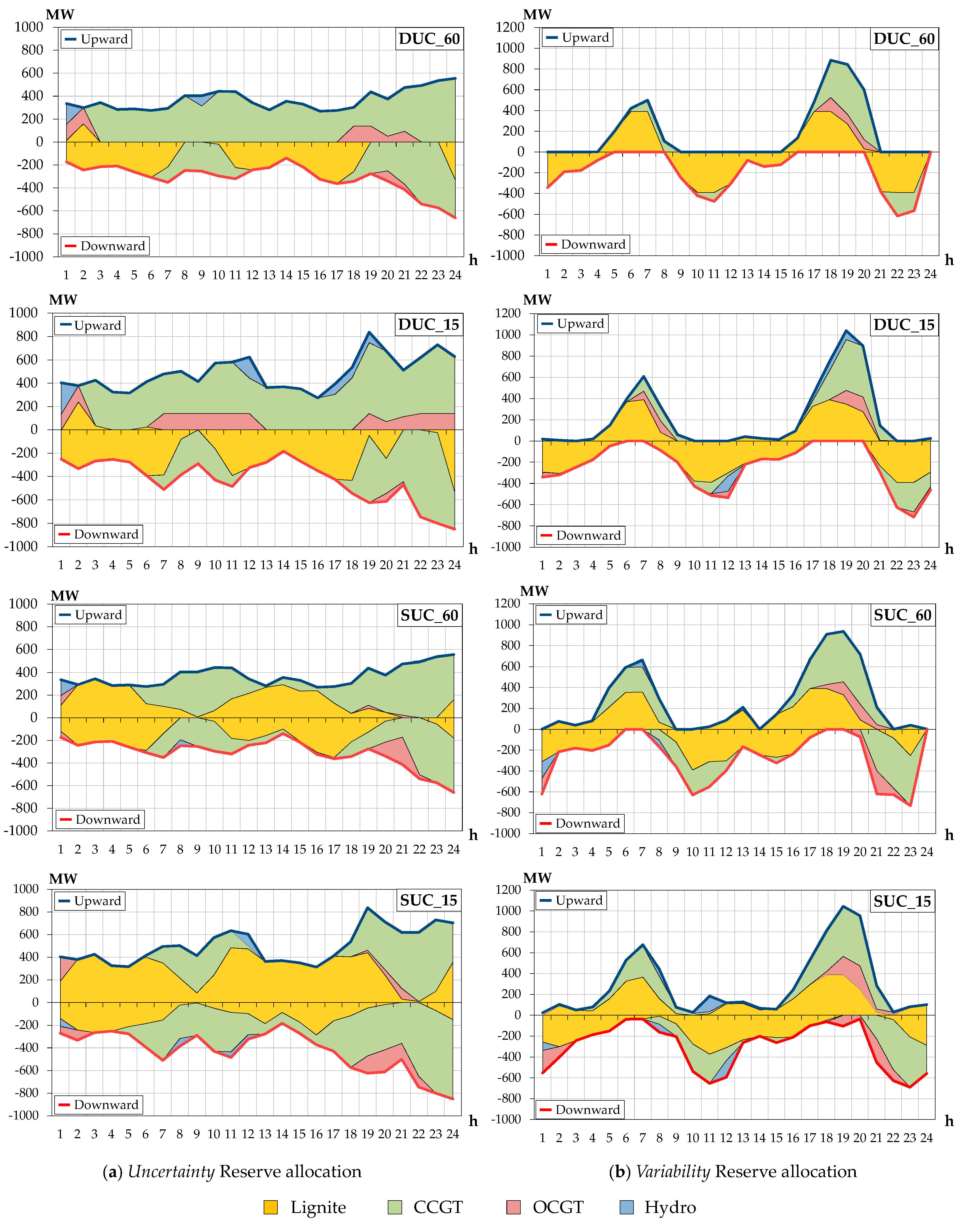
Each UC policy (SUC_15, SUC_60, DUC_15, DUC_60) is tested against all RTD modes (RTD_SI, RTD_LA_1, RTD_LA_4, RTD_SI_Var, RTD_Oneshot), with each RTD mode having a 15-min time-step and solved for any separate net load scenario considered in UC. The results focus on uncertainty and variability reserve allocation, total expected costs, power balance violations (load shedding or wind spillage), and certain features relative to the functionality of the RTD mode executed.

4. Scenario Generation

The load and wind power scenarios are calculated via a data-driven scenario generation method presented in [52], that uses historic load and wind power forecast errors of the Greek power system for the year 2013. The initial dataset contains min-to-min load and wind power measurements of the Greek interconnected power system, as well as hourly day-ahead load and wind power forecasts, provided by the Greek TSO [58] for year 2013. The wind power measurements and day-ahead forecasts have been doubled in order to consider a case with increased wind generation. Then, the 15-min load and wind forecast errors are determined, as the difference between measurements (15-min averages) and forecasts, and classified based on certain qualitative criteria. The load forecast errors are classified into lead time and time-of-day classes, and the wind forecast errors into lead time and wind forecast level classes; for each class element the Empirical Cumulative Distribution Function (ECDF) of forecast errors is calculated.

The scenario generation technique considers the temporal correlation of the forecasted time series, using the Gaussian copula approach presented in [59,60] and further explored in [61]. More specifically, the following procedure is performed separately for the generation of load and wind power scenarios. For each day, 500 random realizations are generated from a multivariate normal distribution generator using a covariance matrix. An inverse transform method for sampling is then applied to the appropriate ECDF of the forecast errors to calculate 500 respective error scenarios. A scenario reduction technique is subsequently employed to attain computational tractability, based on the probabilistic distance (Kantorovich distance), using the fast forward selection algorithm as presented in [62]. Three load error and three wind error scenarios are obtained for each day, along with their probabilities of occurrence; the respective load and wind power scenarios are calculated by adding the forecast error scenarios to the relevant point forecasts. Finally, each load scenario is combined with each wind scenario into a respective net load (load minus wind) scenario, with probability of occurrence equal to the product of probabilities of the two associated scenarios.

Figure 2 presents the nine quarterly net load scenarios and their probabilities obtained in the above context for the representative daily scheduling horizon of this case study, along with the hourly day-ahead net load forecast. Regarding the cases SUC_60 and DUC_60 (hourly real-time resolution t), it is noted that the respective hourly averages of the scenarios presented in Figure 2 are utilized.

5. Results and Discussion

5.1. Determination and Allocation of Reserves

The following Figure 3 presents the hourly uncertainty (left column diagrams) and variability (right column diagrams) reserves determined by each UC policy (DUC_60, DUC_15, SUC_60, SUC_15), for the upward (positive y-axis) and downward (negative y-axis) directions. The allocation of the reserves to the various unit categories (lignite, CCGT, OCGT, hydro) is also depicted in each diagram, with different color per unit category.

5.1.1. Determination and Allocation of the Uncertainty Reserve

As can be seen in Figure 3a, a similar profile of the system uncertainty reserve requirements (i.e., blue and red lines) is noticed in all UC policies, throughout the daily scheduling horizon. The uncertainty reserves generally increase in both directions as we move to the end of the scheduling horizon, and especially in the noon hours 18–24. This is in part due to the larger forecast errors expected as the lead-time between the day-ahead forecast and the relevant dispatch hour is increased. Additionally, the overall requirements are almost identical in DUC_60 and SUC_60 policies, and very similar in DUC_15 and SUC_15 policies, thanks to the accurate/comparable methodologies of quantifying the reserves in both the deterministic and stochastic approaches. Nevertheless, the utilization of real-time information in the latter policies (DUC_15, SUC_15) provides with increased requirements as compared to the former policies (DUC_60, SUC_60); that is, the uncertainty reserves in DUC_15 (SUC_15) have been quantified greater by 33% (36.5%) in the upward direction and 37% (39%) in the downward direction as compared to DUC_60 or SUC_60 (aggregated in a daily level). This is due to the fact that the DUC_15 and SUC_15 policies reveal potential large intra-hourly (15-min) forecast errors which are not captured by the respective hourly net load averages utilized in DUC_60 or SUC_60, while SUC_15 additionally considers the operational conditions of covering such errors at its second stage. The increase of uncertainty reserve in DUC_15 or SUC_15 is more evident in times of steep net load ramping, e.g., in hour 19 where the lower and higher values of the real (15-min) net load scenarios within said hour differ significantly from the relevant hourly point forecast (see Figure 2/hour 19). The opposite (i.e., similar uncertainty reserves in all policies) can be noticed in times of peaks or valleys of the net load, e.g., in the morning hour 9 where the real (15-min) net load scenarios considered in SUC_15 and DUC_15 do not deviate substantially from their respective hourly averages considered in SUC_60 and DUC_60 (see Figure 2/hour 9).

Most notably, the allocation of the uncertainty reserves to the various resources differs at a great extent between the stochastic and deterministic approaches. As illustrated in Figure 3a, DUC_60 and DUC_15 allocate the upward requirements mainly to more expensive CCGT, OCGT and hydro units. This is because these units (a) submit lower uncertainty reserve offers; (b) are optimally loaded at an intermediate capacity factor (CCGTs) or close to technical minimum (OCGT and hydro units), thus having enough headroom for upward reserve contribution; and (c) have lower commitment costs (OCGT and hydro units) which allow for their commitment (close to their technical minimum) during peak hours in order to contribute to upward uncertainty reserve. However, the deterministic approach does not take into account the cost of actual deployment of the uncertainty reserve by such higher-cost units in case a high net load scenario actually realizes. Instead, the lignite units are scheduled at (or close to) their available capacity, undertaking almost zero up uncertainty reserves.

In contrast, SUC_60 and SUC_15 allocate a great portion of the upward uncertainty reserve to the lignite units as can be seen in Figure 3a, despite their higher uncertainty reserve offers and the fact that such allocation often drives down their economic energy schedule from capacity; the upward reserve awards of CCGT, OCGT and hydro units are reduced equivalently in these policies. This is due to the fact that the stochastic policies also consider the deployment (energy) cost of the uncertainty reserve at the second stage, which is apparently lower in the case of lignite production. The expectation of lower deployment costs in the stochastic cases is actually confirmed in many real-time intervals when we proceed to RTD. For example, the total energy cost in the last 15-min interval of hour 18, scenario 7 (probability 0.09) and RTD case RTD_LA_4 is 48,172 € for DUC_15 and 47,652 € for SUC_15. The cost in the deterministic case is inflated mainly by an additional hydro unit committed (with zero start-up cost) for the provision of 90 MW of upward uncertainty reserve at the day-ahead stage (see Figure 3a/DUC_15/hour 18), the greater portion of which is actually dispatched at high cost in RTD.

The opposite observation can be made in the downward direction, namely the stochastic policies procure downward uncertainty reserve from higher-cost resources than the deterministic policies, since the deployment of downward uncertainty reserve is considered as a negative cost (revenue) for the TSO in objective function (1). Overall, the stochastic policies tend to commit lower cost units; in order to hedge against all possible scenarios in RTD, they reduce the capacity factor of lignite units and increase the capacity factor of CCGTs in a way that both upward and downward uncertainty and variability reserves are covered mainly by these units, avoiding (wherever possible) the commitment of higher cost production.

Finally, another positive feature of the stochastic policies is the higher correlation between the uncertainty reserve awards allocated at the day-ahead UC stage and the uncertainty reserve actually deployed by the corresponding units per scenario s in RTD. That is, in the stochastic policies, the deployment of the uncertainty reserve in RTD tends to take place from resources that were actually scheduled (and therefore remunerated) to provide the uncertainty reserve, as compared to the deterministic policies where such correlation is looser. This is depicted in the following Figure 4, which provides the correlation coefficient between the procured uncertainty reserve at the day-ahead stage in each direction (i.e., variables $r_{ih}^{{unc}^{up}}, r_{ih}^{{unc}^{dn}}$ in objective (1)) and the deployed one in RTD (i.e., variables $r_{it}^{{unc}^{up}}, r_{it}^{{unc}^{dn}}$ in (44) per scenario s), for all UC-RTD combinations executed.

5.1.2. Determination and Allocation of the Variability Reserve

A similar profile of the variability reserve requirements can also be noticed among all UC policies in Figure 3b. The variability reserve requirements are sizeable during (a) the night hours 21–4 and morning hours 10–12 in the downward direction; and (b) the early morning hours 6–8 and afternoon hours 17–20 in the upward direction, due to the respective net load ramps occurring in these hours (see Figure 2). The variability reserves increase from DUC_60 to DUC_15, SUC_60 and SUC_15, by 21%, 53% and 65%, respectively, in the upward direction, and 36%, 59% and 76% in the downward direction (aggregated in a daily level). The increase in the 15 min-based policies as compared to the corresponding 60 min-based policies is due to the fact that the former policies reveal potential large intra-hourly net load movements which are not captured by the hourly average movements utilized in the latter policies; the increase is more evident in times of steep net load ramping, like hour 19 in the upward direction and hour 12 in the downward direction. Moreover, the increase in the stochastic policies as compared to the deterministic ones is due to the fact that the former determine the variability reserve requirements through the actual output variations of the resources at the second stage, while the latter simply allocate the pre-determined requirements to the eligible resources. For example, the stochastic policies take into account a possible unit’s output increase in parallel with another unit’s output decrease (in the same interval of the second stage) when determining the upward and downward variability requirements, something which is apparently ignored in the deterministic cases.

With regard to the allocation of the variability reserve, both the deterministic and the stochastic policies generally award lower-cost units (e.g., a great portion is allocated to lignite units in all policies, as depicted in Figure 3b), since lower-cost resources have lower ramp rates and offer the variability reserve at a respective lower price in this case study. There are certain hours however, where the deterministic policies award higher-cost units than the stochastic ones, disregarding the (implicit) deployment cost of the variability reserve in case of high ramp outcomes in RTD, as also observed in [53]. For example, in hour 19, DUC_15 commits one OCGT and one higher-cost hydro unit to allocate a certain portion of the upward variability reserve (see Figure 3b/DUC_15/hour 19), while SUC_15 commits two OCGT units instead (despite their higher start-up cost). As a result, when we proceed e.g., in RTD case RTD_LA_4 and the first 15-min interval of hour 19, both DUC_15 and SUC_15 are able to cope with the high net load ramp outcomes in all scenarios, however the expected energy cost (i.e., cost attained over all scenarios executed in RTD, weighted by the respective scenario probabilities) is 49,143 € for DUC_15 and 48,909 € for SUC_15.

Most notably, the higher ramping capability of flexible resources is valued more and awarded accordingly, as the real-time ramping needs of the system are revealed at the UC scheduling stage; that is, by adopting finer time resolution for the variability reserve from DUC_60 to DUC_15 or SUC_60 to SUC_15.

Table 2. Variability reserve allocation: Comparison between DUC_60 and DUC_15 policies.

Hour 17	DUC_60	DUC_15
Up variability res. requir. (MW)	482.8	424.5 (t1: 66 t2: 64.5 t3: 117 t4: 177) 2
Lignite contrib. (MW)	390 {13} 1	325.5 {13} 1 (t1: 66 t2: 64.5 t3: 97.5 t4: 97.5) 2
CCGT contrib. (MW)	92.8 {1} 1	49.5 {1} 1 (t1: 0 t2: 0 t3: 19.5 t4: 30) 2
Hydro contrib. (MW)	-	49.5 {1} 1 (t1: 0 t2: 0 t3: 0 t4: 49.5) 2
Power balance violation in RTD_SI 3 (MWh)	t1: 0 t2: 0 t3: 0 t4: 2	t1: 0 t2: 0 t3: 0 t4: 0

¹ Within braces: Number of committed units; ² Within parenthesis: Variability reserve requirement or award determined per 15-min interval in case DUC_15; ³ Determined as ${\displaystyle \sum _{s\in S}{\pi }_s\cdot \left(l_{ts}^{Sh}+w_{ts}^{Sp}\right)/4}$ per 15-min interval t.

presents an explanatory example for hour 17, comparing DUC_60 and DUC_15 policies. In DUC_60, the more economical (in terms of variability reserve offers) lignite units are awarded 390 MW of upward reserve based on their maximum hourly ramp capability (13 units·0.5 MW/min·60 min), the rest being allocated to one CCGT unit. In DUC_15, however, the “real” ramping requirements revealed are mainly concentrated in the two latter 15-min intervals of hour 17 (i.e., 117 and 177 MW). The share of lignite units is now reduced (325.5 MW), since the slower lignite resources become ramp limited in each of the two latter intervals (13 units·0.5 MW/min·15 min = 97.5 MW) based on constraint (38). The same also applies for the CCGT unit award for the fourth interval (1 unit·2 MW/min·15 min = 30 MW), and the remaining variability reserves are now allocated to a more expensive but faster hydro unit. The result in RTD (e.g., case RTD_SI in the last row of Table 2) is an average expected power balance violation of 2 MWh in the last 15-min interval of hour 17 for DUC_60 policy; this violation and the relevant price spike is avoided in DUC_15. Note that the power balance violation occurring in RTD in DUC_60 is solely due to the ramp inability of the committed resources to follow the large increase of the net load during the fourth real-time interval, and not due to any capacity shortage (i.e., the committed capacity is enough to cover the net load in t₄). Finally, similar observations can be made in the downward direction between DUC_60 and DUC_15 (e.g., hour 21/Figure 3b), and also between SUC_60 and SUC_15 policies.

5.2. Total Expected Costs

Figure 5a provides the total costs incurred in each UC policy and respective RTD mode for the daily scheduling horizon in question. An additional UC policy is considered in this figure, named DUC, which completely disregards the variability reserve, for comparison purposes. The total cost in each UC-RTD combination consists of (a) the expected energy cost in RTD, determined as the sum of the energy costs of all scenarios executed in RTD weighted by the respective scenario probabilities; (b) the cost of uncertainty and variability reserve procurement at the day-ahead stage; (c) the commitment cost; and (d) the cost penalizing power balance violations (load shedding and wind spillage) occurring in RTD, determined again as the sum of the penalty costs of all scenarios executed in RTD weighted by the respective scenario probabilities. As observed in Figure 5a, the total costs in this case study decrease in the order DUC, DUC_60, DUC_15, SUC_60 and SUC_15, while for each specific UC policy the costs decrease in the order RTD_SI, RTD_LA_1, RTD_LA_4 or RTD_SI_Var and RTD_Oneshot. Cost reductions in the 15 min-based policies as compared to the respective 60 min-based policies in Figure 5a are achieved thanks to the reduction of ramp shortages in RTD, as a result of the increased and more accurate reserve scheduling discussed in the previous Sections. Cost reductions in the stochastic policies as compared to the deterministic ones also include the decreased deployment cost of the uncertainty reserve in RTD. Finally, as intuitively expected, the longer the look-ahead optimization horizon in RTD, the more efficient dispatch is achieved, which again leads to the reduction of ramp shortages and relevant price spikes in RTD. It should be noted that the benefits of SUC_15 over SUC_60, and DUC_15 over DUC_60 are not so evident in mode RTD_Oneshot, but this is actually not a real-world case as mentioned before; in contrast, the benefits increase in RTD modes with limited look-ahead capability as depicted in Figure 5a.

Notably, the efficiency of RTD_SI_Var (utilization of the variability reserve in RTD) is comparable with the efficiency of RTD_LA_4 (more than RTD_LA_1) for any UC policy (except DUC, where no variability reserve is considered), despite the fact that the variability reserve requirements cover the expected net load variations between two (and not four) successive real-time intervals. This is because the variability reserves are determined in UC so as to cover the maximum net load variations among all scenarios, and are not re-configured in RTD based on the expected variations in each specific scenario executed. Thus, the variability reserves are somehow increased in each specific scenario executed in RTD_SI_Var and lead to more efficient results in this constrained case study.

The system reliability achieved in the various cases is better illustrated in Figure 6, which provides the daily power balance violations (load shedding and wind spillage) in each UC-RTD combination. For each combination, the range of the daily violations occurred among all scenarios executed in RTD (high-low diagram) is provided. Note in the stochastic policies, that although the same scenarios considered in UC are also utilized in RTD, violations do incur in RTD. In SUC_60, this is in part due to the coarser (hourly) time resolution used at its second stage as compared to the 15 min resolution of RTD (as already discussed). Another factor for both SUC_60 and SUC_15 is the limited look-ahead horizon in RTD as compared to the daily scheduling horizon utilized at the second stage of these policies. The only RTD mode that resembles the second stage of SUC_15 is RTD_Oneshot, where very small violations are observed in certain scenarios as per Figure 6; such violations remained also unhedged by the least-cost dispatch determined at the second stage of SUC_15.

In fact, the limited look-ahead optimization horizon in RTD may deteriorate the reliability achieved in the stochastic policies under certain circumstances. Figure 5b presents the total costs attained in a second case study, which considers larger start-up costs for the CCGT units. In this case, the SUC policies avoid to commit the most expensive CCGT unit, which is—contrariwise—committed in the deterministic policies in hours 17–22 in order to contribute to upward variability reserves. Instead, SUC policies reduce the capacity factor of the committed lignite units (from technical maximum) and increase the capacity factor of the committed CCGT units (to maintain power balance), in a way that the overall ramp headroom in the upward direction during said hours 17–22 is able to meet the steep net load increase for all scenarios at the second stage. However, when we proceed to RTD, the economic lignite units are dispatched at (or close to) their maximum capacity in the beginning of said period in contrary to the second stage results of SUC, since the limited look-ahead horizon of previous RTD intervals fails to detect the increasing needs for upward ramping towards following intervals and produce a similar dispatch with the second stage of SUC. The result is an augmentation of ramp (and not capacity) shortages in RTD, and an overall higher cost as compared to the deterministic policies, for all RTD modes with limited look-ahead horizon (see Figure 5b). The only RTD mode that provides better results for the stochastic policies in this case study is RTD_Oneshot, which resembles the dispatch outcome attained in the second stage of SUC, as previously discussed. Overall, this case study shows that, in their effort to avoid high commitment costs or expensive (thus often also fast) generation committed for the provision of reserves, the stochastic UC policies may provide a more “risky” schedule, which, combined with the limited optimization horizon in RTD, may ultimately result in ramp shortages and higher overall costs.

5.3. Computational Requirements

All UC policies were modeled in GAMS© 24.3.3 [63] and solved using solver CPLEX 12.6 [64]. The net load scenarios and the deterministic uncertainty and variability reserve requirements were calculated using MATLAB© R2013b [65]. The case studies were executed on a 2.6-GHz Intel Quad Core i7 processor with 16 GB of RAM, running 64-bit Windows. The deterministic UC policies provided proven optimal solutions, while the stochastic UC policies were solved with a relative optimality gap of 0.05%.

Table 3. Size of UC models and total execution times.

UC Policy	Constraints	Continuous Variables	Binary Variables	Total Execution Time (s)
DUC_60	18,249	12,715	5014	16
DUC_15	24,729	19,051	5014	38.5
SUC_60	107,568	55,915	5014	240
SUC_15	343,440	185,515	5014	3307

summarizes the computational complexity and the total execution time for each UC policy examined in this section (base case).

The results demonstrate that both DUC_60 and DUC_15 provide proven optimal solutions at fast execution times, thus their application to medium-sized systems like the Greek power system or even larger power systems comprising several tens of units is practicable. Computational complexity somehow increases in SUC_60, but still a reasonable execution time is attained for a limited number of scenarios, as in this case study. Notwithstanding the benefits of SUC_15, the computational burden and the execution time increases drastically due to the scenarios utilized and the finer time resolution at the second stage for both the uncertainty and variability reserve. Advances in optimization software and computer hardware are required for more practical execution times to be attained in SUC_15 policy. Nevertheless, decreasing the scheduling horizon in the order of 4–6 h (or less, in the case of RTUC), implementing a less detailed modeling for the generating unit operating states, or using other techniques [46] like grouping generating units by type, considering must-run units, or implementing “warm-start” strategies, shall reduce execution times to a great extent.

6. Conclusions

This paper presented and evaluated different deterministic and stochastic day-ahead UC policies, with focus on the determination, allocation and deployment of reserves, by making an explicit distinction between the uncertainty and the variability reserve. The main conclusions are:

(a)

The inclusion of the variability reserve in the day-ahead UC reduces the possibility for ramp shortages and relevant price spikes in RTD and enhances system reliability.

(b)

The consideration of higher time resolution when procuring the reserves in both the deterministic and stochastic approaches, according to the proposed multi-timing scheduling concept, reveals potential large intra-hourly net load forecast errors and variations, and often awards faster resources, leading again in increased system reliability and lower expected costs.

(c)

The comparable formulations developed between the deterministic and stochastic policies derive similar overall reserve requirements, however the (upward) reserves tend to be allocated in lower cost units in the stochastic policies, considering their relative deployment cost. Also, the correlation between procured (in UC) and deployed (in RTD) uncertainty reserves has proven higher in the stochastic cases.

(d)

The utilization of the variability reserve in RTD brings efficiencies in managing the steep net load movements, which can be comparable with the use of look-ahead functionality in RTD.

(e)

Finally, in their effort to avoid high commitment costs or expensive (thus often also fast) generation committed for the provision of reserves, the stochastic UC policies may occasionally provide a more “risky” schedule, which, combined with the limited optimization horizon in RTD, may ultimately deteriorate reliability in real-time conditions.

Notwithstanding the contributions of this paper, certain issues can be further investigated in our ongoing research, among which are the following: (a) incorporation of the transmission network constraints; (b) consideration of techniques that will help to reduce the execution times of the SUC model (especially case SUC_15), e.g., decomposition techniques; and (c) execution of the case study for the days of a larger representative period (e.g., yearly simulation) to attain more robust results.

References

1. Trombe, P.-J.; Pinson, P.; Madsen, H. A general probabilistic forecasting framework for offshore wind power fluctuations. Energies 2012, 5, 621–657. [Google Scholar] [CrossRef] [Green Version]
2. Sperati, S.; Alessandrini, S.; Pinson, P.; Kariniotakis, G. The “Weather Intelligence for Renewable Energies” benchmarking exercise on short-term forecasting of wind and solar power generation. Energies 2015, 8, 9594–9619. [Google Scholar] [CrossRef] [Green Version]
3. Hong, Y.-Y.; Yu, T.-H.; Liu, C.-Y. Hour-ahead wind speed and power forecasting using empirical mode decomposition. Energies 2013, 6, 6137–6152. [Google Scholar] [CrossRef]
4. Cadenas, E.; Rivera, W.; Campos-Amezcua, R.; Heard, C. Wind speed prediction using a univariate ARIMA model and a multivariate NARX model. Energies 2016, 9, 109. [Google Scholar] [CrossRef]
5. Osório, G.J.; Gonçalves, J.N.D.L.; Lujano-Rojas, J.M.; Catalão, J.P.S. Enhanced forecasting approach for electricity market prices and wind power data series in the short-term. Energies 2016, 9, 693. [Google Scholar] [CrossRef]
6. Doherty, R.; O’Malley, M. A new approach to quantify reserve demand in systems with significant installed wind capacity. IEEE Trans. Power Syst. 2005, 20, 587–595. [Google Scholar] [CrossRef]
7. Lange, M. On the uncertainty of wind power predictions-analysis of the forecast accuracy and statistical distribution of errors. J. Sol. Energy Eng. 2005, 127, 177–184. [Google Scholar] [CrossRef]
8. Ela, E.; O’Malley, M. Studying the variability and uncertainty impacts of variable generation at multiple timescales. IEEE Trans. Power Syst. 2012, 27, 1324–1333. [Google Scholar] [CrossRef]
9. Deane, J.P.; Drayton, G.; Gallachóir, B.P.Ó. The impact of sub-hourly modelling in power systems with significant levels of renewable generation. Appl. Energy 2014, 113, 152–158. [Google Scholar] [CrossRef]
10. Pandzic, H.; Dvorkin, Y.; Wang, Y.; Qiu, T.; Kirschen, D.S. Effect of time resolution on unit commitment decisions in systems with high wind penetration. In Proceedings of the 2014 IEEE PES General Meeting, Washington, DC, USA, 27–31 July 2014.
11. Ummels, B.C.; Gibescu, M.; Pelgrum, E.; Kling, W.L.; Brand, A.J. Impacts of wind power on thermal generation unit commitment and dispatch. IEEE Trans. Energy Convers. 2007, 22, 44–51. [Google Scholar] [CrossRef]
12. GE Energy. Western Wind and Solar Integration Study; National Renewable Energy Laboratory (NREL): Golden, CO, USA, 2010. [Google Scholar]
13. Enernex Corporation. Eastern Wind Integration and Transmission Study; National Renewable Energy Laboratory (NREL): Golden, CO, USA, 2011. [Google Scholar]
14. Ecofys. All Island TSO Facilitation of Renewables Studies; EirGrid Plc: Dublin, Ireland, 2010. [Google Scholar]
15. Ela, E.; Milligan, M.; Parsons, B.; Lew, D.; Corbus, D. The evolution of wind power integration studies: Past, present, future. In Proceedings of the 2009 IEEE PES General Meeting, Calgary, AB, Canada, 26–30 July 2009.
16. Wood, A.J.; Wollenberg, B.F. Power Generation, Operation, Control; Wiley: New York, NY, USA, 1984. [Google Scholar]
17. Isemonger, A.G. The evolving design of RTO ancillary service markets. Energy Policy 2009, 37, 150–157. [Google Scholar] [CrossRef]
18. Wu, T.; Rothleder, M.; Alaywan, Z.; Papalexopoulos, A.D. Pricing energy and ancillary services in integrated market systems by an optimal power flow. IEEE Trans. Power Syst. 2004, 19, 339–347. [Google Scholar] [CrossRef]
19. ISO New England. ISO New England Operating Procedure No. 8 Operating Reserve and Regulation. Available online: https://www.iso-ne.com/static-assets/documents/rules_proceds/operating/isone/op8/op8_rto_final.pdf (accessed on 30 November 2016).
20. PJM. PJM Manual 11. Energy & Ancillary Services Market Operations. Available online: http://www.pjm.com/~/media/documents/manuals/m11.ashx (accessed on 30 November 2016).
21. Makarov, Y.V.; Loutan, C.; Jian, M.; Mello, P. Operational impacts of wind generation on California power systems. IEEE Trans. Power Syst. 2009, 24, 1039–1050. [Google Scholar] [CrossRef]
22. Kwon, K.; Park, H.; Lyu, J.-K.; Park, J.-K. Cost analysis method for estimating dynamic reserve considering uncertainties in supply and demand. Energies 2016, 9, 845. [Google Scholar] [CrossRef]
23. Mauer, C.; Krahl, S.; Weber, H. Dimensioning of secondary and tertiary control reserve by probabilistic methods. Eur. Trans. Electr. Power 2009, 19, 544–552. [Google Scholar] [CrossRef]
24. Matos, M.A.; Bessa, R.J. Setting the operation reserve using probabilistic wind power forecasts. IEEE Trans. Power Syst. 2011, 26, 594–603. [Google Scholar] [CrossRef]
25. Menemenlis, N.; Huneault, M.; Robitaille, A. Computation of dynamic operating balance reserve for wind power integration for the time-horizon 1–48 hours. IEEE Trans. Sustain. Energy 2012, 3, 692–702. [Google Scholar] [CrossRef]
26. Bakirtzis, E.A.; Biskas, P.N.; Bakirtzis, A.G. Dynamic reserves quantification for variable time resolution scheduling. In Proceedings of the IEEE PowerTech 2015, Eindhoven, The Netherlands, 29 June–2 July 2015.
27. Bakirtzis, E.A.; Biskas, P.N.; Labridis, D.P.; Bakirtzis, A.G. Multiple time resolution unit commitment for short-term operations scheduling under high renewable penetration. IEEE Trans. Power Syst. 2014, 29, 149–159. [Google Scholar] [CrossRef]
28. Holttinen, H.; Milligan, M.; Kirby, B.; Acker, T.; Neimane, V.; Molinski, T. Using standard deviation as a measure of increased operational reserve requirement for wind power. Wind Eng. 2008, 32, 355–378. [Google Scholar] [CrossRef]
29. Holttinen, H.; Milligan, M.; Ela, E.; Menemenlis, N.; Dobschinski, J.; Rawn, B.; Bessa, R.J.; Flynn, D.; Gomez-Lazaro, E.; Detlefsen, N.K. Methodologies to determine operating reserves due to increased wind power. IEEE Trans. Sustain. Energy 2012, 3, 713–723. [Google Scholar] [CrossRef]
30. Ela, E.; Milligan, M.; Kirby, B. Operating Reserves and Variable Generation; National Renewable Energy Laboratory (NREL): Golden, CO, USA, 2011. [Google Scholar]
31. Marneris, I.G.; Biskas, P.N.; Bakirtzis, E.A. An integrated scheduling approach to underpin flexibility in European power systems. IEEE Trans. Sustain. Energy 2016, 7, 647–657. [Google Scholar] [CrossRef]
32. Xu, L.; Tretheway, D. Flexible Ramping Products; California ISO: Folsom, CA, USA, 2014. [Google Scholar]
33. Navid, N.; Rosenwald, G. Ramp Capability Product Design for MISO Markets. Available online: https://www.misoenergy.org/Library/Repository/Communication%20Material/Key%20Presentations%20and%20Whitepapers/Ramp%20Product%20Conceptual%20Design%20Whitepaper.pdf (accessed on 30 November 2016).
34. Abdul-Rahman, K.H.; Alarian, H.; Rothleder, M.; Ristanovic, P. Enhanced system reliability using flexible ramp constraint in CAISO market. In Proceedings of the IEEE PES General Meeting, San Diego, CA, USA, 22–26 July 2012.
35. Navid, N.; Rosenwald, G. Market solutions for managing ramp flexibility with high penetration of renewable resource. IEEE Trans. Sustain. Energy 2012, 3, 784–790. [Google Scholar] [CrossRef]
36. Krad, I.; Ibanez, E.; Ela, E. Quantifying the potential impacts of flexibility reserve on power system operations. In Proceedings of the 2015 Seventh Annual IEEE Green Technology Conference, New Orleans, LA, USA, 15–17 April 2015.
37. Ela, E.; O’Malley, M. Scheduling and pricing for expected ramp capability in real-time power markets. IEEE Trans. Power Syst. 2016, 31, 1681–1691. [Google Scholar] [CrossRef]
38. Wang, C.; Luh, P.B.; Navid, N. Requirement design for a reliable and efficient ramp capability product. In Proceedings of the IEEE PES General Meeting, Vancouver, BC, Canada, 21–25 July 2013.
39. Birge, J.R.; Leveaux, F.V. Introduction to Stochastic Programming; Springer: Berlin, Germany, 1997. [Google Scholar]
40. Bouffard, F.; Galiana, F.D.; Conejo, A.J. Market-clearing with stochastic security—Part II: Case studies. IEEE Trans. Power Syst. 2005, 20, 1827–1835. [Google Scholar] [CrossRef]
41. Ruiz, P.A.; Philbrick, C.R.; Zak, E.; Cheung, K.W.; Sauer, P.W. Uncertainty management in the unit commitment problem. IEEE Trans. Power Syst. 2009, 24, 642–651. [Google Scholar] [CrossRef]
42. Ruiz, P.A.; Philbrick, C.R.; Sauer, P.W. Modeling approaches for computational cost reduction in stochastic unit commitment formulations. IEEE Trans. Power Syst. 2010, 25, 588–589. [Google Scholar] [CrossRef]
43. Papavasiliou, A.; Oren, S.S.; O’Neill, R.P. Reserve requirements for wind power integration: A scenario-based stochastic programming framework. IEEE Trans. Power Syst. 2011, 26, 2197–2206. [Google Scholar] [CrossRef]
44. Papavasiliou, A.; Oren, S.S. Multi-area stochastic unit commitment for high wind penetration in a transmission constrained network. Oper. Res. 2013, 61, 578–592. [Google Scholar] [CrossRef]
45. Bouffard, F.; Galiana, F.D. Stochastic security for operations planning with significant wind power generation. IEEE Trans. Power Syst. 2008, 23, 306–316. [Google Scholar] [CrossRef]
46. Morales, J.M.; Conejo, A.J.; Pérez-Ruiz, J. Economic valuation of reserves in power systems with high penetration of wind power. IEEE Trans. Power Syst. 2009, 24, 900–910. [Google Scholar] [CrossRef]
47. Sahin, C.; Shahidehpour, M.; Erkmen, I. Allocation of hourly reserve versus demand response for security-constrained scheduling of stochastic wind energy. IEEE Trans. Sustain. Energy 2013, 4, 219–228. [Google Scholar] [CrossRef]
48. Wang, B.; Liu, X.; Zhu, F.; Hu, X.; Ji, W.; Yang, S.; Wang, K.; Feng, S. Unit commitment model considering flexible scheduling of demand response for high wind integration. Energies 2015, 8, 13688–13709. [Google Scholar] [CrossRef]
49. Wu, H.; Shahidehpour, M.; Alabdulwahab, A.; Abusorrah, A. Thermal generation flexibility with ramping costs and hourly demand response in stochastic security-constrained scheduling of variable energy sources. IEEE Trans. Power Syst. 2015, 30, 2955–2964. [Google Scholar] [CrossRef]
50. Tuohy, A.; Meibom, P.; Denny, E.; O’Malley, M. Unit commitment for systems with significant wind penetration. IEEE Trans. Power Syst. 2009, 24, 592–601. [Google Scholar] [CrossRef] [Green Version]
51. Sturt, A.; Strbac, G. Efficient stochastic scheduling for simulation of wind-integrated power systems. IEEE Trans. Power Syst. 2012, 27, 323–334. [Google Scholar] [CrossRef]
52. Bakirtzis, E.A.; Biskas, P.N. Multiple time resolution stochastic scheduling for systems with high renewable penetration. IEEE Trans. Power Syst. 2016. [Google Scholar] [CrossRef]
53. Wang, B.; Hobbs, B.F. Real-time markets for flexiramp: A stochastic unit-commitment-based analysis. IEEE Trans. Power Syst. 2016, 31, 846–860. [Google Scholar] [CrossRef]
54. Wang, B.; Hobbs, B.F. A flexible ramping product: Can it help real-time dispatch markets approach the stochastic dispatch ideal? Elect. Power Syst. Res. 2014, 109, 128–140. [Google Scholar] [CrossRef]
55. Lee, Y.-Y.; Baldick, R. A frequency-constrained stochastic economic dispatch model. IEEE Trans. Power Syst. 2013, 28, 2301–2312. [Google Scholar] [CrossRef]
56. Simoglou, C.K.; Biskas, P.N.; Bakirtzis, A.G. Optimal self-scheduling of a thermal producer in short-term electricity markets by MILP. IEEE Trans. Power Syst. 2010, 25, 1965–1977. [Google Scholar] [CrossRef]
57. Price, J.E.; Rothleder, M. Recognition of extended dispatch horizons in California’s energy markets. In Proceedings of the IEEE PES General Meeting, Detroit, MI, USA, 24–28 July 2011.
58. Hellenic Independent Power Transmission Operator. Available online: http://www.admie.gr/nc/en/home/ (accessed on 30 November 2016).
59. Pinson, P.; Madsen, H.; Nielsen, H.A.; Papaefthymiou, G.; Klöckl, B. From probabilistic forecasts to statistical scenarios of short-term wind power production. Wind Energy 2009, 12, 51–62. [Google Scholar] [CrossRef] [Green Version]
60. Pinson, P.; Girard, R. Evaluating the quality of scenarios of short-term wind power generation. Appl. Energy 2012, 96, 12–20. [Google Scholar] [CrossRef] [Green Version]
61. Ma, X.-Y.; Sun, Y.-Z.; Fang, H.-L. Scenario generation of wind power based on statistical uncertainty and variability. IEEE Trans. Power Syst. 2013, 4, 894–904. [Google Scholar] [CrossRef]
62. Conejo, A.J.; Carrión, M.; Morales, J.M. Decision Making under Uncertainty in Electricity Markets; Springer-Science Business Media: Berlin, Germany, 2010. [Google Scholar]
63. General Algebraic Modeling System (GAMS). Available online: http://www.gams.com/ (accessed on 30 November 2016).
64. International Business Machines Corporation (IBM) CPLEX Optimizer. Available online: http://www-01.ibm.com/software/integration/optimization/cplex-optimizer (accessed on 30 November 2016).
65. The MathWorks Inc. MATLAB Version R2013b Natick; The MathWorks Inc.: Natick, MA, USA, 2013. [Google Scholar]
Figure 1. Definition of uncertainty and variability reserves.
Energies 10 00140 g001
Figure 2. Net load: Day-ahead forecast and real-time scenarios with probabilities.
Energies 10 00140 g002
Figure 3. Uncertainty and variability reserve allocation per unit category in various UC policies.
Energies 10 00140 g003
Figure 4. Correlation between procured and deployed uncertainty reserves by the eligible units.
Energies 10 00140 g004
Figure 5. Total daily costs for all UC-RTD combinations.
Energies 10 00140 g005
Figure 6. Daily power balance violations for all UC-RTD combinations.
Energies 10 00140 g006