Investigation of the Flow Characteristics of Methane Hydrate Slurries with Low Flow Rates

Abstract

Gas hydrate blockage in pipelines during offshore production becomes a major problem with increasing water depth. In this work, a series of experiments on gas hydrate formation in a flow loop was performed with low flow rates of 0.33, 0.66, and 0.88 m/s; the effects of the initial subcooling, flow rate, pressure, and morphology were investigated for methane hydrate formation in the flow loop. The results indicate that the differential pressure drop (ΔP) across two ends of the horizontal straight pipe increases with increasing hydrate concentration at the early stage of gas hydrate formation. When the flow rates of hydrate fluid are low, the higher the subcooling is, the faster the transition of the hydrates macrostructures. Gas hydrates can agglomerate, and sludge hydrates appear at subcoolings of 6.5 and 8.5 °C. The difference between the ΔP values at different flow rates is small, and there is no obvious influence of the flow rates on ΔP. Three hydrate macrostructures were observed: slurry-like, sludge-like, and their transition. When the initial pressure is 8.0 MPa, large methane hydrate blockages appear at the gas hydrate concentration of approximately 7%. Based on the gas–liquid two-phase flow model, a correlation between the gas hydrate concentration and the value of ΔP is also presented. These results can enrich the kinetic data of gas hydrate formation and agglomeration and provide guidance for oil and gas transportation in pipelines.

1. Introduction

Gas hydrates are non-stoichiometric clathrate crystalline compounds and they form by water and gas molecules such as methane, ethane, or propane at high-pressure and low-temperature conditions [1]. Water molecules are hydrogen-bonded so as to form cage structures that are stabilized by filling with gas molecules.

Gas hydrates, primarily those of methane, mainly exist in sea floor deposits and permafrost. In order to overcome the problem posed by the shortage of onshore oil and gas resources, increasingly more attention is being paid to marine gas hydrates as a potential energy source [2]. However, their use can also cause some problems such as geological collapse of the seafloor owing to gas hydrate dissociation and greenhouse effects caused by the release of methane to the atmosphere [3,4]. Most commonly, gas hydrates can form in the pipeline during oil and gas transportation and result in security risks.

Hammerschmidt [5] first reported the formation of hydrates in gas pipelines. As the petroleum industry is now moving towards deep water, gas hydrates easily form under such conditions and aggregate in the pipe, eventually blocking the pipeline. Thus, the issue of pipeline blockage by gas hydrates must be resolved. Several studies have also investigated this topic [6,7]. The use of gas hydrate inhibitors is the most common method to prevent hydrate blockage [8].

Thermodynamic hydrate inhibitors have been widely used, such as methanol, glycol, and electrolytes. These inhibitors are effective; however, they must be used in large concentrations, which adversely affect the profits of a project [9]. The cost of using methanol per day for hydrate inhibition is about US $740,000 worldwide [10]. In addition, some thermodynamic hydrate inhibitors such as methanol are harmful to the environment.

A new type of gas hydrate inhibitor, low-dosage hydrate inhibitors (LDHIs), has been proposed to prevent hydrate nucleation and growth [11]. There are two kinds of LDHIs: anti-agglomerants (AAs) and kinetic hydrate inhibitors (KHIs). Although neither of these can change the thermodynamic conditions required for gas hydrate formation, they can prevent and delay gas hydrate nucleation or growth. These inhibitors are used at low concentrations, often less than 1 wt % [12,13,14,15,16,17], and have been used in many fields [18].

Gas hydrates with effective LDHIs can flow in pipelines without blocking the pipe or agglomerating together. This method is the so-called risk control method. Thus, the study of gas hydrate formation is very important to solving the problem of hydrate blockage.

Some researchers have studied natural gas/water systems with flow assurance. However, most of these studies were conducted using high-pressure autoclaves [19,20]. Joshi [10] presented an analysis of hydrate formation experiments to discover the mechanism of gas hydrate blockage in a pipeline with high water cut systems. In their work, methane hydrate slurries were investigated with flow rates of 1 m/s or more. Gas hydrate formation was divided into three regions and the gas hydrate concentration could be used as an indicator of hydrate plugging. Andersson and Gudmundsson [21] reported a frictional pressure drop of water–methane and a gas mixture hydrate slurry in turbulent flow, which was identical to the frictional pressure drop of pure water. However, the frictional pressure drop increased with increasing gas hydrate concentration in the laminar region. Zerpa et al. [22] proposed a three-phase flow model and compared the model results against the experimental data in an industrial flow loop.

Some research focused on the gas/oil/water system in both a high-pressure autoclave and a flow loop [23,24,25]. Webb et al. [26] investigated in situ methane hydrate formation from water-in-crude oil emulsions in a high-pressure rheology apparatus. The viscosity of the hydrate slurry attained the maximum value in 20 min, and then it began to decay. Sinquin et al. [27] pointed out that when hydrates form in pipelines, the pressure drop is decided by the friction factor and apparent viscosity in the turbulent and laminar flow regimes, respectively. Yan et al. [28] investigated the characteristics of gas hydrate slurry with initial water cuts of 5–30 vol %. Their experimental results showed that the hydrate slurry presented obvious shear-thinning behavior when the hydrate volume fraction increased. Fidel-Dufour et al. [29] examined the crystallization process of the methane hydrate/water/dodecane system and found that the viscosity of hydrates slurry increased before reaching a constant value and again increased after achieving the contestant value; this behavior is dependent on the water content. Moradpour et al. [30] predicted the viscosity of a water/oil/hydrate mixture using a bimodal model, which considered the mixture’s viscosity as its binary components’ viscosity.

Few data are available on the flow assurance in pipelines for natural gas/water systems, especially for low flow rate systems. Low flow rates sometimes appear in the oil and gas field because of the terrain constraints or for unpredicted reasons. It is necessary to obtain more data on the flow properties of hydrate particles so as to be able to control the flow assurance in pipelines. In this work, the flow characteristics and rheological properties of methane gas hydrate slurries in a pipeline were examined with the initial water cuts of 48 vol % at different flow rates (0.33, 0.66, and 0.88 m/s) and subcoolings (4.5, 6.5, and 8.5 °C). The pressure drop, hydrate concentrations, and morphologies of the hydrate slurry at different stages were investigated. Using the experimental data obtained, an empirical rheological model based on the Lockhart–Martinelli gas–liquid two-phase flow equation was proposed to describe the viscosity at different hydrate concentrations.

2. Materials and Experimental Section

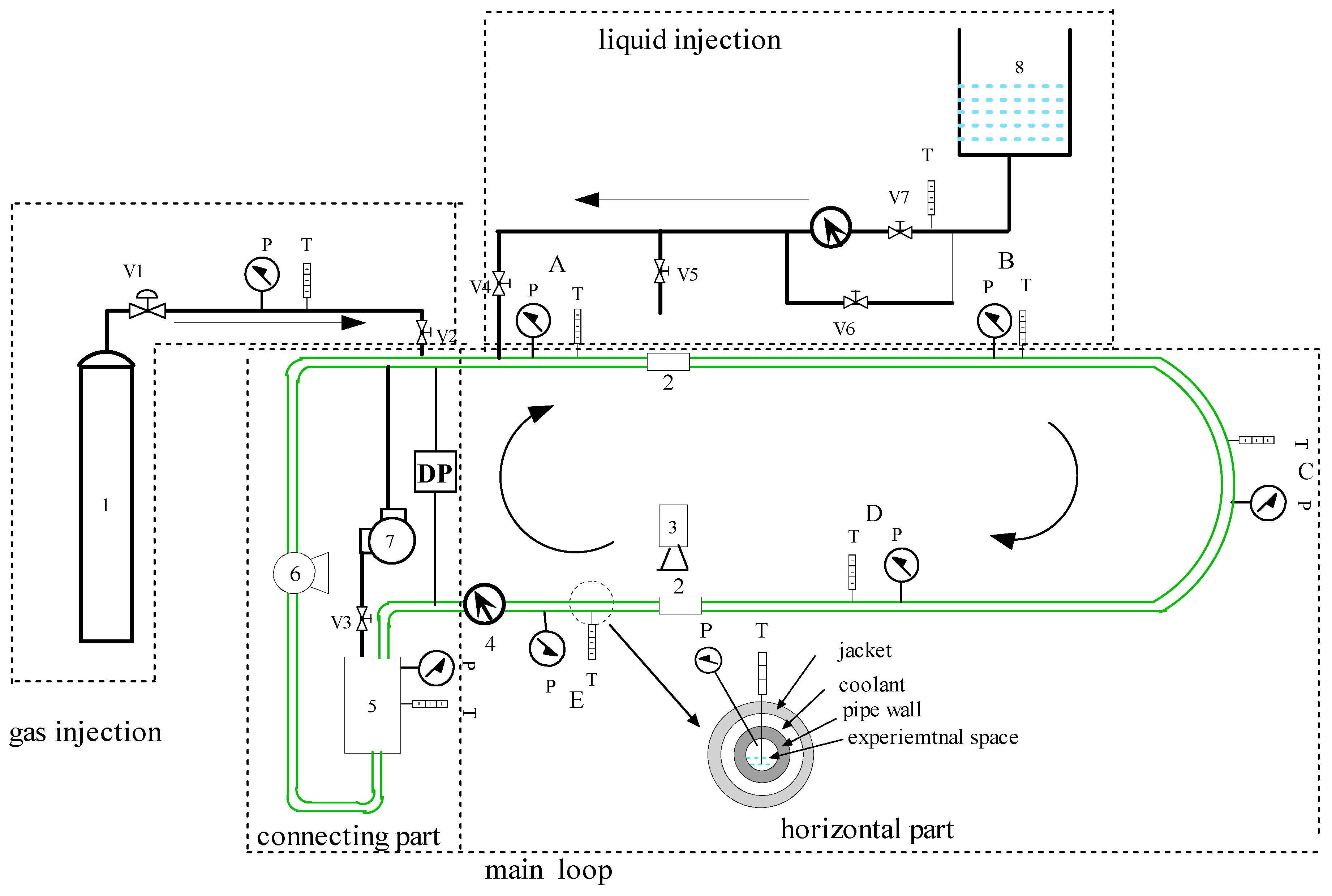
2.1. Experimental Flow Loop Description

All experiments were performed in a flow loop (Figure 1). The flow loop has three sections: gas and liquid injection sections, and the main loop. These sections are made of 316 stainless steel. The main loop was 51.85 m long, with an internal pipe diameter of 2.54 cm, including a horizontal part of 42.35 m and a connection part. There were three transparent visual windows, two of them located at the middle of the horizontal straight pipe and the other at the vertical section that was not used in this experiment, and hence not shown in Figure 1. One of the visual windows was equipped with a digital camera. The maximum designed pressure that the flow loop could be pressurized with was 15 MPa. The temperature of the flow loop was controlled in the range from −20 to 50 °C with the help of a refrigerating unit.

Eight thermocouples (±0.15 °C) were used to measure the temperature of the fluid in the different sections of the flow loop; the temperature sensing elements of four of them were located at one-third of the pipe cross section and the others at two-thirds of the cross section. Eight pressure sensors (±0.25% full scale, FS) and a differential pressure transducers (±0.065% FS) were used to measure the gas pressure in the loop and differential pressure across the inlet and outlet of the horizontal pipe. The flow rate was measured by a C7B5D0B1AD1E1Z mass flow meter (Xian Dongfeng Machinery & Electronic Co., Ltd. Xi’an, China) with an accuracy of ±0.065% FS. A 3DXP-2.2/10-30-T7 piston pump (Chongqing Pump Industry Co., Ltd., Chongqing, China, this pump was custom-designed to minimize shear effect on hydrate slurries and influence of operation mode) was used to recycle the fluid with a maximum reciprocating time of 338 min⁻¹. The data of temperature, pressure, flow rate, and differential pressure throughout the experiments were collected using a data-acquisition system at an interval of 10 s.

Temperature profiles in the main loop are shown in Figure 2, derived from the reliability experiments conducted using this setup. The temperatures are similar to each other in different sections of the loop, the temperature differences are small, and the change is the same. The first increase in the temperature occurs at about 500 s and is attributed to the starting of the liquid pump. For ease of understanding, the temperature and pressure at point E are chosen as the representatives for the following analysis.

2.2. Experimental Procedure and Materials

Before conducting the experiments, the flow loop was cleaned by flushing with pure water and was then drained by nitrogen gas. Thereafter, 15.0 L of distilled water (self-made in the lab) was charged into the loop and the system was vacuumed for 15 min. The loop was pressurized for about 3 min with methane gas (99.9% purity, Guangzhou Puyuan Gas Co., Guangzhou, China) to the desired pressure (6.3 MPa or 8 MPa in this work). Then, the temperature of the loop was decreased to 9.2 °C from room temperature at the initial gas pressure of 6.3 MPa, or to 11.6 °C at 8.0 MPa. The fluids were recycled in the loop with a flow rate of 0.18 m/s for about 1 h to saturate the liquid phases with gas. After that, the loop was repressurized to 6.3 MPa or 8.0 MPa to compensate for the pressure drop caused by temperature decrease. Then, the gas supply was cut off. The flow loop was then cooled to the desired temperatures, which would be mentioned in the specific experimental runs. At the same time, the fluid was recycled at the experimental flow rates (0.33, 0.66, or 0.88 m/s). Gas hydrate formation could be observed by visual windows or inferred by an increase in temperature or abrupt decrease in pressure. Hydrate growth occurred until the time pressure became stable or gas hydrate morphologies remained stable for more than 1 h. Finally, the flow loop temperature was increased to room temperature to dissociate the hydrates, which marked the end of the experiment.

The flow characteristics and morphology of the hydrate slurry were investigated at different subcoolings, flow rates, and initial pressures. In all experiments, to reduce the impact of accidental factors, gas hydrate were formed and dissociated, and then the experiment was repeated with this reacted solution according to the experimental procedure. The data from the repeating experiment were collected (the secondary hydrate formation method).

3. Results and Discussion

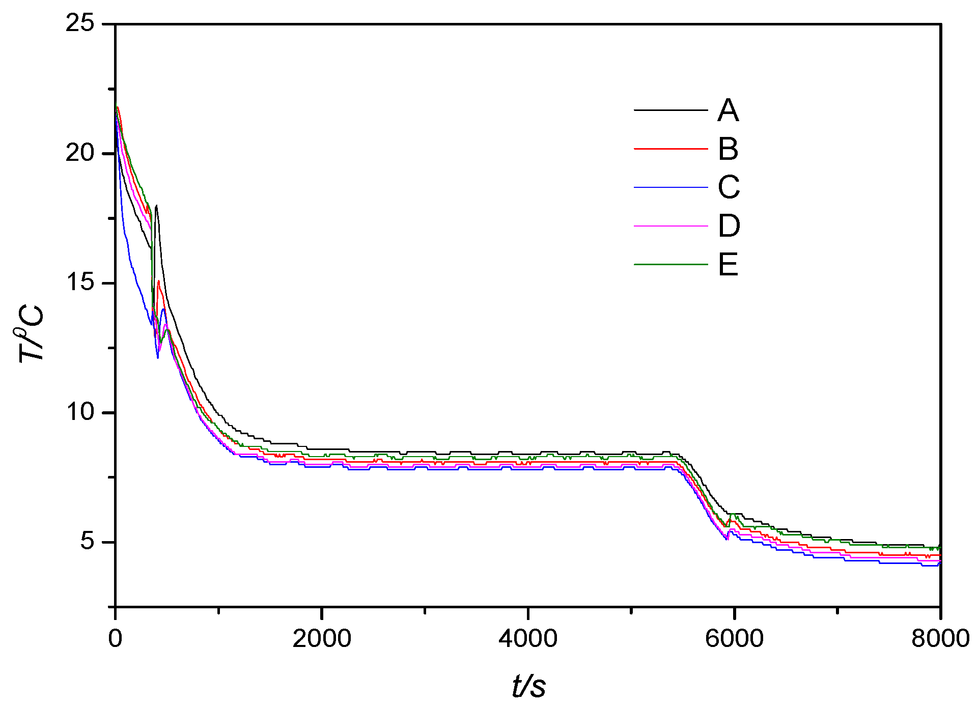
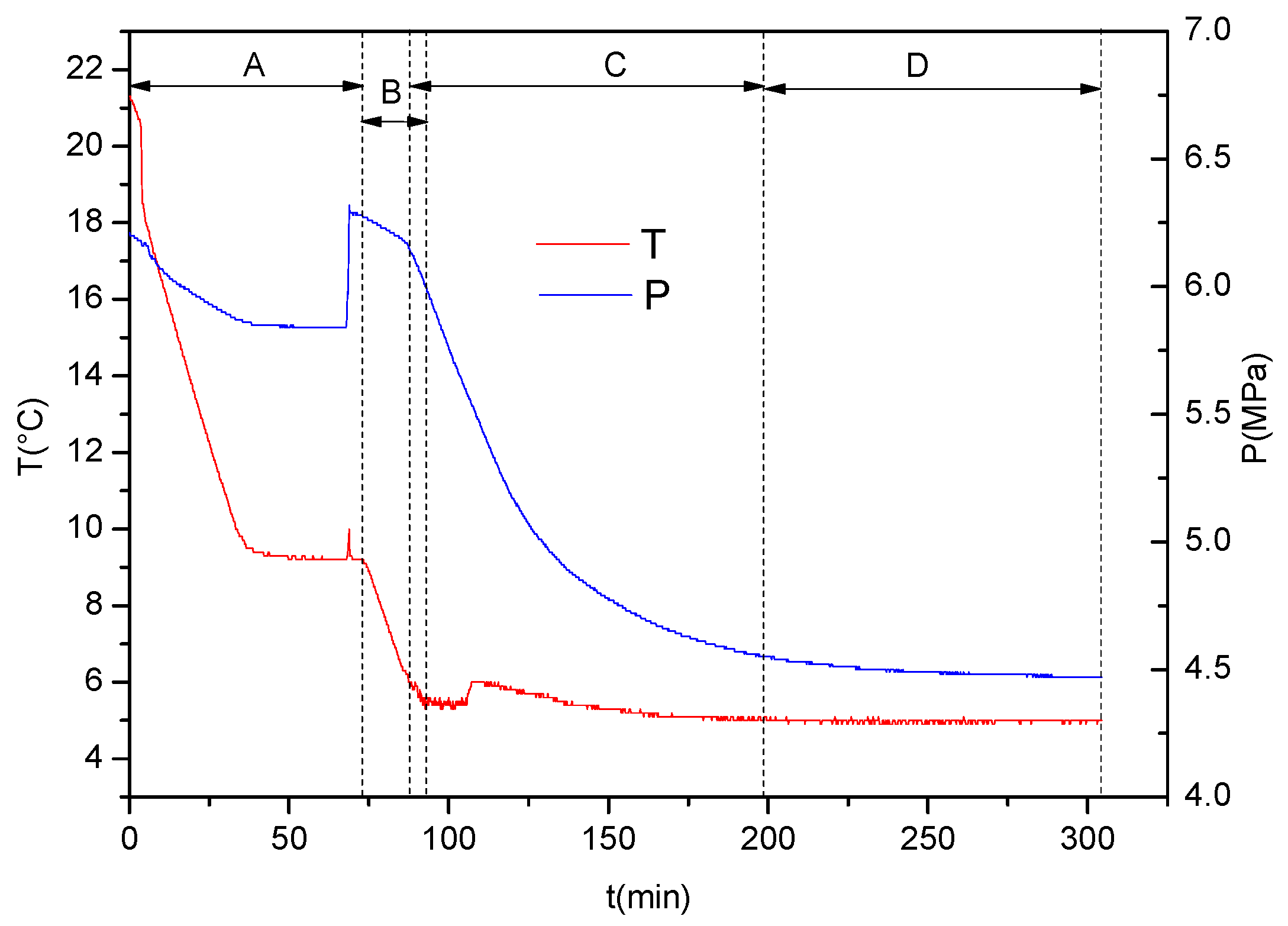
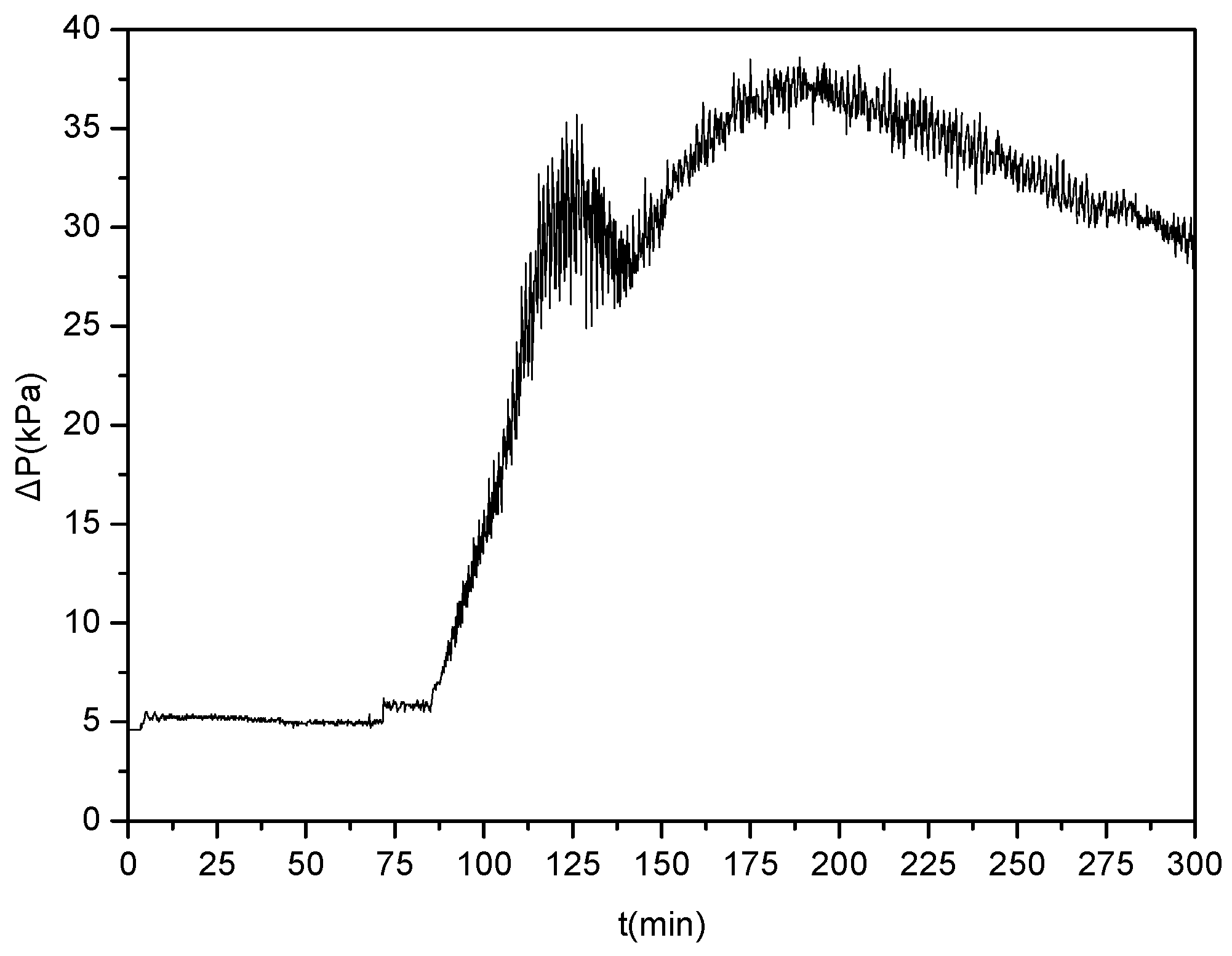
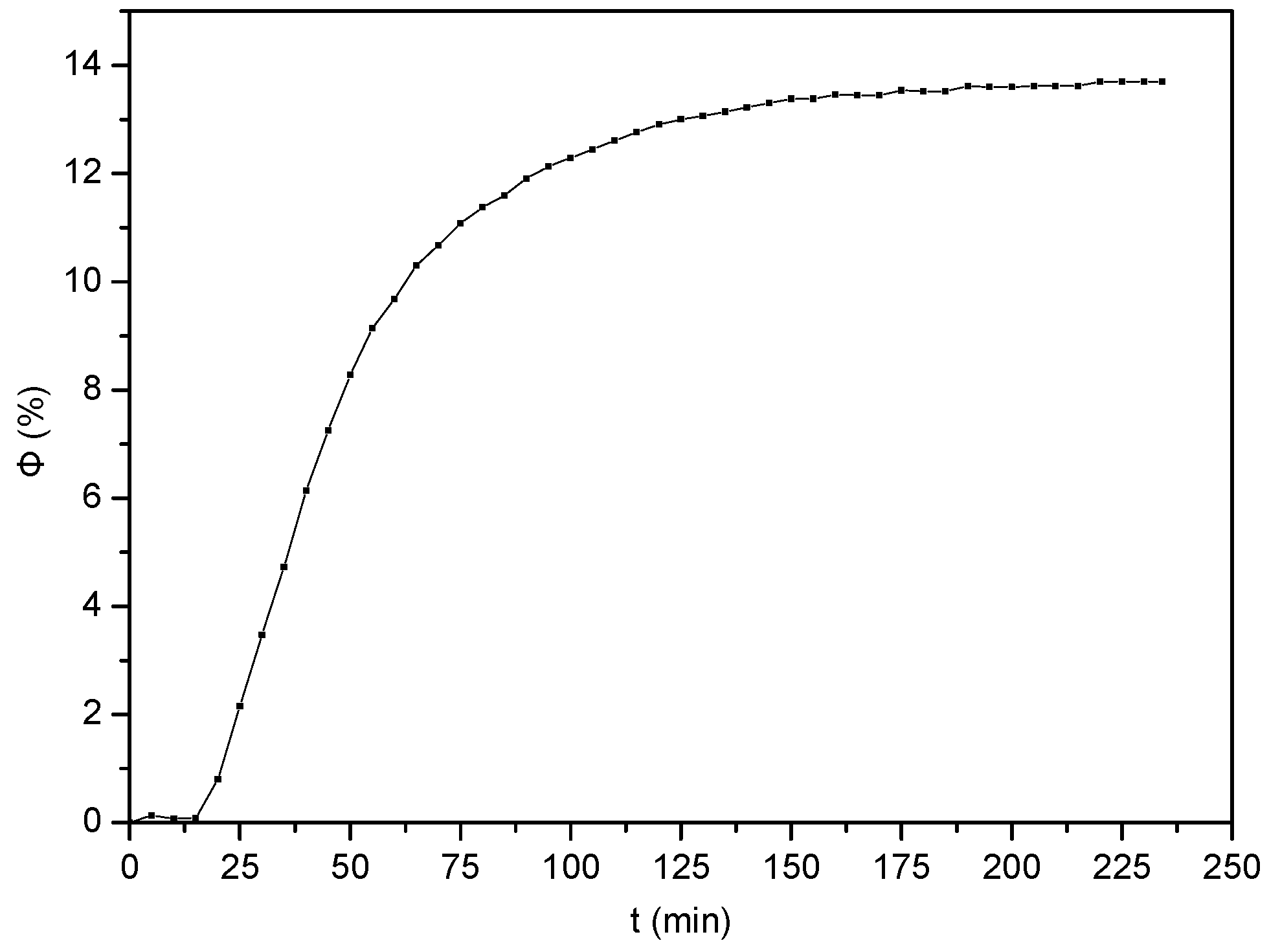
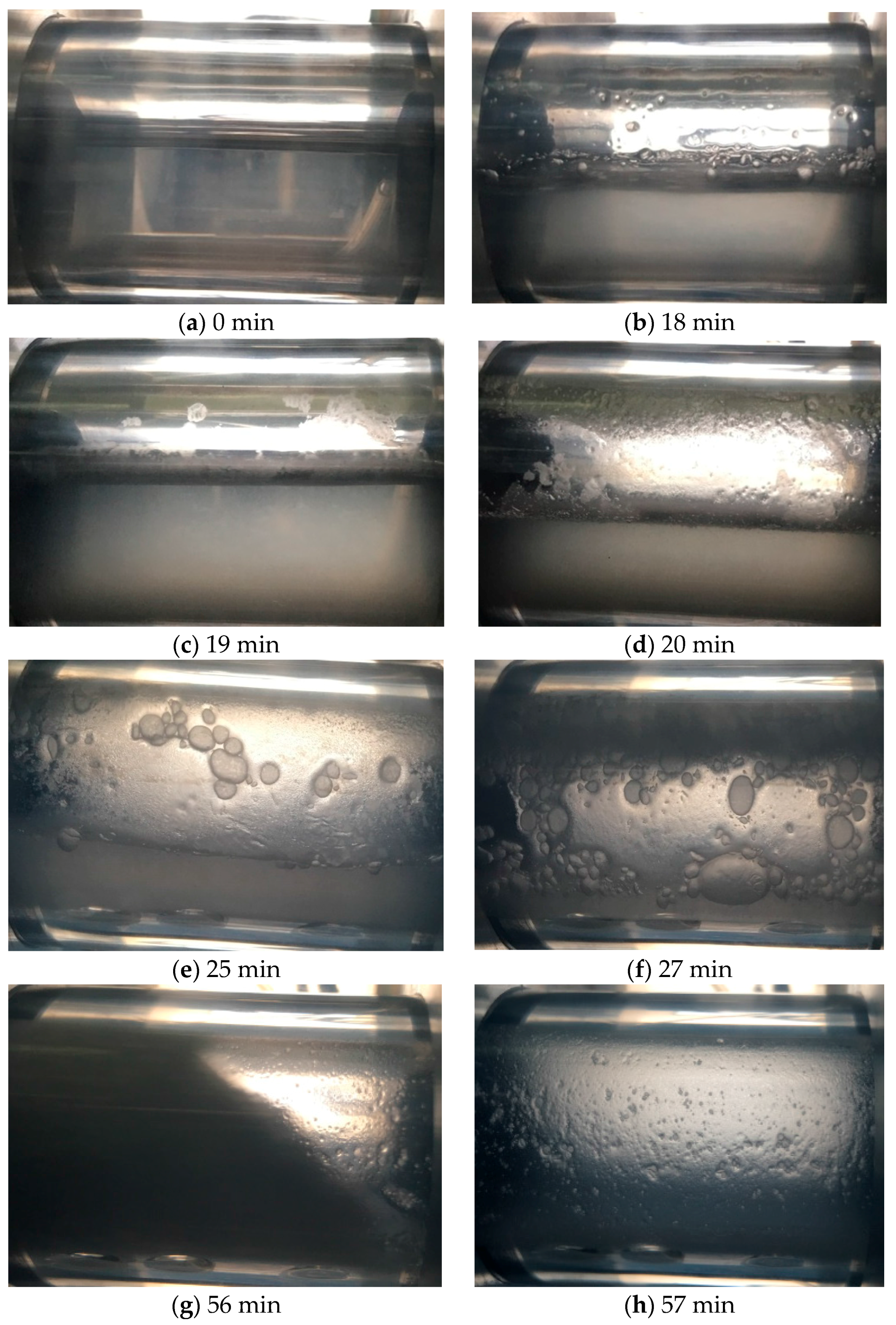
3.1. Typical Experimental Run

The typical changes of the temperature and pressure during gas hydrate formation is shown in Figure 3. Stage A was the preparation stage, which included the decrease in temperature, stabilizing of the temperature, and repressurization of the gas (to compensate for the pressure drop caused by temperature drop). In stage B, the temperature was set at 4.5 °C to promote hydrate formation. The gas hydrate formation and agglomeration occurred in stage C. The inflection point on the pressure curve and the instantaneous temperature fluctuation can indicate the onset of gas hydrate formation. Gas hydrate formation ended in stage D. At 6.3 MPa, the equilibrium temperature was approximately 9.0 °C and the subcooling temperature was 4.5 °C.

Gas hydrate formed at stage B when the temperature approached the target value of 4.5 °C; at the same time, there were obvious fluctuations in the temperature and pressure curve (Figure 3). The temperature and pressure became steady after gas hydrate formation.

The differential pressure (ΔP) was measured across the inlet and outlet of the horizontal pipe.

ΔP is an important parameter for the liquid flow system, which implies the resistance change. In the following study, ΔP was connected with gas hydrate content, so in Figure 4, the change of ΔP with elapsed time was shown, which could supply an intuitive understanding. ΔP was constant before gas hydrate formation. The fluctuation occurred 72 min after the beginning of the experiment because of the change of the flow rate from 0.18 to 0.33 m/s. ΔP immediately increased upon hydrate formation. After 190 min, the temperature and pressure became steady, and ΔP achieved the maximum value. This tendency of ΔP with elapsed time is consistent with the results reported by Joshi et al. [10] at low velocities. The up-and-down fluctuation in ΔP may be caused by the piston pump, which was designed to minimize shear on hydrate slurries and influence of the operation mode. In the experiments, the up-and-down fluctuation of ΔP still exited but was small enough, and the general change tendency with time is very clear.

After 190 min, ΔP began to decrease, and, within the next 100 min, the value of ΔP decreased by 9 kPa (24% of the maximum value). The hydrate growth and agglomeration were more violent because of the presence of more gas–liquid interfaces and gas–liquid–solid contact areas in the multiphase system, and pressure decreased rapidly after hydrate formation [31]. Webb et al. [26] reported the same variation in the viscosity using an autoclave, while Joshi et al. [10] also observed similar results for ΔP in a flow loop. Through the visual window, the changes in the morphology of the hydrate slurry could be seen, and the obvious agglomeration was observed. Thus, the drop in the ΔP value might indicate a change in the macrostructures of methane hydrate agglomeration. The main characteristics of the hydrate macrostructures can be divided into five groups: slurry-like, slush-like, powder-like, and their transition zones [32]. Slurry-like hydrate is a liquid-like mixture of particles and looks like milk. During the transition stage from slurry hydrate to slush, hydrate clusters stick together. In slush-like hydrates, hydrates form larger clusters and lumps and look like wet snow. Hydrate lumps break up during the transition from slush-like hydrates to powder-like hydrates. At the powder-like stage, hydrates are powder-like and can be easily transported [32]. Slush-like hydrates were also observed when ΔP approached the maximum value.

Methane hydrate concentration is an important parameter for a gas hydrate flow system. To determine methane hydrate concentration in the fluid, the methane volume in the gas phase is assumed to be constant (16.5 L in this work). Here, the hydrate volume concentration is expressed in terms of the conversion percentage of gas, Φ, shown in Equation (1), and the amount of dissolved methane in water is too small to be neglected:

$$\mathsf{\phi }=\frac{V_{hydrate}}{V_{hydrate}+V_{water}}\times 100\%$$

(1)

$$V_{hydrate}=M_{hydrate}(n_{gi}-n_g)/{\mathsf{\rho }}_{hydrate}$$

(2)

$$V_{water}=(15000-6M_{water}(n_{gi}-n_g))/{\mathsf{\rho }}_{water}$$

(3)

Here, V_hydrate, V_water, M_hydrate, M_water, n_gi, and n_g represent the volumes of gas hydrate and water, molecular weights of hydrate and water, and methane content in the gas phase at the start of the experiment and at time t, respectively. Methane content in the gas phase was calculated by the Soave–Redlich–Kwong equation of state using the P/T data. The hydration number of 6 is chosen and the gas hydrate formula is considered as CH₄·6H₂O [10]. The densities of the gas hydrate and water here are considered as 9.1 × 10² kg/m³ and 1.0 × 10³ kg/m³, respectively. When hydrate dissolution in water is not taken into account, the value of $V_{hydrate}+V_{water}$ varies from 15.0 L to 15.4 L, as calculated by Equations (2) and (3), which implies a maximum deviation of 2.6% from the value of the constant gas volume assumed for the experimental run shown in Figure 2. In fact, part of the hydrate would dissolve in water, and the total gas volume was between 15.0 and 15.4 L. To simplify the calculation, $V_{hydrate}+V_{water}$ were considered as 15.0 L.

The zero point of time in all figures following Figure 4 is defined as 3 min prior to the beginning of stage B in Figure 3.

Figure 5 shows changes in the calculated hydrate volume concentration with respect to the elapsed time during gas hydrate formation. After about 75 min, the slope of the Φ vs. elapsed time curve decreased, which indicated that the gas hydrate formation rate declined with the elapsed time. This meant that the gas hydrate formation rate first increased, then decreased, and, finally, approached zero. At the final stage, the gas hydrate concentration did not change any further. Combined with Figure 3 and Figure 4, in the last 110 min, temperature t and methane hydrate concentration remained constant, but the differential pressure began to drop, which also implied morphological change in gas hydrate aggregation.

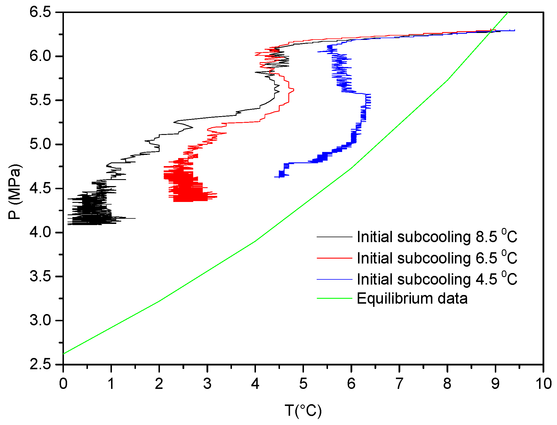
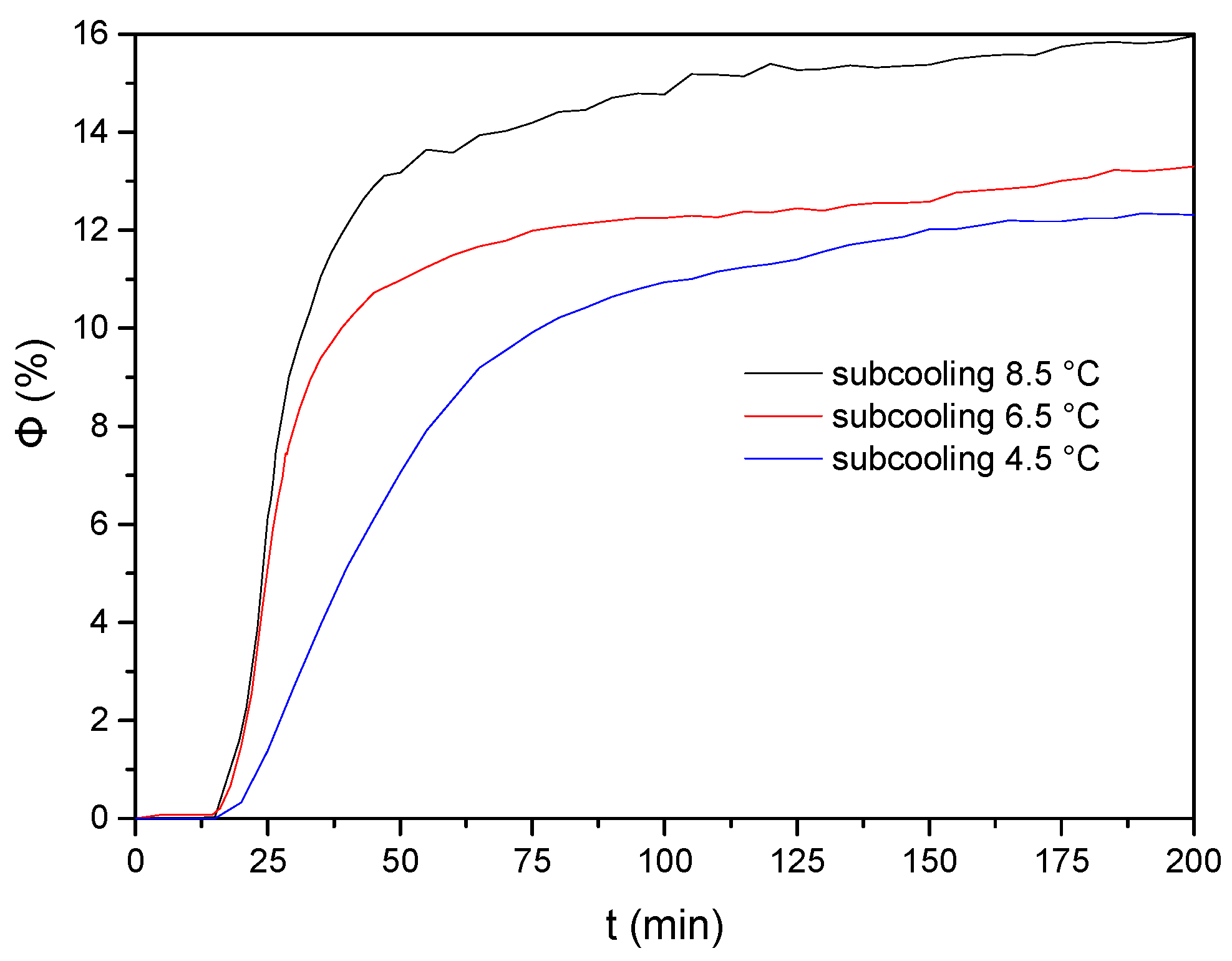
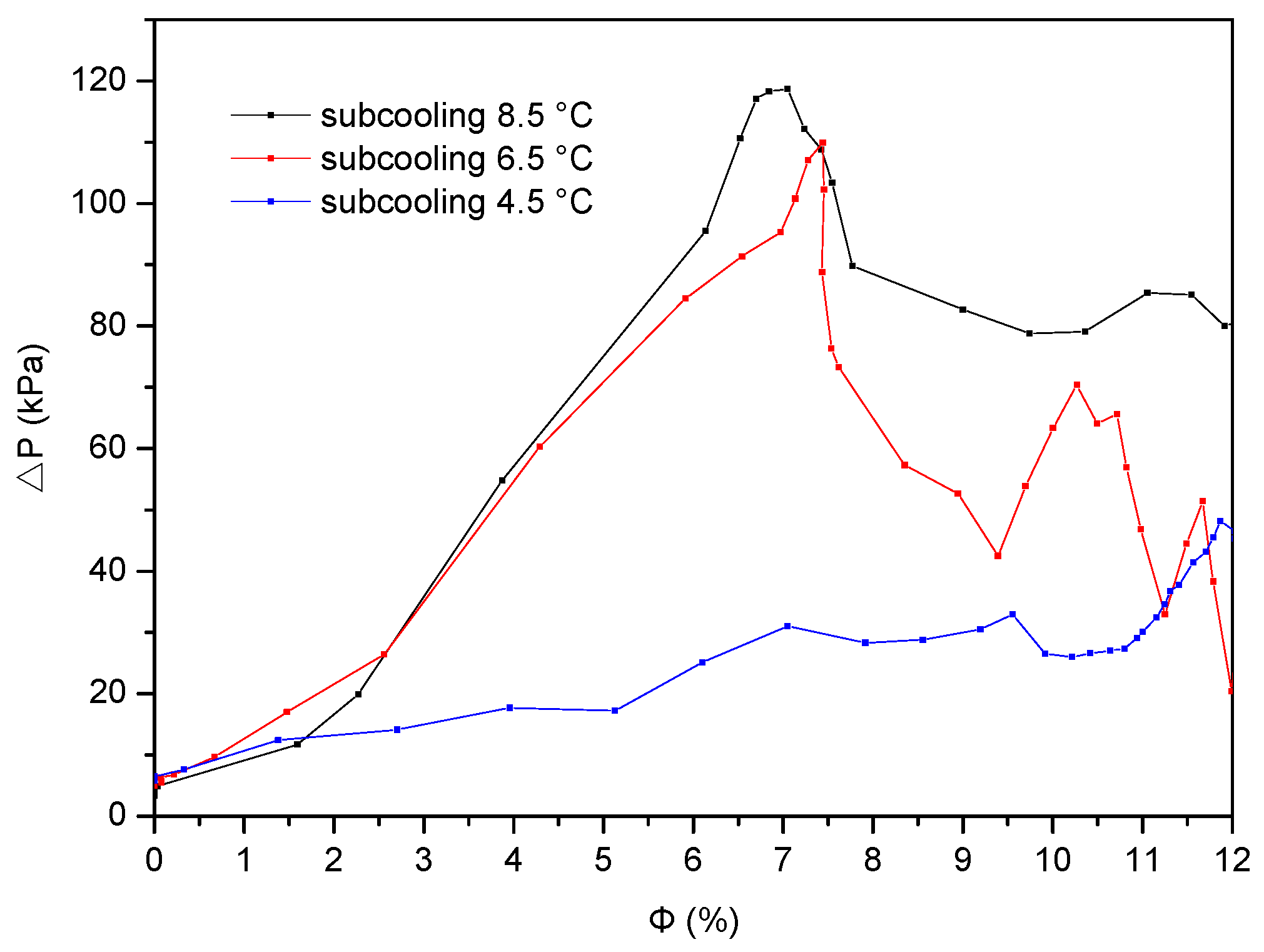
3.2. Effect of Initial Subcooling

Figure 6 shows the evolution of P and T in the experimental process. For each subcooling experiment, the initial pressure was 6.3 MPa and the flow rate was 0.33 m/s. Three initial subcoolings were examined: 4.5, 6.5, and 8.5 °C. With gas hydrate formation, subcoolings were changing with elapsed time.

The temperature and pressure changes were almost the same as those of three experimental runs with different initial subcoolings before gas hydrate formation; the temperature decreased at nearly the same rate. After gas hydrate formation, the change in pressure with temperature became different but showed the same tendency.

Figure 7 shows the change in gas hydrate concentration with elapsed time. For the initial subcoolings of 6.5 and 8.5 °C, the gas hydrate formation rate was almost the same as that at the beginning stage. This indicated that when the driving force was larger than a certain value, the difference in the gas hydrate formation rate was small if the system was cooled down at a fixed rate. When gases were progressively consumed and the target temperature was approached, the P/T value was close to the equilibrium condition and the driving force for all cases became smaller; therefore, the hydrate concentration increased with the driving force (subcoolings here) increasing at this stage.

In Figure 8, ΔP almost increased with the increase of hydrate volume concentration at a subcooling of 4.5 °C within the total experimental time, except for a small fluctuation of 9.5% in the value of Φ. However, for subcoolings of 6.5 and 8.5 °C, two turning points were observed in the curve of ΔP with Φ.

For all of the experiments were stopped at the time that pressure became stable and there was no change of gas hydrates morphologies. No obvious large agglomerates were observed for the subcooling of 4.5 °C during the experiments. With increasing subcooling, the sludge hydrates could be observed through the visual window, and, therefore, the sudden change in ΔP could be owing to changes in the hydrate macrostructures. Generally, ΔP increases with increasing Φ because the fluid macrostructure changed to a solid–liquid–gas mixture from the liquid–gas system during gas hydrate formation; as a result, the viscosity of the mixture also increased. The fluid viscosity and the friction between the pipe wall and the fluid increased with increasing hydrate concentration. When solid hydrates appeared, they attached to the pipe wall or flowed with liquid. The resistance between the pipe wall and internal friction of fluids both increased the viscosity. If the amount of gas hydrates was up to a certain extent, the fluid would lose mobility and plug the pipeline.

Progressive gas hydrate formation is beneficial to the aggregation of hydrates, but the flow of liquid is not conducive to the formation of hydrate clusters. Therefore, if the formation rate is slow, the existing hydrate clusters can be broken up, which may reduce the ΔP value. Conversely, if the formation rate is high enough, ΔP will increase. The visual window observation showed that gas hydrate particles became small and the fluid became highly viscous; however, no hydrate clusters were seen at the final stage for all experiments. As a result, ΔP had the maximum value and a small fluctuation of 9.5% was observed in the Φ value for the experiments with the initial subcooling of 4.5 °C. In Figure 8, the higher the subcooling, the faster the transition of the hydrate macrostructures, which implied that there was no obvious difference in the gas hydrate formation rate at the early stage if the subcooling was high enough, but the total gas hydrate formation rate increased with increasing subcooling.

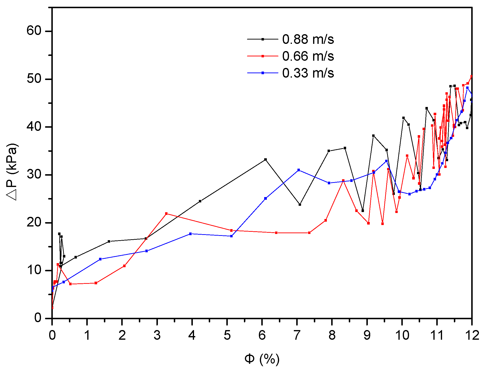
3.3. Effect of Flow Rate

For each experimental run in this section, the initial pressure was 6.3 MPa and the subcooling was 4.5 °C. The following flow rates were considered: 0.33, 0.66, and 0.88 m/s.

Figure 9 shows the effect of the three different flow rates on the value of ΔP. At different flow rates, the value of ΔP increases with increasing hydrate concentration, and, except for 0.33 m/s, a little drop in the ΔP value was observed at Φ of 9.5%; however, the ΔP value increased very quickly, which was discussed above. The difference between the values of ΔP at each flow rate was small. At the same hydrate concentration, the flow rate did not appear to be an obvious influence on the value of ΔP. The rate of temperature decrease was the same for the same target temperature at different flow rates. When all conditions were the same, except for the flow rate, ΔP increased abruptly when the hydrate concentration, Φ, was about 11% for all experimental runs. Thus, the hydrate aggregation degree might change. In the previous analysis, the drop in ΔP was thought to result from the breaking up of hydrate clusters, which made the transport of fluid easy. However, ΔP did not achieve the maximum value and had no turning point in Figure 9, which indicated that large hydrate clusters did not exist when the flow rate was higher. This may mean that the high flow rate was advantageous for fluid transportation with hydrate particles.

Induction times for gas hydrate formation at different flow rates are shown in

Table 1. Gas hydrate formation times with different flow rates at the initial pressure of 6.3 MPa and the subcooling of 4.5 °C.

No.	Flow Rate (m/s)	Induction Time (min)
1	0.88	22.5
2	0.66	21.0
3	0.33	33.8

. Although the secondary hydrate formation method was used, the gas hydrate formation induction time is arbitrary but close for the flow rates of 0.88 and 0.66 m/s; however, it was lower at 0.33 m/s. At 0.33 m/s, the induction time for gas hydrate formation was longer than that at the other rates because the disturbance and mixing of the fluids were not sufficiently intense.

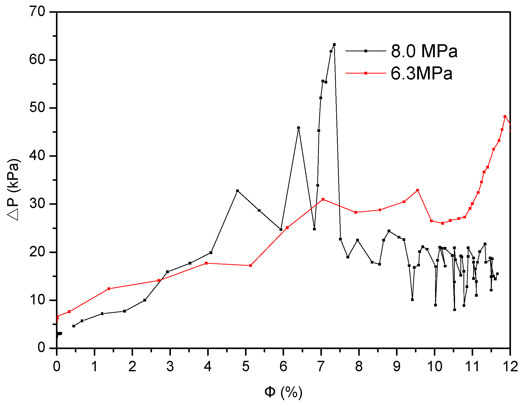
3.4. Effect of Pressure

A subcooling of 4.5 °C and a flow rate of 0.33 m/s were used to examine the effect of the initial pressure. At 8.0 MPa, hydrate blockages occurred in the pipe; thus, no additional higher pressures were examined except for the initial pressures of 6.3 and 8.0 MPa.

At an initial pressure of 8.0 MPa (Figure 10), the maximum value of ΔP was 66.1 kPa when the gas hydrate concentration was approximately 7%, and 12% methane was consumed in the gas phase, after which the value of ΔP began to drop. Large methane hydrate blockages were observed, and they moved slowly in the pipe when ΔP approached the maximum value. However, the macrostructure of the hydrates was still slush-like, more hydrates agglomerated together, and no powder-like hydrates appeared.

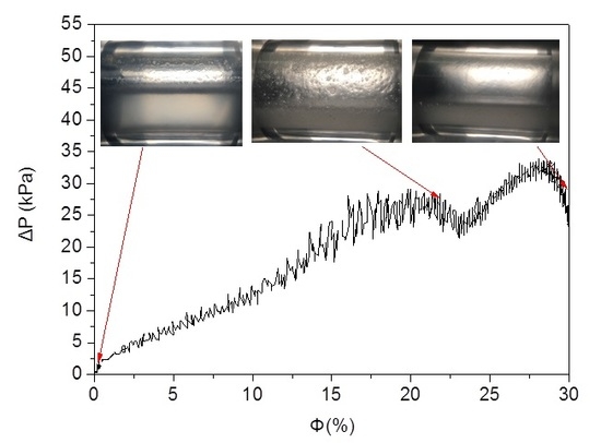
3.5. Morphologies of Gas Hydrates in the Pipe

Figure 11 shows the morphologies of gas hydrates at different formation times before the blockage occurred. For the experiment shown in Figure 11, the initial pressure was 8.0 MPa, subcooling was 4.5 °C, and flow rate was 0.33 m/s. The fluid in the pipe was clear and transparent before hydrate formation (Figure 11a). Gas hydrates formed at the gas–liquid interface during the temperature decrease, were flushed to the pipe wall (Figure 11b), and then agglomerated on the pipe wall (Figure 11c). The formed hydrates were slurry-like. Subsequently, more hydrates agglomerated and attached to the wall (Figure 11d). Hydrate lumps appeared on the wall after 25 min and became bigger (Figure 11e). As the reaction progressed, slush-like hydrates appeared (Figure 11f,g) and agglomerated together but could flow when ΔP approached the maximum value (Figure 11g). After the slush hydrate flowed away, no liquid was found at the window glass (Figure 11h). In the experimental time employed, no powder-like and transition macrostructure from slush-like to powder-like appeared.

The reaction could be summarized as follows: gas hydrates formed at the gas–liquid interface and attached to the pipe wall, or were suspended in a liquid. Then, the hydrates on the wall agglomerated and became lumps, and the fluid became slurry-like. Finally, all hydrates agglomerated together and formed slush-like agglomerates.

3.6. Pressure Drop Model

Here, the gas and liquid phases were assumed to be homogenous. The separated fluid model was used to simplify the simulation (Figure 12). Gas filled the upper space of the pipe, and the bottom of the pipe contained the liquid.

The model was based on the Lockhart–Martinelli gas–liquid two-phase flow Equations (4)–(6) [33]:

$$\frac{dp}{dz}={\mathsf{\phi }}_l^2{(\frac{dp}{dz})}_l$$

(4)

$${\mathsf{\phi }}_l^2=1+C{X}^{-1}+X^{-2}$$

(5)

$$X^2=\frac{{(\frac{dp}{dz})}_l}{{(\frac{dp}{dz})}_g}$$

(6)

where (dp/dz)_l represents the pressure drop when there is 100% liquid flow in the pipe at respective superficial velocities, and (dp/dz)_g for 100% gas; ${\mathsf{\phi }}_l^2$ and X² represents the liquid conversion coefficient and the Lockhart–Martinelli parameter, respectively. The laminar flow formulas (for the gas) and the turbulent flow formulas (for the liquid) were adopted according to the Reynolds number. Here, c was 10.

For the gas phase, (dp/dz)_g could be obtained from Equations (7) and (8) [33]:

$${(\frac{dp}{dz})}_g=\frac{{\mathsf{\lambda }}_g}{d}\frac{v_g{}^2}{2}{x}^2\frac{1}{{\mathsf{\rho }}_g}$$

(7)

$${\mathsf{\lambda }}_g=\frac{64}{{\mathrm{Re}}_g}$$

(8)

where λ_g, v_g, x, ρ_g, and Re_g represent the friction coefficient, mass flow rate, mass concentration, density, and Reynolds number for the gas, respectively, and d is the inner diameter of the pipe.

For the liquid phase, (dp/dz)_l could be obtained from Equations (9) and (10) [33,34]:

$${(\frac{dp}{dz})}_l=\frac{{\mathsf{\lambda }}_l}{d}\frac{v_l{}^2}{2}{(1-x)}^2\frac{1}{{\mathsf{\rho }}_l}$$

(9)

$${\mathsf{\lambda }}_l=\frac{64}{{\mathrm{Re}}_l}$$

(10)

where λ_l, v_l, ρ_l, and Re_l represent the friction coefficient, mass flow rate, density, and Reynolds number for the liquid, respectively.

Many empirical models are available for the friction coefficient [35]. Equation (10) was used for the liquid in this work to simplify the calculations because the flow rate was low and the viscosity would increase only when the gas hydrate was formed. In the actual operation, the viscosity of the gas hydrate slurry, an important parameter, could be used to determine the properties of the flow and pressure drop. The Thomas model [36] was used for the viscosity, and a regression equation could be obtained:

$${\mathsf{\eta }}_{\mathrm{h}}={\mathsf{\eta }}_{\mathrm{L}}(1+265.75\mathsf{\varphi }+10.05{\mathsf{\varphi }}^2+0.368{\mathrm{e}}^{30.6\mathsf{\varphi }})$$

(11)

where η_h and η_l represent the viscosities of the hydrate slurry and water, respectively.

The pressure drop before gas hydrate formation was deducted. Figure 13 shows that the experimental data matched well with the predicted value for the pressure drop, ΔP. However, when the hydrate concentration reached the turning point, the experimental values began to deviate from the predicted ones. The increasing value of ΔP might be affected by the agglomeration of gas hydrates. Thus, Equation (11) could only be used before gas hydrate agglomeration.

Equation (11) was modified as a general form of ${\mathsf{\eta }}_{\mathrm{h}}={\mathsf{\eta }}_{\mathrm{L}}(1+A\mathsf{\varphi }+B{\mathsf{\varphi }}^2+C{\mathrm{e}}^{\mathrm{K}\mathsf{\varphi }})$, where A, B, C, and K were constant. The experimental data with different initial conditions were used to test this model; and the results are shown in

Table 2. Coefficients of the model with different conditions.

Initial Condition			A	B	C	K
Pressure (MPa)	Subcoolings (°C)	Flow Rate (m/s)
6.3	4.5	0.33	265.75	10.05	0.368	30.6
8.0	4.5	0.33	165.25	10.05	3.05	35.6
6.3	8.5	0.33	875.25	10.05	3.88	40.6

. However, if gas hydrate aggregation changes the macrostructures, the model could not be used to simulate gas hydrate flow in the pipe. When the gas hydrate macrostructures change, the viscosity of the fluid shows very large change and Equation (11) cannot be suitable, resulting in an unsuitable model for new macrostructures.

4. Conclusions

A 51.85 m flow loop with an internal pipe diameter of 2.54 cm made from 316 L stainless steel was adopted to investigate the flow characteristics of methane hydrate slurries at low flow rates of 0.33, 0.66, and 0.88 m/s. The experimental results demonstrated that, at high initial subcoolings (6.5 and 8.5 °C), the gas hydrates could agglomerate and change the gas hydrate cluster’s macrostructure. High subcooling was conducive to the transition of the gas hydrate cluster’s macrostructure. The high flow rate could promote gas hydrate formation, but it exerted little influence on the pressure drop for the same hydrate concentration with different flow rates. In addition, for the initial pressure of 8.0 MPa, gas hydrate blockages appear when the gas hydrate concentration was approximately 7%; slurry-like or slush-like hydrates and their transition states could also be observed. Based on the two-phase gas-liquid flow model, a correlation between the gas hydrate concentration and ΔP was presented. The experimental data were well matched to the predicted value for the pressure drop, ΔP. However, when the hydrate concentration reached the turning point, the experimental values began to deviate from the predicted ones. The increasing value of ΔP may be affected by the agglomeration of gas hydrates. Through this research, the kinetic data of gas hydrate formation and agglomeration in pipeline can be enriched, which provide the theoretical basis and technical guidance for gas hydrate inhibition during oil and gas transportation.

References

1. Sloan, E.D. Clathrate Hydrates of Natural Gases, 2nd ed.; Marcel Dekker Inc.: New York, NY, USA, 1998; pp. 27–49. [Google Scholar]
2. Wang, Y.; Feng, J.C.; Li, X.S.; Zhang, Y.; Li, G. Evaluation of Gas Production from Marine Hydrate Deposits at the GMGS2-Site 8, Pearl River Mouth Basin, South China Sea. Energies 2016, 9, 22. [Google Scholar] [CrossRef]
3. Warzinski, R.P.; Lynn, R.; Haljasmaa, I.; Leifer, I.; Shaffer, F.; Anderson, B.J.; Levine, J.S. Dynamic morphology of gas hydrate on a methane bubble in water: Observations and new insights for hydrate film models. Geophys. Res. Lett. 2014, 41, 6841–6847. [Google Scholar] [CrossRef]
4. Wang, B.; Socolofsky, S.A.; Breier, J.A.; Seewald, J.S. Observations of bubbles in natural seep flares at MC 118 and GC 600 using in situ quantitative imaging. J. Geophys. Res. Oceans 2016, 121, 2203–2230. [Google Scholar] [CrossRef]
5. Hammerschmidt, E.G. Formation of gas hydrates in natural gas transmission lines. Ind. Eng. Chem. 1934, 26, 851–855. [Google Scholar] [CrossRef]
6. Sun, M.; Firoozabadi, A. Natural gas hydrate particles in oil-free systems with kinetic inhibition and slurry viscosity reduction. Energy Fuels 2014, 28, 1890–1895. [Google Scholar] [CrossRef]
7. Kakati, H.; Kar, S.; Mandal, A.; Laik, S. Methane hydrate formation and dissociation in oil-in-water emulsion. Energy Fuels 2014, 28, 4440–4446. [Google Scholar] [CrossRef]
8. Sohn, Y.H.; Kim, J.; Shin, K.; Chang, D.; Seo, Y.; Aman, Z.M.; May, E.F. Hydrate plug formation risk with varying watercut and inhibitor concentrations. Chem. Eng. Sci. 2015, 126, 711–718. [Google Scholar] [CrossRef]
9. Lovell, D.; Pakulski, M. Hydrate inhibition in gas wells treated with two low dosage hydrate inhibitors (SPE 75668). In Proceedings of the SPE International Symposium on Gas Technology, Calgary, AB, Canada, 30 April–2 May 2002.
10. Joshi, S.V.; Grasso, G.A.; Lafond, P.G.; Rao, I.; Webb, E.; Zerpa, L.E.; Sloan, E.D.; Koh, C.A.; Sum, A.K. Experimental flowloop investigations of gas hydrate formation in high water cut systems. Chem. Eng. Sci. 2013, 97, 198–209. [Google Scholar] [CrossRef]
11. Kelland, M.A.; Svartaas, T.M.; Dybvik, L. Studies on gas hydrate inhibitors (SPE 30420). In Proceedings of the SPE Offshore Europe Conference, Aberdeen, UK, 5–8 September 1995.
12. Seo, Y.; Kang, S.P. Inhibition of methane hydrate re-formation in offshore pipelines with a kinetic hydrate inhibitor. J. Pet. Sci. Eng. 2012, 88–89, 61–66. [Google Scholar] [CrossRef]
13. Naeiji, P.; Arjomandi, A.; Varaminian, F. Amino acids as kinetic inhibitors for tetrahydrofuran hydrate formation: Experimental study and kinetic modeling. J. Nat. Gas Sci. Eng. 2014, 21, 64–70. [Google Scholar] [CrossRef]
14. Villano, L.D.; Kelland, M.A. An investigation into the kinetic hydrate inhibitor properties of two imidazolium-based ionic liquids on Structure II gas hydrate. Chem. Eng. Sci. 2010, 65, 5366–5372. [Google Scholar] [CrossRef]
15. Nakarit, C.; Kelland, M.A.; Liu, D.J.; Chen, E.Y.-X. Cationic kinetic hydrate inhibitors and the effect on performance of incorporating cationic monomers into N-vinyl lactam copolymers. Chem. Eng. Sci. 2013, 102, 424–431. [Google Scholar] [CrossRef]
16. Mohammad, R.T. Experimental investigation of gas consumption for simple gas hydrate formation in a recirculation flow mini-loop apparatus in the presence of modified starch as a kinetic inhibitor. J. Nat. Gas Sci. Eng. 2013, 14, 42–48. [Google Scholar]
17. Zhao, H.; Sun, M.; Firoozabadi, A. Anti-agglomeration of natural gas hydrates in liquid condensate and crude oil at constant pressure conditions. Fuel 2016, 180, 187–193. [Google Scholar] [CrossRef]
18. Kelland, M.A. History of the development of low dosage hydrate inhibitors. Energy Fuels 2006, 20, 825–847. [Google Scholar] [CrossRef]
19. Akhfash, M.; Boxall, J.A.; Aman, Z.M.; Johns, M.L.; May, E.F. Hydrate formation and particle distributions in gas-water systems. Chem. Eng. Sci. 2013, 104, 177–188. [Google Scholar] [CrossRef]
20. Kang, S.P.; Shin, J.Y.; Lim, J.S.; Lee, S. Experimental measurement of the induction time of natural gas hydrate and its prediction with polymeric kinetic inhibitor. Chem. Eng. Sci. 2014, 116, 817–823. [Google Scholar] [CrossRef]
21. Andersson, V.; Gudmundsson, J.S. Flow properties of hydrate-in-water slurries. Ann. N. Y. Acad. Sci. 2000, 912, 322–329. [Google Scholar] [CrossRef]
22. Zerpa, L.E.; Rao, I.; Aman, Z.M.; Danielson, T.J.; Koh, C.A.; Sloan, E.D.; Sum, A.K. Multiphase flow modeling of gas hydrates with a simple hydrodynamic slug flow model. Chem. Eng. Sci. 2013, 99, 298–304. [Google Scholar] [CrossRef]
23. Greaves, D.; Boxall, J.; Mulligan, J.; Sloan, E.D.; Koh, C.A. Hydrate formation from high water content-crude oil emulsions. Chem. Eng. Sci. 2008, 63, 4570–4579. [Google Scholar] [CrossRef]
24. Rao, I.; Koh, C.A.; Sloan, E.D.; Sum, A.K. Gas hydrate deposition on a cold surface in water-saturated gas systems. Ind. Eng. Chem. Res. 2013, 52, 6262–6269. [Google Scholar] [CrossRef]
25. Daraboina, N.; Pachitsas, S.; Solms, N.V. Natural gas hydrate formation and inhibition in gas/crude oil/aqueous systems. Fuel 2015, 148, 186–190. [Google Scholar] [CrossRef]
26. Webb, E.B.; Rensing, P.J.; Koh, C.A.; Sloan, E.D.; Sum, A.K.; Liberatore, M.W. High-pressure rheology of hydrate slurries formed from water-in-oil emulsions. Energy Fuels 2012, 26, 3504–3509. [Google Scholar] [CrossRef]
27. Sinquin, A.; Palermo, T.; Peysson, Y. Rheological and flow properties of gas hydrate suspensions. Oil Gas Sci. Technol. 2004, 59, 41–57. [Google Scholar] [CrossRef]
28. Yan, K.L.; Sun, C.Y.; Chen, J.; Chen, L.T.; Shen, D.J.; Liu, B.; Jia, M.L.; Niu, M.; Lv, Y.N.; Li, N.; et al. Flow characteristics and rheological properties of natural gas hydrate slurry in the presence of anti-agglomerant in a flow loop apparatus. Chem. Eng. Sci. 2014, 106, 99–108. [Google Scholar] [CrossRef]
29. Fidel-Dufour, A.; Gruy, F.; Herri, J.M. Rheology of methane hydrate slurries during their crystallization in a water in dodecane emulsion under flowing. Chem. Eng. Sci. 2006, 61, 505–515. [Google Scholar] [CrossRef]
30. Moradpour, H.; Chapoy, A.; Tohidi, B. Bimodal model for predicting the emulsion-hydrate mixture viscosity in high water cut systems. Fuel 2011, 90, 3343–3351. [Google Scholar] [CrossRef]
31. Ding, L.; Shi, B.H.; Lv, X.F.; Liu, Y.; Wu, H.H.; Wang, W.; Gong, J. Investigation of natural gas hydrate slurry flow properties and flow patterns using a high pressure flow loop. Chem. Eng. Sci. 2016, 146, 199–206. [Google Scholar] [CrossRef]
32. Lund, A. Comments to some preliminary results from the Exxon Hydrate Flow Loop. Ann. N. Y. Acad. Sci. 1994, 715, 447–449. [Google Scholar] [CrossRef]
33. Yan, C.Q. Gas-Liquid Two Phase Flow, 2nd ed.; Harbin Engineering University Press: Harbin, China, 2007; pp. 114–128. [Google Scholar]
34. Monteiro, A.C.S.; Bansal, P.K. Pressure drop characteristics and rheological modeling of ice slurry flow in pipes. Int. J. Refrig. 2010, 33, 1523–1532. [Google Scholar] [CrossRef]
35. Kitanocski, A.; Vuarnoz, D.; Ata-Caesar, D.; Egolf, P.W.; Hansen, T.M.; Doetsch, C. The fluid dynamics of ice slurry. Int. J. Refrig. 2005, 28, 37–50. [Google Scholar] [CrossRef]
36. Kitanovski, A.; Poredoš, A. Concentration distribution and viscosity of ice-slurry in heterogeneous flow. Int. J. Refrig. 2002, 25, 827–835. [Google Scholar] [CrossRef]
Figure 1. Schematic of the hydrate flow loop system. 1: gas cylinder; 2: visual window; 3: camera; 4: mass flow meter; 5: gas-liquid separator; 6: piston pump; 7: gas compressor; 8: tank for liquid; V1–V7: valve; P: pressure sensors; T: thermocouple; DP: differential pressure transducer.
Energies 10 00145 g001
Figure 2. Temperature profile in the flow loop (A, B, C, D, E represent the different locations shown in Figure 1).
Energies 10 00145 g002
Figure 3. Temperature and pressure change with elapsed time from an initial pressure of 6.3 MPa.
Energies 10 00145 g003
Figure 4. Pressure drop across the pipe with elapsed time (initial pressure, 6.3 MPa; target temperature, 4.5 °C; and flow rate, 0.33 m/s).
Energies 10 00145 g004
Figure 5. Calculated hydrate volume concentration during gas hydrate formation (initial pressure, 6.3 MPa; target temperature, 4.5 °C; and flow rate, 0.33 m/s).
Energies 10 00145 g005
Figure 6. Evolution of P and T in different experimental runs with 6.3 MPa of the initial pressure and 0.33 m/s of the flow rate.
Energies 10 00145 g006
Figure 7. Change in hydrate concentration with elapsed time with 6.3 MPa of the initial pressure and 0.33 m/s of the flow rate.
Energies 10 00145 g007
Figure 8. Effect of subcoolings on ΔP during hydrate formation with 6.3 MPa of the initial pressure and 0.33 m/s of the flow rate.
Energies 10 00145 g008
Figure 9. Effect of the flow rate on the value of ΔP during gas hydrate formation with 6.3 MPa of the initial pressure and 4.5 °C of the target temperature.
Energies 10 00145 g009
Figure 10. Effect of the initial pressure on the ΔP values during gas hydrate formation (target temperature for the initial pressure of 6.3 MPa, 4.5 °C and that for 8.0 MPa, 7.0 °C, at a flow rate of 0.33 m/s).
Energies 10 00145 g010
Figure 11. Morphologies of gas hydrates during gas hydrate formation at different times.
Energies 10 00145 g011
Figure 12. Schematic of the flow model (g, l represent gas and liquid phase respectively).
Energies 10 00145 g012
Figure 13. Experimental and predicted ΔP values as a function of Φ. The line/squares indicate the experimental values and the lines show the value calculated by the model. The conditions for green ones are: pressure: 6.3 MPa, subcooling: 8.5 °C; for blue ones: pressure: 8.0 MPa, subcooling: 4.5 °C; and for red ones: pressure: 6.3 MPa, subcooling: 4.5 °C, all with the flow rate of 0.33 m/s.).
Energies 10 00145 g013