Structural Identifiability of Equivalent Circuit Models for Li-Ion Batteries

Abstract

Structural identifiability is a critical aspect of modelling that has been overlooked in the vast majority of Li-ion battery modelling studies. It considers whether it is possible to obtain a unique solution for the unknown model parameters from experimental data. This is a fundamental prerequisite of the modelling process, especially when the parameters represent physical battery attributes and the proposed model is utilised to estimate them. Numerical estimates for unidentifiable parameters are effectively meaningless since unidentifiable parameters have an infinite number of possible numerical solutions. It is demonstrated that the physical phenomena assignment to a two-RC (resistor–capacitor) network equivalent circuit model (ECM) is not possible without additional information. Established methods to ascertain structural identifiability are applied to 12 ECMs covering the majority of model templates used previously. Seven ECMs are shown not to be uniquely identifiable, reducing the confidence in the accuracy of the parameter values obtained and highlighting the relevance of structural identifiability even for relatively simple models. Suggestions are proposed to make the models identifiable and, therefore, more valuable in battery management system applications. The detailed analyses illustrate the importance of structural identifiability prior to performing parameter estimation experiments, and the algebraic complications encountered even for simple models.

1. Introduction

In response to rapidly escalating concerns over local air pollution [1], and ever-increasing endorsement of legislation to reduce carbon emissions (such as the EU 2020 targets [2]), the automotive industry is actively developing alternative technologies to reduce its dependence on the internal combustion engine [3]. Consequently, hybrid electric vehicles (HEVs), plug-in electric vehicles (PHEVs), and battery electric vehicles (BEVs) have gained significant attention in recent years [4]. Market adoption of these electric vehicles (EVs) is gaining ground worldwide as many automotive markets, including China and the U.S., continue to implement favourable policies such as financial subsidies and tax exemption and reductions for green vehicles [5]. Li-ion batteries (LIBs) are established as the prevailing choice for modern EVs due to their high energy density, long cycle life, lack of memory effect, and slow self-discharge rates [6].

A battery management system (BMS) is the electronic system that manages the rechargeable battery pack in EVs. It performs vital functions such as monitoring the state of the battery pack, protecting it from damage, predicting its life, and maintaining the LIBs within their specified temperature and voltage safe operating conditions. Mathematical modelling is integral to the BMS; robust mathematical models are highly sought after for their predictive capabilities, but are also imperative to prevent serious damage to LIBs from overcharging or over-discharging. They are an essential tool for the BMS to prolong battery life and fundamental to safety critical systems, as mishandling LIBs can lead to thermal runaway and catastrophic failure [7]. Since it is not physically feasible to measure LIBs’ state of charge (SOC) and state of health (SOH) directly using sensors or nondestructive methods, it is necessary for these variables to be inferred from state estimators. These estimation algorithms are typically implemented using equivalent circuit models (ECMs) [8,9,10,11,12,13,14,15,16] (i.e., relatively simple lumped-parameter models) that adequately describe the LIBs electrochemical behaviour and can be implemented in real time.

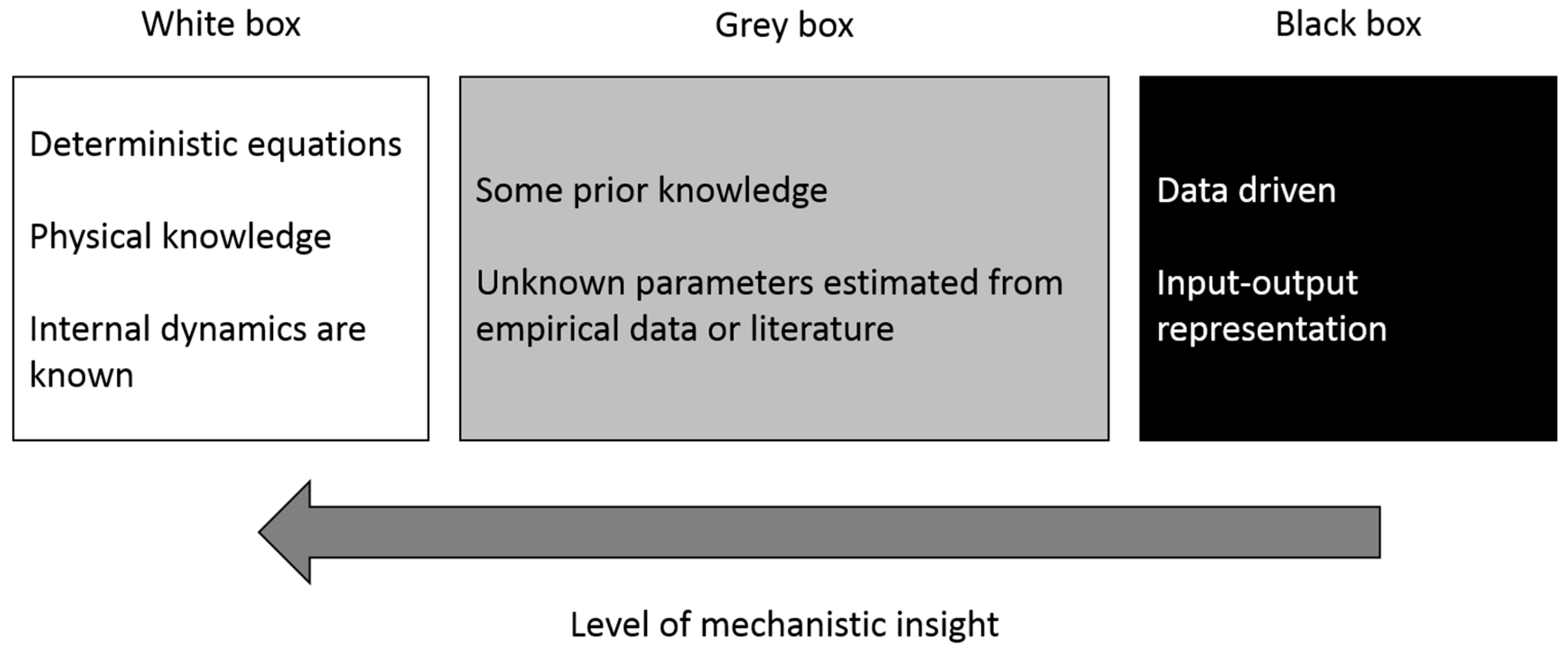
It is common for modellers to classify models into three categories:

• White box;
• Grey box;
• Black box.

White box, or transparent, models are purely theoretical, whereas black box models assume no model structure and are data driven. That is to say, black box models are selected to fit one or more particular data sets without reference to the processes at work. The widely used statistical linear and polynomial regression models are examples of black box models. Grey box models, such as ECMs, combine partial theoretical structure with data to complete the model [17,18], as illustrated in Figure 1.

In order to make the models as accurate as possible, it is preferable to use a priori information to assign numerical values to the parameters. However, as is often the case in modelling complex systems, ECMs contain unknown parameters. For example, it is known that the internal impedance of LIBs varies with temperature and SOC, but the precise relationship is not defined. These parameters are estimated from experimental data using statistical methods (i.e., system identification). How accurately and robustly these unknown parameters can be estimated from characterisation data is of utmost importance to modellers and, ultimately, the BMS. It is therefore essential to determine whether these parameters can be uniquely identified from the proposed experiments to gather experimental data.

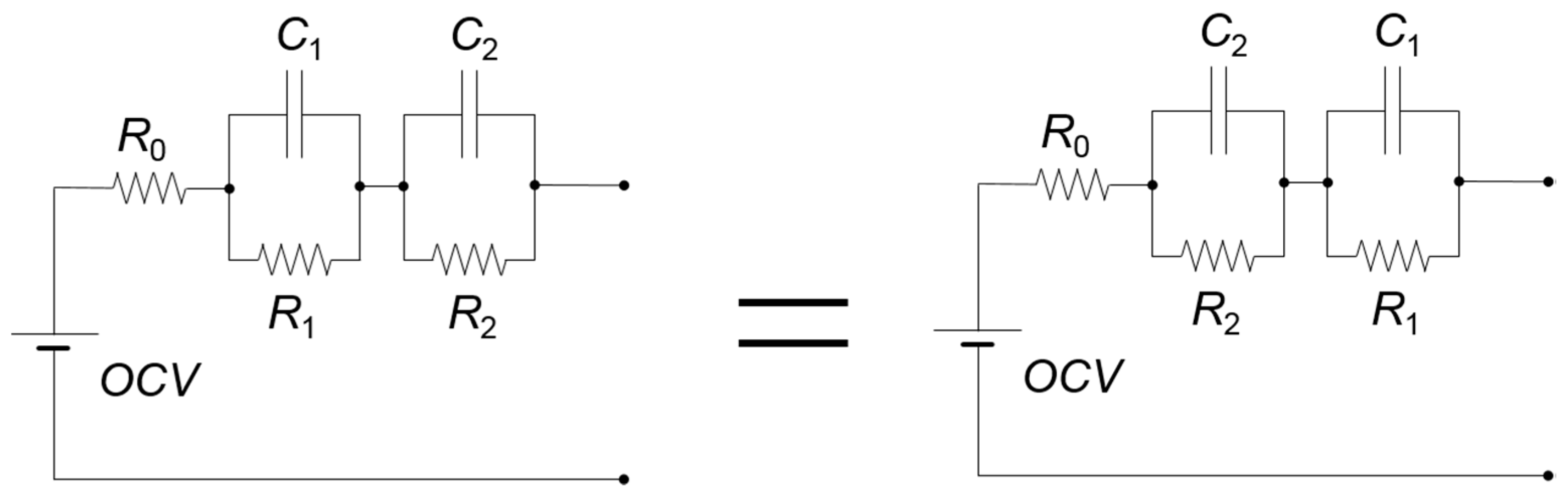
A typical ECM often used in LIB modelling is the second-order resistor–capacitor (RC) network. Swapping the RC pairs of this model, as illustrated in Figure 2, does not affect the output because this model has two possible parameter sets that are interchangeable. It is generally accepted that the midfrequency RC pair (e.g., R₁C₁) represents the faradic charge transfer resistance and its relative double layer capacitance at the electrode/electrolyte interface, and the high-frequency pair (e.g., R₂C₂) represents the solid-state interface layer on the active electrode material [19,20,21]. However, without this additional information about the relative size of the RC pairs, it would not be possible to assign physical phenomena to a two-RC network. During usage, LIBs degrade, and key characteristics such as impedance increase due to ageing mechanisms (e.g., solid electrolyte interphase (SEI) layer growth) [22,23,24]. It is desired for the BMS to monitor these alterations to battery dynamics. It is therefore very difficult to track the evolution of each RC pair if they can switch for every estimation.

Unidentifiable parameters (i.e., parameters that cannot be uniquely identified) can take an infinite number of numerical values, rendering any numerical estimate obtained from parameter estimation meaningless. Despite the implications, LIB models containing in excess of 19 resistors and 30 capacitors can be found in the literature with no consideration for structural identifiability [25]. In this ECM, diffusion and migration were represented by a complex ladder network. Assigning numerical values to unidentifiable parameters—which represent real physical or chemical processes—is meaningless and nullifies the mechanistic properties of the model. Techniques for structural identifiability analysis determine whether unknown model parameters have unique values given the available observation(s) [26].

The aim of this paper is to highlight the critical aspects of structural identifiability, with emphasis on application in LIB modelling. Twelve ECMs covering the majority of model templates used previously are examined in detail to illustrate the importance of structural identifiability prior to performing experiments for parameter estimation. The methods used are applicable for all LIB chemistries and formats that are described by ECMs.

The remainder of this article is laid out as follows. Section 2 defines the concept of structural identifiability and Section 3 describes the 12 models that have been investigated. Details of the methods implemented to ascertain the aforementioned models’ structural identifiability analyses, including a worked example, are found in Section 4. The results are summarised in Section 5, and these are discussed in Section 6. Finally, Section 7 contains the conclusions drawn.

2. Structural Identifiability

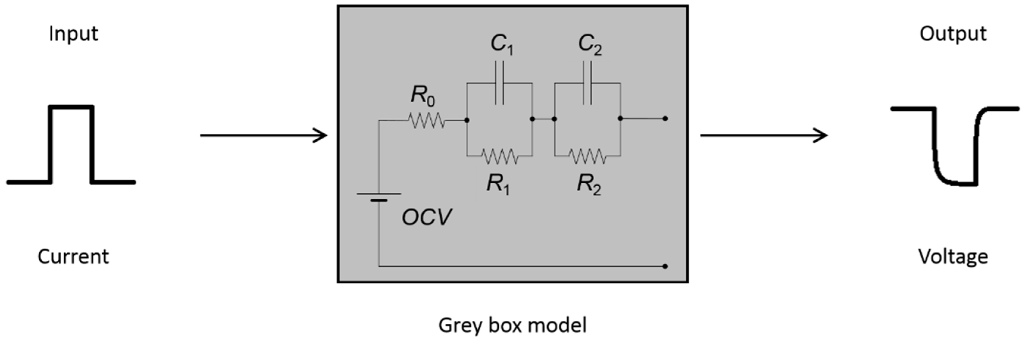
Figure 3 illustrates a typical ECM implementation. A current input signal into the ECM produces a corresponding voltage output signal, where discharge current is positive as per automotive testing standards [27].

Given a model circuit diagram, it is possible to describe mathematically the exact relationship between the input and the output of the model. As this relationship depends on the model structure (i.e., the circuit diagram), it is simply referred to as the input/output structure. As discussed previously, there are unknown model parameters in this relationship that need to be estimated from empirical data. Given an input/output structure and some proposed experiments to collect data for parameter estimation, structural identifiability analysis considers the uniqueness of the unknown model parameters. It is a purely theoretical method that assumes the data is perfect and noise-free [28,29]. This is an important, but often overlooked, theoretical prerequisite to experiment design, system identification, and parameter estimation, since numerical estimates for unidentifiable parameters are effectively meaningless; unidentifiable parameters have an infinite number of possible numerical solutions. If parameter estimates are to be used to inform about charging and discharging strategies, or other critical decisions, then it is essential that the parameters be uniquely identifiable. Parameter-fitting software packages generally struggle when attempting to estimate nonidentifiable parameters; numerical optimisation algorithms may oscillate between numerous possible solutions, considerably reducing the confidence in the accuracy of the parameter values.

Observation and measurement errors are not included in the a priori theoretical analysis. Structural identifiability is concerned with establishing whether or not there is enough information in the observations to uniquely determine the unknown parameters. Structural identifiability assumes continuous, noise-free data, therefore, it is not necessary to physically perform the experiments; the results can be established from the model structure and experiment design, which generally has implications on which data should be collected and how. The issue of trying to estimate parameter values in the presence of real, often discontinuous, and noisy data is a nonstructural quantitative problem. It only necessitates a very small amount of a posteriori kinetic data to solve the problem [30]. The a posteriori numerical identifiability analyses are based on local sensitivities of the unknown parameters, the Fisher information matrix, the covariance matrix, or the Hessian of the least square function [31]. It is a separate technical problem that the modeller needs to address, and it should not detract from the prerequisite of satisfying a priori structural identifiability. It is important to note that an a priori structurally identifiable model does not necessarily guarantee a posteriori numerical parameter identifiability, for example [32]. However, it does greatly increase the confidence in the parameter estimation process for the given system observation(s). A posteriori numerical parameter identifiability cannot be guaranteed, as it is dependent on the quality of the data (e.g., sampling rate, noise, measurement error).

For a given output, an unidentifiable parameter can take an (unaccountably) infinite set of values, whereas a non-uniquely (locally) identifiable parameter can take any of a distinct (countable) set of values. A parameter is globally identifiable if, for a given output, it can only take one value.

If all of the unknown parameters are globally identifiable, the system model is structurally globally identifiable (SGI). In the case where at least one parameter is locally identifiable and all the remaining parameters, if any, are globally identifiable, then the model is structurally locally identifiable (SLI). In the case where at least one parameter is unidentifiable, then the model is structurally unidentifiable (SU).

Although an essential prerequisite for experiment design, system identification, and parameter estimation, structural identifiability of Li-ion battery models has been mostly overlooked until recently [33,34,35]. Sitterly et al. [33] ascertained that the resistance–capacitance battery model developed at the National Renewable Energy Laboratory (NREL) [36] as part of advanced vehicle simulator (ADVISOR) [37] is SU by demonstrating that the number of unknown parameters exceeds the number coefficients of the resulting transfer function of the model. Sitterly et al. [33] reduces the number of unknown parameters in order to ensure the reduced model is globally structurally identifiable when only the terminal voltage and current are measured.

Rausch et al. [34] have attempted to investigate the structural identifiability of a first-order RC model by considering the observability of the unknown parameters. The observability analyses are not rigorous, and observability has been shown to be insufficient to guarantee structural identifiability [38]. Rausch et al. [34] also consider two Li-ion cells in parallel and conclude that the internal parameters are observable and therefore extractable. It can be shown that two first-order RC models in parallel with only one current and voltage sensor is in fact SLI. Alavi et al. [35] have endeavoured to investigate the structural identifiability of a modified version of the Randles circuit [39]. The analysis also lacks rigour, and structural identifiability is confused with numerical identifiability.

While structural identifiability of battery models has recently attracted interest, only linear ECMs have been investigated thus far. Numerous techniques for performing a structural identifiability analysis on linear parametric models exist, and this is a well-understood topic [28,29,40]. The Laplace transform approach, or transfer function approach, is normally the method selected to analyse linear models; see [26] for a thorough discussion of this method. However, some ECMs that contain hysteresis are nonlinear, and the Laplace transform approach is not applicable to nonlinear systems. Hu et al. [41] present a comparative study of 12 linear and nonlinear ECMs in 2012, including hysteresis, for LIBs; these 12 models are systematically analysed in order to establish whether they are structurally identifiable and hence useful in a BMS application. It is essential for ECMs to be globally structurally identifiable in order for ECM parameters to be physically meaningful.

3. Models

Hu et al. [41] presented a comparative study of 12 linear and nonlinear ECMs for LIBs in 2012, which were selected from state-of-the-art lumped models reported in the literature. The models were selected to represent a comprehensive subset covering the majority of model templates used previously. Data sets collected for two cell chemistries (LiNiMnCoO₂) and LiFePO₄) at three different temperatures (10 °C, 22 °C, and 35 °C) were used for characterisation. The models are summarised in

Table 1. Twelve ECM model equations.

Model	Equations
1. The combined model	$$V(t)=k_0-\frac{k_1}{z(t)}-k_{2}z(t)+k_3\ln \left(z(t)\right)+k_4\ln \left(1-z(t)\right)-R_{0}I(t)$$ (1) $$\frac{dz(t)}{dt}=-\frac{{\mathsf{\eta }}_{i}I(t)}{C_n}$$ (2) where V(t), z(t) and I(t) are the battery terminal voltage, state of charge (SOC), and current, respectively. The unknown parameter vector $\mathsf{\theta }=\left[k_0,k_1,k_2,k_3,k_4,R_0^{+},R_0^{-}\right]$, where $R_0^{+}$ and $R_0^{-}$ are internal resistances for the discharge and charge, respectively.
2. The simple model	$$V(t)=OCV-R_{0}I(t),\mathsf{\theta }=\left[OC{V}_1,\dots ,OC{V}_{12},R_0^{+},R_0^{-}\right]$$ (3)
3. The zero-state hysteresis model	$$V(t)=OCV-R_{0}I(t)-s_{k}M,s_k=\{\begin{array}{c}1,\\ -1,\\ s_{k-1},\end{array}\begin{array}{c}I(t)>\mathsf{\epsilon }\\ I(t)<-\mathsf{\epsilon }\\ \left|I(t)\right|\le \mathsf{\epsilon }\end{array}$$ (4) where M is assumed to be a constant coefficient depicting the hysteresis level and ε is adequately small and positive. $\mathsf{\theta }=\left[OC{V}_1,\dots ,OC{V}_{12},R_0^{+},R_0^{-},M\right]$.
4. The one-state hysteresis model	$$V(t)=OCV-R_{0}I(t)+h(t)$$ (5) $$\frac{dh(t)}{dt}=\left(H-h(t)\right)\mathsf{\kappa }i(t),\mathsf{\theta }=\left[OC{V}_1,\dots ,OC{V}_{12},R_0^{+},R_0^{-},\mathsf{\kappa },H^{+},H^{-}\right]$$ (6) where h(t) is the hysteresis voltage, κ is a decaying factor, and H+ and H− are the maximum amount of hysteresis for discharge (negative) and charge (positive), respectively.
5. The enhanced self-correcting model (two-state low-pass filter)	$$V(t)=OCV-R_{0}I(t)+h(t)+g_1{f}_1+g_2{f}_2$$ (7)
6. The enhanced self-correcting model (four-state low-pass filter)	$$V(t)=OCV-R_{0}I(t)+h(t)+g_1{f}_1+g_2{f}_2+g_3{f}_3+g_4{f}_4$$ (8)
7. The first-order RC model	$$V(t)=OCV-R_0{I}_L(t)-R_1{I}_1(t)$$ (9) $$\frac{d{I}_1(t)}{dt}=\frac{I(t)-I_1(t)}{{\mathsf{\tau }}_1}$$ (10)
8. The first-order RC model with hysteresis	$$V(t)=OCV+h(t)-R_0{I}_L(t)-R_1{I}_1(t)$$ (11)
9. The second-order RC model	$$V(t)=OCV-R_0{I}_L(t)-R_1{I}_1(t)-R_2{I}_2(t)$$ (12) $$\frac{d{I}_n(t)}{dt}=\frac{I(t)-I_n(t)}{{\mathsf{\tau }}_n}$$ (13)
10. The second-order RC model with hysteresis	$$V(t)=OCV-R_0{I}_L(t)-R_1{I}_1(t)-R_2{I}_2(t)$$ (14)
11. The third-order RC model	$$V(t)=OCV-R_0{I}_L(t)-R_1{I}_1(t)-R_2{I}_2(t)-R_3{I}_3(t)$$ (15)
12. The third-order RC model with hysteresis	$$V(t)=OCV+h(t)-R_0{I}_L(t)-R_1{I}_1(t)-R_2{I}_2(t)-R_3{I}_3(t)$$ (16)

.

Apart from Model 1, all the models use a look-up table with 12 entries to calculate open-circuit voltage (OCV). These and the remaining model parameters to be estimated from experimental data are summarised in Table 1. In the study [41], the models are discretised for optimisation and implementation; however, in this paper, the models are described and analysed in continuous form (a requirement for structural identifiability analyses). The issue of trying to estimate parameter values from discretised models is a nonstructural quantitative problem. For the purpose of the analyses, it is assumed that the input current and the corresponding output voltage are known (measured).

4. Methodology

Numerous techniques for performing a structural identifiability analysis on linear parametric models exist, and this is a well-understood topic [28,29,40]. In comparison, assessing structural identifiability of nonlinear dynamic systems is particularly challenging [42,43]. Although there are a number of techniques available for nonlinear systems, many of these approaches rapidly become mathematically intractable with increasing model size and complexity [44,45]. Significant computational problems can arise for these, even for relatively simple models [46,47].

There is no “one size fits all” technique that is amenable to every model; all the methods have varying levels of success, depending on the model to which they are applied. Furthermore, it is virtually impossible to predict which methods are guaranteed to work for a specific model structure. Selecting an appropriate approach is problematic and they are often difficult to implement.

In this paper, three methods are utilised: the Taylor series approach [48], the characteristic set differential algebra approach [49,50], and the algebraic input/output relationship approach [51]. All three approaches are selected for each of the 12 ECMs; depending on the model structure, and the applicability and suitability of each technique, the relevant approaches are implemented for each of the 12 ECMS.

Due to the complex nature (see worked example in Section 4.3 below) of the analytical approaches for the nonlinear models, a symbolic computational package, namely Maplesoft Maple 2010 [52], was used to perform the analyses. Other packages are suitable, such as Wolfram Research Mathematica 2015 [53].

4.1. Taylor Series Expansion

This general method, introduced by Pohjanpalo in 1978 [48], is commonly used for systems with a single input and can be applied to both linear and nonlinear systems. Given a nonlinear mathematical model of the following general form:

$$\dot{\mathit{x}}(t,\mathit{p})=\mathit{f}(\mathit{x}(t,\mathit{p}),\mathit{p})$$

(17)

$$\mathit{x}(0,\mathit{p})={\mathit{x}}_0(\mathit{p})$$

(18)

$$\mathit{y}(t,\mathit{p})=\mathit{h}(\mathit{x}(t,\mathit{p}),\mathit{p})$$

(19)

where p is the r dimensional vector of unknown parameters. The n dimensional vector $\mathit{x}(t,\mathit{p})$ is the state vector, such that $x_0(\mathit{p})$ is the initial state and $\mathit{y}(t,\mathit{p})$ is the observation vector. The components of the observation vector $y_i(t,\mathit{p})$ are expanded as a Taylor series around the known initial condition:

$$y_i(t,\mathit{p})=y_i(0,\mathit{p})+{\dot{y}}_i(0,\mathit{p})t+{\ddot{y}}_i(0,\mathit{p})\frac{t^2}{2!}+\dots +y_i^{\left(k\right)}(0,\mathit{p})\frac{t^k}{k!}+\dots$$

(20)

where:

$$y_i^{\left(k\right)}(0,\mathit{p})={\frac{d^k{y}_i}{d{t}^k}|}_{t=0}$$

(21)

The Taylor series coefficients $y_i^{(k)}(t,\mathit{p})$ are measurable and unique for a particular output. Equating the Taylor series coefficients obtained from $\mathit{y}(t,\mathit{p})$ with those derived from $\mathit{y}(t,\tilde{\mathit{p}})$produces a system of equations. If there is only one solution for the unknown parameters, then the model is SGI. The total number of unknown model parameters determines the minimum number of Taylor series coefficients required to establish structural identifiability, and this causes significant computational problems in models with numerous unknown model parameters.

4.2. Differential Algebra Approach Using Characteristic Sets

This approach consists of generating the input/output structure of the given model of the general form (17)–(19) solely in terms of the observation function $\mathit{y}(t,\mathit{p})$ and its derivatives using characteristic sets [49,50]. Assuming the observation $\mathit{y}(t,\mathit{p})=\mathit{h}(\mathit{x}(t,\mathit{p}),\mathit{p})$ is linear, this approach considers two parameter vectors, $\mathit{p}$ and $\tilde{\mathit{p}}$, that produce the same output for all $t$, and thus produce the same derivatives of the observation for all $t$, that is:

$$y^{(n)}(t,\mathit{p})=y^{(n)}(t,\tilde{\mathit{p}}),\mathrm{for}\mathrm{a11}t$$

(22)

If it is possible to generate an expression $g(y,\dots ,y^{(n-1)},\mathit{p})$ derived from the model equations $\mathit{f}(\mathit{x}(t,\mathit{p}),\mathit{p})$ purely in terms of the observation vector $\mathit{y}(t,\mathit{p})$ and its derivatives, then the approach entails solving:

$$g(y,\dots ,y^{\left(n-1\right)},\mathit{p})=g(y,\dots ,y^{(n-1)},\tilde{\mathit{p}})$$

(23)

for $\mathit{p}$. This approach initially entails establishing an observability rank criterion (ORC). This is performed by defining a function H given by:

$$\mathit{H}(x,\mathit{p})={({\mathsf{\mu }}_1(x,\mathit{p}),\dots ,{\mathsf{\mu }}_n(t,\mathit{p}))}^T$$

(24)

where ${\mathsf{\mu }}_1(\mathit{x},\mathit{p})$ is the observation function $\mathit{h}$ from Equation (19), and ${\mathsf{\mu }}_n(\mathit{x},\mathit{p})$ is the Lie derivative of the previous term, given by:

$${\mathsf{\mu }}_n(x,\mathit{p})=L_f{\mathsf{\mu }}_{n-1}(x)=\frac{\partial {\mathsf{\mu }}_{n-1}}{\partial \mathit{x}}(x)\cdot \mathit{f}(x)$$

(25)

and $\mathit{f}$, the vector of the system coordinate functions given by Equation (17). If the Jacobian matrix with respect to x, evaluated at ${\mathit{x}}_0(\mathit{p})$, of the resultant function $\mathit{H}(\cdot ,\mathit{p})$ is non-singular, then the system of Equations (17)–(19) is said to satisfy the ORC and it is possible to construct a smooth mapping from the state corresponding to a parameter vector $\tilde{\mathit{p}}$, indistinguishable from $\mathit{p}$, to the state corresponding to $\mathit{p}$. This approach is implemented using the Rosenfeld–Gröbner algorithm in Maple 2010, which calculates a characteristic set for the model with a particular ranking of variables, where one member of the characteristic set gives the input/output map $g(y,\dots ,y^{(n-1)},\mathit{p})$. A second input/output map is generated by substituting $\mathit{p}$ for $\tilde{\mathit{p}}$ in the original map. If equating the monomials of these two functions produces only one solution for the unknown parameters, then the system is SGI. The Rosenfeld–Gröbner algorithm in Maple 2010 can be very memory-intensive, particularly if the model equations contain complicated nonlinear terms. See [54] for examples of where this approach fails to yield results for nonlinear models, as there is not enough memory available for Maple 2010 to perform the required symbolic calculations.

4.3. Algebraic Input/Output Relationship Approach

This is the most recent approach, developed by Evans et al. in 2012 [51]. Given a model of the general form (17)–(19) that satisfies the ORC, this approach generates the corresponding input/output map for the system. This approach requires calculating the Lie derivatives of the observation function, defined in Equation (25). These are used as inputs into the univariate polynomial or Groebner bases algorithms in Maple, producing the input/output relationship for the model. Again, a second input/output map is generated by substituting $\mathit{p}$ for $\tilde{\mathit{p}}$ in the original input/output relationship. If equating the monomials of these functions produces only one solution for the unknown parameters, then the system is SGI. In terms of run time and memory utilisation, the univariate polynomial algorithm in Maple 2010 is the most efficient algorithm out of all the approaches described [54]. However, it can still be very memory-intensive, particularly if the model equations contain complicated nonlinear terms [54] (see Section 2).

Model 8, the first-order model with hysteresis, is the most commonly used ECM and is selected as a worked exampled to detail this approach.

Model 8—First-Order Model with Hysteresis Worked Example

The model equations are restated below for clarity:

$$V(t)=OCV(z)+h(t)-R_0{I}_L(t)-R_1{I}_1(t)$$

(26)

$$\frac{d{I}_1(t)}{dt}=\frac{I_L(t)-I_1(t)}{{\mathsf{\tau }}_1}$$

(27)

$$\frac{dh(t)}{dt}=\left(H-h(t)\right)\mathsf{\kappa }{I}_L(t)$$

(28)

where V(t) is the battery terminal voltage, z(t) is the SOC, I_L(t) is the current, h(t) is the hysteresis voltage, $\mathsf{\kappa }$ is a decaying factor, and H⁺ and H⁻ are the maximum amount of hysteresis for discharge (negative) and charge (positive), respectively. $R_0^{+}$ and $R_0^{-}$ are internal resistances for the discharge and charge, respectively. OCV(z) represents the open-circuit voltage, which is a function of SOC. In the study [41], this is implemented by a look-up table with 12 entries, however, there is no information regarding how OCV(z) is interpolated between values. In this paper, it is assumed that linear interpolation is implemented, that is:

$$OCV(z)=mz(t)+p$$

(29)

where m is an unknown constant and p is a known constant. p is known, as it is assumed that the initial conditions are known. It is assumed that the data sets for parameter estimation are split into 11 subsets according to the 12 SOC thresholds. There is no information in the study [41] as to the values of the thresholds, however, this is not important for structural identifiability analysis. Here, we look at one subset and therefore one value of m. If one subset is structurally identifiable, then by symmetry they are all structurally identifiable. SOC is defined as:

$$\frac{dz(t)}{dt}=-\frac{\mathsf{\eta }{I}_L(t)}{C}$$

(30)

where η is an efficiency constant and C is the nominal capacity. As these are not in the optimisation variable vector the study [41], it is assumed that these constants are known. The unknown parameter vector is $\mathsf{\theta }=\left[m,R_0,\mathsf{\kappa },H,R_1,{\mathsf{\tau }}_1\right]$, the input vector is:

$$u(t,\mathsf{\theta })=I_L(t)$$

(31)

and the observation vector is:

$$y(t,\mathsf{\theta })=V(t)$$

(32)

Switching from H⁺ to H⁻ and from $R_0^{+}$ to $R_0^{-}$ introduces discontinuities in the model. These cause complications for the structural identifiability analyses, as all the methods described require the observation to be smooth and continuous so that it is differentiable. In order to perform the analyses, a continuous case is considered (i.e., a pure discharge scenario). If the discharge model is structurally identifiable, then the charge model is structurally identifiable by symmetry.

The first three Lie derivatives are calculated using (25):

$${\mathsf{\mu }}_1=y=mz+p+h-R_{0}u-R_1{I}_1$$

(33)

$${\mathsf{\mu }}_2=\mathsf{\kappa }u\left(H-h\right)-R_0{u}^{(1)}-\frac{\mathsf{\eta }mu}{C}+\frac{R_1\left(I_1-u\right)}{{\mathsf{\tau }}_1}$$

(34)

$${\mathsf{\mu }}_3=-\left(H-h\right){\mathsf{\kappa }}^2{u}^2+\left(H-h\right)\mathsf{\kappa }{u}^{(1)}-R_0{u}^{(2)}-\frac{\mathsf{\eta }m{u}^{(1)}}{C}-\frac{R_1{u}^{(1)}}{{\mathsf{\tau }}_1}+\frac{R_1\left(I_1-u^{(1)}\right)}{{\mathsf{\tau }}_1^2}$$

(35)

where:

$$u^{(n)}=\frac{d^{n}u(t)}{d{t}^n}$$

(36)

The Jacobian matrix with respect to $\mathit{x}=\left[I_1,h,z\right]$, evaluated at $\mathit{x}(0)$, of the resultant function H defined in (24), is given by:

$$\left[\begin{array}{ccc}-R_1& 1& m\\ \frac{R_1}{{\mathsf{\tau }}_1}& -\mathsf{\kappa }u& 0\\ \frac{-R_1}{{\mathsf{\tau }}_1^2}& {\mathsf{\kappa }}^2{u}^2-\mathsf{\kappa }{u}^{(1)}& 0\end{array}\right]$$

(37)

which is non-singular if u or u⁽¹⁾ is non-zero. The model satisfies the ORC as long as the initial input current or the first derivative of the initial input current is not equal to zero. The univariate polynomial algorithm in Maple 2010 is used to calculate the input/output map:

$$\begin{array}{c}{y}^{(3)}=-\frac{1}{C{\mathsf{\tau }}_1\left({\mathsf{\tau }}_1{u}^{(1)}-{\mathsf{\kappa }\mathsf{\tau }}_1{u}^2+u\right)}[-{\mathsf{\eta }\mathsf{\kappa }}^{2}m{\mathsf{\tau }}_1{u}^4-{\mathsf{\kappa }}^2{\mathsf{\tau }}_1\left(\mathsf{\eta }m{\mathsf{\tau }}_1+C{R}_0+C{R}_1\right)u^3{u}^{(1)}-C{R}_0{\mathsf{\kappa }}^2{\mathsf{\tau }}_1^2{u}^3{u}^{(2)}\hfill \\ -C{\mathsf{\kappa }}^2{\mathsf{\tau }}_1{u}^3{y}^{(1)}-C{\mathsf{\kappa }}^2{\mathsf{\tau }}_1^2{u}^3{y}^{(2)}+\mathsf{\eta }\mathsf{\kappa }m{u}^3+C\mathsf{\kappa }{u}^2{y}^{(1)}+\mathsf{\kappa }\left(3\mathsf{\eta }m{\mathsf{\tau }}_1+C{R}_0+C{R}_1\right)u^2{u}^{(1)}-C{\mathsf{\tau }}_1{u}^{(2)}{y}^{(1)}\hfill \\ +3{\mathsf{\kappa }\mathsf{\tau }}_1\left({\mathsf{\eta }\mathsf{\tau }}_1+C{R}_0+C{R}_1\right)u{u}^{(1)}{u}^2+3C{R}_0{\mathsf{\kappa }\mathsf{\tau }}_1^{2}u{u}^{(1)}{u}^{(2)}+3C{\mathsf{\kappa }\mathsf{\tau }}_{1}u{u}^{(1)}{y}^{(1)}-C{R}_0{\mathsf{\kappa }\mathsf{\tau }}_1^2{u}^2{u}^{(3)}\hfill \\ +3C{\mathsf{\kappa }\mathsf{\tau }}_1^{2}u{u}^{(1)}{y}^{(2)}+C\left(R_0+R_1\right)u{u}^{(2)}+C{R}_0{\mathsf{\tau }}_{1}u{u}^{(3)}+Cu\text{}{y}^{(2)}-C{\mathsf{\tau }}_1^2{u}^{(2)}{y}^{(2)}-C{u}^{(1)}{y}^{(1)}\hfill \\ -C\left(R_0+R_1\right)u^{{(1)}_2}-C{R}_0{\mathsf{\tau }}_1{u}^{(1)}{u}^{(2)}+C{R}_0{\mathsf{\tau }}_1^2{u}^{(1)}{u}^{(3)}-C{R}_0{\mathsf{\tau }}_1^2{u}^{{(2)}_2}-{\mathsf{\kappa }\mathsf{\tau }}_1\left({\mathsf{\eta }\mathsf{\tau }}_1+C{R}_1\right)u^2{u}^{(2)}]\hfill \end{array}$$

(38)

where:

$$y^{(n)}=\frac{d^{n}y(t)}{d{t}^n}$$

(39)

This input/output structure of the model is solely in terms of the measured input and output variables $\left[y,u\right]$ and their derivatives $\left[y^{(1)},y^{(2)},y^{(3)},u^{(1)},u^{(2)},u^{(3)}\right]$. A second input/output map is generated by substituting $\mathsf{\theta }$ and $\tilde{\mathsf{\theta }}$ in the original map. Equating the monomials of these two functions and solving for the unknown parameters produces the following solution:

$$\left[\tilde{m}=m,{\tilde{R}}_0=R_0,\tilde{\mathsf{\kappa }}=\mathsf{\kappa },\tilde{H}=\tilde{H},{\tilde{R}}_1=R_1,{\tilde{\mathsf{\tau }}}_1={\mathsf{\tau }}_1\right]$$

(40)

This solution is not unique, as H can take any value. Most of the unknown parameters $\left[m,R_0,\mathsf{\kappa },R_1,{\mathsf{\tau }}_1\right]$ are uniquely identifiable, however, H is unidentifiable. The latter is expected, as H is not found in the input/output map. The input/output structure does not consider the system’s initial conditions. This can be done by evaluating the Lie derivatives at the initial conditions:

$${\mathsf{\mu }}_1=m{z}_0(0)+p+h(0)-R_{0}u-R_1{I}_1(0)$$

(41)

$${\mathsf{\mu }}_2=\mathsf{\kappa }u\left(H-h(0)\right)-R_0{u}^{(1)}-\frac{\mathsf{\eta }mu}{C}+\frac{R_1\left(I_1(0)-u\right)}{{\mathsf{\tau }}_1}$$

(42)

$${\mathsf{\mu }}_3=-\left(H-h(0)\right){\mathsf{\kappa }}^2{u}^2+\left(H-h(0)\right)\mathsf{\kappa }{u}^{(1)}-R_0{u}^{(2)}-\frac{\mathsf{\eta }m{u}^{(1)}}{C}-\frac{R_1{u}^{(1)}}{{\mathsf{\tau }}_1}+\frac{R_1\left(I_1(0)-u^{(1)}\right)}{{\mathsf{\tau }}_1^2}$$

(43)

The input, u, and its derivatives, u⁽¹⁾ and u⁽²⁾, are evaluated at t = 0. Since the input is arbitrary and free for choice, the input, u, and its derivatives, u⁽¹⁾ and u⁽²⁾, can be treated as indeterminates. It can be shown from Equation (42) that H is identifiable if all the initial conditions are known (i.e., z₀(0), h(0), and I₁(0)).

The unknown model parameters are therefore structurally identifiable. However, only a continuous case was considered (i.e., a pure discharge scenario). As discussed previously, the charge model is also structurally identifiable by symmetry. However, these models are only globally structurally identifiable if the initial conditions are known. During a mixed scenario, when the model switches (e.g., from charge to discharge), some of the initial conditions (i.e., h(0) and I₁(0)) are unknown, and therefore H cannot be uniquely determined. Consequently, Model 8 is SU.

5. Results

Model 1 was analysed using the Taylor series method, as all the other approaches cannot be utilised on models with non-polynomial terms such as logarithms. The remaining models were analysed using all three approaches. In all instances, both the differential algebra approach, using characteristic sets, and algebraic input/output relationship approach methods yield the same input/output structures and, therefore, identical results. The Taylor series expansion method confirms the results obtained. The outcomes of the structurally identifiability analyses for the 12 models are summarised in

Table 2. Structural identifiability analyses results.

Model	Identifiable Parameters	Unidentifiable Parameters	Identifiability Result
1. The combined model	$\left\{k_0,k_1,k_2,k_3,k_4,R_0\right\}$	-	SGI
2. The simple model	$\left\{m,p,R_0\right\}$	-	SGI
3. The zero-state hysteresis model	$\left\{m,R_0\right\}$	$\left\{p,M\right\}$	SU
4. The one-state hysteresis model	$\left\{m,R_0,\mathsf{\kappa }\right\}$	$\left\{p,H\right\}$	SU
5. The enhanced self-correcting model (two-state low-pass filter)	$\left\{m,R_0,\mathsf{\kappa }\right\}$	$\left\{p,H,g_1,{\mathsf{\alpha }}_1,g_2,{\mathsf{\alpha }}_2\right\}$	SU
6. The enhanced self-correcting model (four-state low-pass filter)	$\left\{m,R_0,\mathsf{\kappa }\right\}$	$\left\{p,H,g_{1-4},{\mathsf{\alpha }}_{1-4}\right\}$	SU
7. The first-order RC model	$\left\{m,p,R_0,R_1,{\mathsf{\tau }}_1\right\}$	-	SGI
8. The first-order RC model with hysteresis	$\left\{m,R_0,R_1,{\mathsf{\tau }}_1\right\}$	$\left\{p,H\right\}$	SU
9. The second-order RC model	$\left\{m,p,R_0\right\}$	$\left\{R_1,{\mathsf{\tau }}_1\right\}\iff \left\{R_2,{\mathsf{\tau }}_2\right\}$	SLI
10. The second-order RC model with hysteresis	$\left\{m,R_0,\mathsf{\kappa }\right\}$	$\left\{p,H\right\}$, $\left\{R_1,{\mathsf{\tau }}_1\right\}\iff \left\{R_2,{\mathsf{\tau }}_2\right\}$	SU
11. The third-order RC model	$\left\{m,p,R_0\right\}$	$\left\{R_1,{\mathsf{\tau }}_1\right\}\iff \left\{R_2,{\mathsf{\tau }}_2\right\}\iff \left\{R_3,{\mathsf{\tau }}_3\right\}$	SLI
12. The third-order RC model with hysteresis	$\left\{m,R_0,\mathsf{\kappa }\right\}$	$\left\{p,H\right\}$, $\left\{R_1,{\mathsf{\tau }}_1\right\}\iff \left\{R_2,{\mathsf{\tau }}_2\right\}\iff \left\{R_3,{\mathsf{\tau }}_3\right\}$	SU

below.

For Model 1, the Taylor series expansion analysis reveals that k₀ is only globally identifiable for known initial conditions. Although some of the initial conditions (i.e., h(0) and I₁(0)) are unknown when the model switches (e.g., from charge to discharge), k₀ is simply an offset, which can be easily estimated from one initial condition value, so the model is SGI.

The input/output structures for Models 2 and 7 reveal that p is only globally identifiable for known initial conditions. As above, p is also simply an offset, which can be easily estimated from one initial condition value, and the models are SGI.

On the other hand, the input/output structures for Model 3 demonstrate that p and M are unidentifiable, even with known initial conditions. Model 3 is therefore SU.

Similarly, the input/output structures for Models 4, 8, 10, and 12 show that p and H are unidentifiable, even with known initial conditions. As a result, Models 4, 8, 10, and 12 are also SU.

Models 5 and 6 are challenging to analyse, as both are discrete models and equivalent continuous models need to be derived in order to perform the analyses. However, both models share the same structure for OCV and hysteresis, which have been shown in the previous analyses (Models 4, 8, 10, and 12) to be indistinguishable. Consequently, p and H are also unidentifiable in Models 5 and 6. It follows that the additional terms are also unidentifiable. Although this has not been demonstrated explicitly, in the unlikely case that those terms would be identifiable, the model would still remain unidentifiable, as two parameters cannot be distinguished.

Finally, the input/output structures for Models 9 and 11 show that the RC pairs are indistinguishable. Model 9 has two possible solutions:

$$\left\{m=\tilde{m},p=\tilde{p},R_0={\tilde{R}}_0,R_1={\tilde{R}}_1,{\mathsf{\tau }}_1={\tilde{\mathsf{\tau }}}_1,R_2={\tilde{R}}_2,{\mathsf{\tau }}_2={\tilde{\mathsf{\tau }}}_2\right\}$$

(44)

and:

$$\left\{m=\tilde{m},p=\tilde{p},R_0={\tilde{R}}_0,R_1={\tilde{R}}_2,{\mathsf{\tau }}_1={\tilde{\mathsf{\tau }}}_2,R_2={\tilde{R}}_1,{\mathsf{\tau }}_2={\tilde{\mathsf{\tau }}}_1\right\}$$

(45)

The first three parameters—m, p, and R₀—are globally identifiable, however, R₁ and τ₁ are interchangeable with R₂ and τ₂ pairwise. Similarly, Model 11 has six distinct solutions and there are three RC pairs and six different possible combinations.

6. Discussion

Only the simplest models—Models 1, 2, and 7—are SGI. However, it is important to note that for those models, k₀ and p are only identifiable from the initial conditions. This will affect the accuracy of the numerical values assigned in the parameter estimation. Most parameters are estimated from time series data, whereas k₀ and p can only be uniquely identified from the initial conditions. It is recommended to perform the parameter estimation over a range of different initial conditions in order to accurately estimate those parameters, as they will be dependent on initial condition accuracy.

The higher-order RC network without hysteresis—Models 9 and 11—are locally identifiable, as the RC pairs are interchangeable, an intuitive result discussed in Section 1, as the RC pairs can be swapped in the circuit diagram without altering the model structure. SLI models may cause parameter estimation algorithms to oscillate between the distinct solutions. It is recommended to add additional constraints to the model for the parameter estimation (e.g., using upper and lower bounds for these parameters or defining the relationship with regard to the relative size of the local parameters). It is generally accepted that the midfrequency RC pair represents the faradic charge transfer resistance and its relative double-layer capacitance at the electrode/electrolyte interface, and the high-frequency pair represents the solid-state interface layer on the active electrode material [19,20,21].

All the remaining models (3–6, 8, 10, and 12) are SU from one experiment. Unidentifiable parameters may take an infinite number of solutions and any numerical estimate, for these are effectively meaningless. This greatly reduces the confidence in the accuracy of the parameters. It can be shown that if either OCV or H are known (e.g., measured from a separate experiment), then these unidentifiable models become globally structurally identifiable. It is therefore recommended to use a separate experiment to estimate OCV or H, preferably both, such as a separate low C-rate discharge and charge to characterise the OCV curve and the amount of hysteresis present. Although this is commonly done in Li-ion battery modelling (e.g., [55,56,57]), Hu et al. 2012 [41] is only parameterizing the models from standard hybrid pulse power characterisation (HPPC) profiles and self-designed discharging/charging pulse profiles. There is no separate experiment to measure OCV or hysteresis, and the parameters are therefore not uniquely identifiable. Although the 12 models considered in this paper are relatively simple (in terms of linearity and number of states), the structural identifiability analyses performed have important consequences and useful recommendations for each model:

• Parameter estimation for Models 1, 2, and 7 should be performed over a range of initial conditions;
• Models 9 and 11 should be constrained (e.g., using the relative size of the RC pairs);
• Models 3–6, 8, 10, and 12 require a separate experiment to estimate OCV and/or hysteresis.

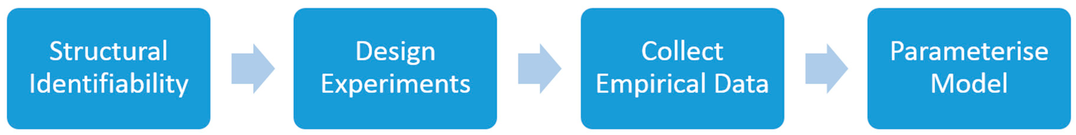
It is essential for parameters with a physical representation or meaning to be structurally identifiable, or the numerical estimates will be meaningless. Structurally identifiability analysis is an important prerequisite to modelling work, as illustrated in Figure 4.

Battery models which omit structural identifiability analyses lack rigour, greatly reducing the confidence in the accuracy of the parameter values estimated.

It is important to note that even if the models are structurally identifiable, this does not imply, or guarantee, that unique numerical estimates will be obtainable as numerical identifiability, which considers noise and sampling rate, and is a separate issue.

7. Conclusions

The structural identifiability analyses of 12 common ECMs for LIBs found in the literature reveal that:

• Seven are found to be not uniquely identifiable;
• Two are locally structurally identifiable;
• Only the three simplest models are SGI.

This greatly reduces the confidence in the accuracy of the parameter values obtained for the unidentifiable models. These models can be shown to be SGI if an additional experiment is used to estimate the OCV curve and the amount of hysteresis present. The locally structurally identifiable models can be shown to globally structurally identifiable if the local parameters are bounded without overlap. Even for the SGI models, the analysis reveals that it is advisable to perform the parameter estimation over a range of initial conditions to improve the accuracy of the parameters that rely solely on the initial conditions.

Although structural identifiability has rarely been considered in Li-ion battery modelling previously, it has implications for experiment design, system identification, and parameter estimation for all 12 models studied. The analyses performed demonstrate that it is crucial to consider the structural identifiability of LIB models before performing experiments to collect data for parameter estimation.