Data-Driven Optimization of Incentive-based Demand Response System with Uncertain Responses of Customers

1
Department of Electrical and Computer Engineering, Sungkyunkwan University, 2006 Seobu-ro, Jangan-gu, Suwon 440-746, Korea
2
Korea Electrotechnology Research Institute, 111 Hanggaul-ro, Sangnok-gu, Ansan 426-910, Korea
*
Author to whom correspondence should be addressed.
Energies 2017, 10(10), 1537; https://doi.org/10.3390/en10101537
Submission received: 5 September 2017
/
Revised: 25 September 2017
/
Accepted: 28 September 2017
/
Published: 4 October 2017
(This article belongs to the Collection Smart Grid)
Abstract
:Demand response is nowadays considered as another type of generator, beyond just a simple peak reduction mechanism. A demand response service provider (DRSP) can, through its subcontracts with many energy customers, virtually generate electricity with actual load reduction. However, in this type of virtual generator, the amount of load reduction includes inevitable uncertainty, because it consists of a very large number of independent energy customers. While they may reduce energy today, they might not tomorrow. In this circumstance, a DSRP must choose a proper set of these uncertain customers to achieve the exact preferred amount of load curtailment. In this paper, the customer selection problem for a service provider that consists of uncertain responses of customers is defined and solved. The uncertainty of energy reduction is fully considered in the formulation with data-driven probability distribution modeling and stochastic programming technique. The proposed optimization method that utilizes only the observed load data provides a realistic and applicable solution to a demand response system. The performance of the proposed optimization is verified with real demand response event data in Korea, and the results show increased and stabilized performance from the service provider’s perspective.
1. Introduction
The concept of demand response (DR), which is one of the most interesting applications in the smart grid, started from a concern with peak reduction [1,2,3]. In the time of energy crisis, customers were requested to reduce their energy consumption for the stability of the whole electricity network, at all cost. However, the focus is now moving towards energy optimization [4]. The energy market is open to demand response service providers (DRSPs). A DRSP declares its demand response capacity, and virtually generates electricity with actual load reduction through its subcontracts with many energy customers, such as factories, schools, and even households. It can actively take part in the energy market, and even bid like a generating company as if it could generate electricity, because, from the point of view of the electricity grid, energy reduction is equal to energy generation [5,6]. Basically, a DRSP gathers energy reduction capacity from customers, and provides this capacity to the energy market.
There are two possible DR models: the incentive-based model and the price-based model [6,7]. In the incentive-based model, also known as the reward-based model, if customers reduce energy consumption, they will be given financial incentives. In the price-based model, the price is controlled to induce customers to decrease demands as occasion arises. For example, demand bidding [8] and capacity market [9] are classified into incentive-based model, while time of use (TOU) [10], critical peak pricing (CPP) [11], and real time pricing (RTP) [12] are classified into price-based model [7]. In this paper, the focus is on the incentive-based model, because it is more common and widespread in the real system. For example, an incentive-based demand response system was already activated in Korea in November 2014. More than 17 DRSPs actively take part in the energy market, and the number is increasing [13].
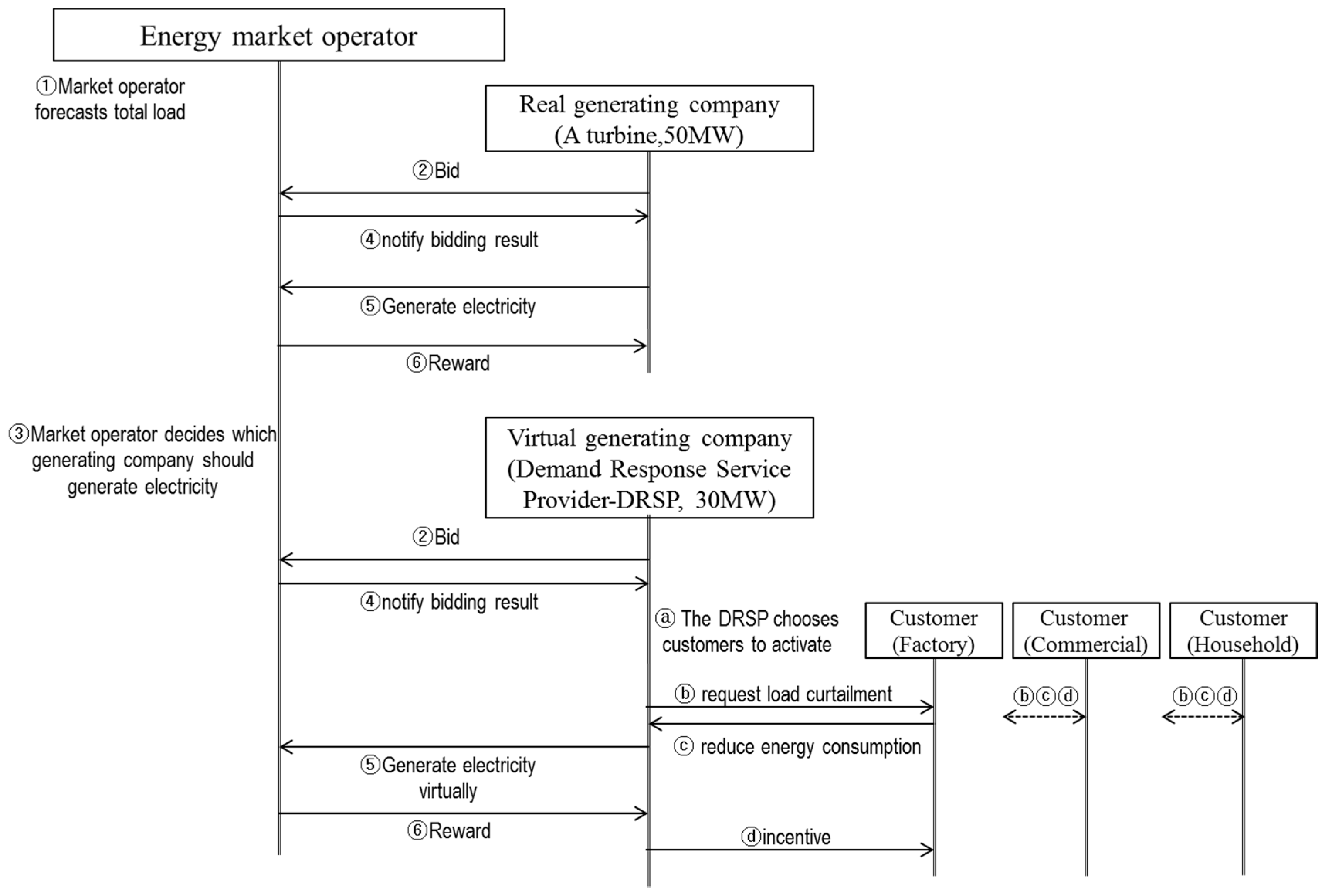
Figure 1 shows the overall structure of the demand response system that is considered in this paper [5]. As other generator companies do in the market, a DRSP can declare its generation capacity as a virtual generator. From the viewpoint of the energy system, it is assumed that 1 MW electricity generation from a turbine is perfectly equal to 1 MW load reduction from customers, as mentioned above. If a DRSP is qualified to support a certain level of load reduction, it can join the energy generation market, and do whatever a real generator company can do [14]. In a normal day, a DRSP bids in the energy market to produce virtual electricity (②), and, if it wins against other real generating companies (④), it will generate virtual electricity through load reduction and receive rewards (⑤ and ⑥). In an energy crisis, the market operator can request both real and virtual generators to produce more energy without bidding.
Figure 1 bottom right shows that there are customers who have made contracts with DRSPs. While generating virtual electricity, the DRSP requests of some of its customers that they reduce energy consumption (ⓐ and ⓑ). If customers are requested to reduce energy consumption, they curtail their consumption (ⓒ). Customers will receive incentive from their DRSP (ⓓ), which can vary, depending on the amount of load reduction and the contract between customers and their DRSP. Since DRSPs do not directly control their customers’ equipment, direct load control schemes, such as under-frequency load-shedding [15], which were usually conducted by the utility, are not included in the incentive-based demand response market.
In the energy market, a DRSP usually declares a target amount of virtual generation. It must choose some of its customers whose total reduction is close to the target amount of virtual generation (ⓐ in Figure 1), and activate them to take part in demand response (ⓑ in Figure 1). Customers also declare the amount of energy reduction that they can provide. Thus, in an ideal condition, the DRSP can easily achieve the target amount of virtual electricity by choosing the proper customers.
However, in reality, the problem is not simple, because the energy reduction of each customer is inherently uncertain. Although each customer declares its reduction capacity, it is not possible for a DRSP to force a customer to reduce its energy consumption by as much as their declared amount. Customers are usually permitted to reduce less energy than they declared, depending on their internal condition. When they do not provide the declared energy reduction, they just receive less incentive. In other words, a customer who achieved a target 1 MW energy reduction one day, might provide 0.8 MW energy reduction next day. The real environment demand response data presented in Section 5 clearly confirm that this uncertainty exists.
Due to the uncertainty of load curtailment, a DRSP cannot predict exactly how much energy reduction its customers will actually provide. Thus, it is also very difficult to choose customers whose total reduction meets the exact target amount of virtual generation. This can cause insufficient or excessive virtual electricity, which is obviously negative to DRSPs. If a DRSP can choose and activate its customers with the knowledge of uncertain responses, it can maximize its profit without the waste of resources.
In an old-fashioned demand response, which was usually conducted by a utility, the amount of reduction in each customer was usually assumed to be empirically well known by an expert demand response operator [16]. However, in practice, this only means that the average reductions of a few cooperative industrial customers are roughly known. The actual load reductions of customers can vary, day-by-day. The assumption of deterministic energy reduction may no longer be valid in the emerging demand response market system, where small commercial buildings and households that may be uncooperative are also included.
The focus of this paper is on the optimization of the customer activation list with the full consideration of the uncertainty in energy reduction of customers. The optimization problem for choosing and activating a subset of customers is formally defined and solved to maximize the DRSP’s profit. In the formulation, the amount of load curtailment from each customer is modeled using a probability distribution, instead of scalar values, such as averages. Past energy reduction data of a customer are utilized to build the probability distribution of load reduction. The uncertainty of customer response is considered using the stochastic programming technique [17] with the Monte Carlo method [18]. Finally, the problem is converted into mixed integer linear programming (MILP) to be efficiently solved. This is an innovative study that considers the uncertainty of incentive-based demand response customers for the optimization of a DRSP.
A few related studies solved similar optimization problems in the demand response application [6,16,19]. However, most of those studies assumed that the customers could provide a fixed amount of energy reduction every day, which is certainly unrealistic. In contrast, the proposed approach models and reflects the uncertainty of customers, and as a result, more reliable total energy reduction can be provided. For the prediction of each customer’s response, previous studies usually have built a detailed internal model of each customer [20,21,22,23]. For example, power storage device was modeled [20,21], air-conditioning system was modeled [22], and smart appliances were also modeled [23]. However, this is unrealistic to DRSP, because it requires a lot of information on each customer, and there are a very large number of customers. In reality, DRSPs need to optimize their strategies without detailed investigation of their customers. That is why a data-driven approach is adopted in the proposed approach. In this paper, only the observed energy consumption data are utilized, without any other details of each customer.
The performance of the proposed optimization is verified with real demand response data in Korea, unlike other studies, which were mostly based on simulated data. The result shows that the proposed optimization can achieve significant profit improvement in a real incentive-based demand response market, with very high prediction accuracy and high stability, compared to the other baselines.
The remainder of this paper is structured as follows. Section 2 summarizes the related articles. Section 3 introduces the mechanism of rewards and incentives in the incentive-based demand response market, in order to provide background knowledge of the system of concern. Section 4 provides details of the uncertainty-considered problem formulation, and the optimization of customer selection, using a data-driven approach. Section 5 verifies the performance of the proposed method with real data. Section 6 concludes the paper.
2. Related Works
Most of the literature regarding optimization of an incentive-based demand response system focuses on the modeling of the system. The concept of demand response exchange (DRX), which is similar to DRSP, has already been considered [6], and complicated parameters, such as customer operation, electric vehicle load, and distributed generation, as well as parameters related to the core of demand response, were included in the modeling [19]. A retail electricity provider that includes demand response concept is also modeled in detail [16]. However, these papers did not consider the uncertainty of customer responses, which is the main focus of this research. Regarding the price-based demand response system, price-responsiveness has been extensively studied for setting optimal price strategy. In the literature, customers’ preferences on price are generally modeled [24], household’s utility function is modeled [25], and time-utility model is introduced to simulate price elastic behaviors of aggregated load [26]. Optimization of price settlement based on iterative information exchange is also proposed [27] and a special effect called rebound-peak is also considered [28]. The modeling is usually more complex in this type of system, because it simultaneously contains price and its response. Although price-responsiveness is a very important topic in the demand response domain, it is not directly related to our research, because the focus of this work is on an incentive-based system.
Uncertainty in energy systems has been considered in the literature in many applications [29], and it has been well reviewed [30]. Although many research efforts exist on the uncertainty concept of an energy system, the uncertainty considered is related to the operation of each application system, such as renewables or electric vehicles. The literature does not cover the uncertainty of incentive-based demand response well.
Apart from the optimization of a DRSP, scheduling of energy consumption in a single customer with its modeling has been extensively studied. Usually, the optimization target was the minimization of the energy bills of customers [31,32,33]. Power storage devices were considered in extension of the ordinary demand response [20,21], and user inconvenience was also considered [32]. In the modeling of smart appliances, uncertainty was also included [23]. However, these studies focused on the efficiency of a single customer, and did not consider a DRSP as an optimization target. Hussain’s recent work reviewed many other related research efforts in this area of optimizing schedules for a specific customer [34].
A game theoretic approach that considers interaction between customers was also proposed. It calculates the optimized response schedule for each customer with Nash equilibrium [35]. However, this type of research is different from our DRSP system, because their goal is to optimize the system on both sides, i.e., the DRSP’s side and the customers’ side; and it also assumes customers’ modeling with more information. In contrast, in this paper, the focus is on the optimization inside a DRSP, and a data-driven approach that uses only energy reduction data from customers is applied.
Because we start from energy data in the real environment, data-driven machine learning approaches to related energy applications are also mentioned here, even though they are not directly related to demand response application. The most traditional and related research to demand response is short term load forecasting. Various mechanisms and machine learning techniques have been applied and summarized in the literature [36]. Although the prediction of load is surely one of the key technologies, it is not closely related to our scope, because the focus is not on the consumption of energy for a normal day, but on the reduction of energy for a DR event day. The clustering of electricity customers is also considered a serious issue in many studies that consider energy consumption and demand response. Although the clustering can be a pre-stage for demand response applications [37,38], it is also not closely related to our research, because at this time, no clustering mechanism is considered.
Calculation of the customer baseline load (CBL) is another important issue, because energy reduction is measured based on the CBL. The amount of energy reduction by a customer is defined as the difference between the customer baseline load, and the real energy consumption on the event day. The customer baseline load is usually determined by averaging the energy consumption of the past five or ten days [5]. Therefore, some research efforts focus on the precise estimation method of CBL [39,40]. In our research, the most recent energy consumption data on normal days is chosen as a CBL, because our work is not related to precise CBL estimation, but is related to the amount of energy reduction.
3. Structure of the Incentive-Based Demand Response Market
This section describes the overall structure of the incentive-based demand response market, in order to help readers understand the incentive-based demand response system.
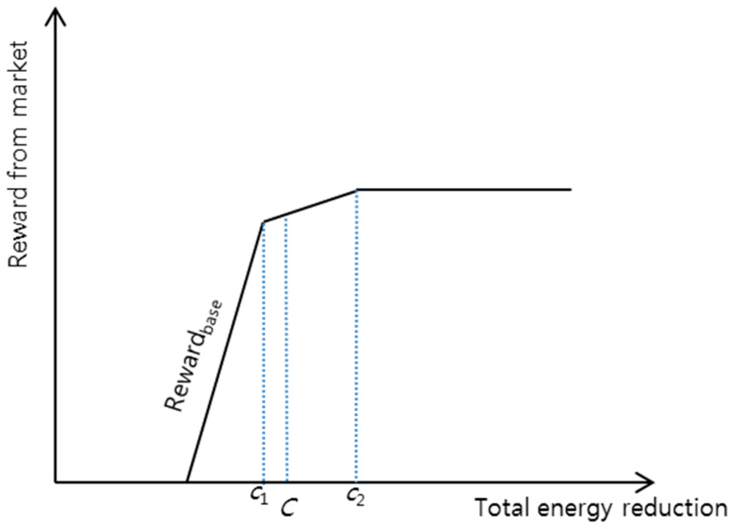
Similar to other generating companies, a DRSP receives reward from the market when it generates virtual electricity. However, the reward is somewhat different from that of ordinary generating companies. Figure 2 shows an example of a reward function. A DRSP promises to reduce the energy by as much as C, the reduction capacity. The DRSP will receive a unit price for every kWh that it generates, but should pay serious penalties if it provides less energy reduction than the predetermined amount (), which is a little bit smaller than C. In Korea, the penalty is at least twice as much as the unit price given to a DRSP, because insufficient virtual generation is considered to be a very serious protocol violation in the electricity system. Assume that the price of 1 kWh virtual generation is $0.1 and the threshold () is 97% of declared capacity. If a DRSP declares 100 kWh of energy reduction and it provides 100 kWh reduction, it will receive $10 for the virtual generation. However, if it reduces 80 kWh, only $4.6 will be given to the DRSP, because the energy reduction is less than the threshold (97 kWh) and 17 kWh of insufficient energy reduction will cause at least $3.4 of penalty to the DRSP. This penalty will be subtracted from $8 and the final reward will be $4.6. If the amount of reduction is less than 64.66 kWh, the calculated reward will be $0 because of serious penalty. On the other hand, a DRSP does not receive any additional reward, even if it reduces more than another predetermined level of energy reduction () that is larger than C. This is because the energy market and the energy network cannot accept unlimited virtual electricity generation. Therefore, the slope of the overall reward function changes at these two threshold points, as shown in Figure 2. This reward function is reasonable, because it is hard to exactly reduce consumption by as much as the declared capacity, due to the non-determinability of virtual generation. Although Figure 2 may not thoroughly present every small complicated detail of the real reward function, the shape of the reward function is practical, and exactly reflects the real reward function in Korea.
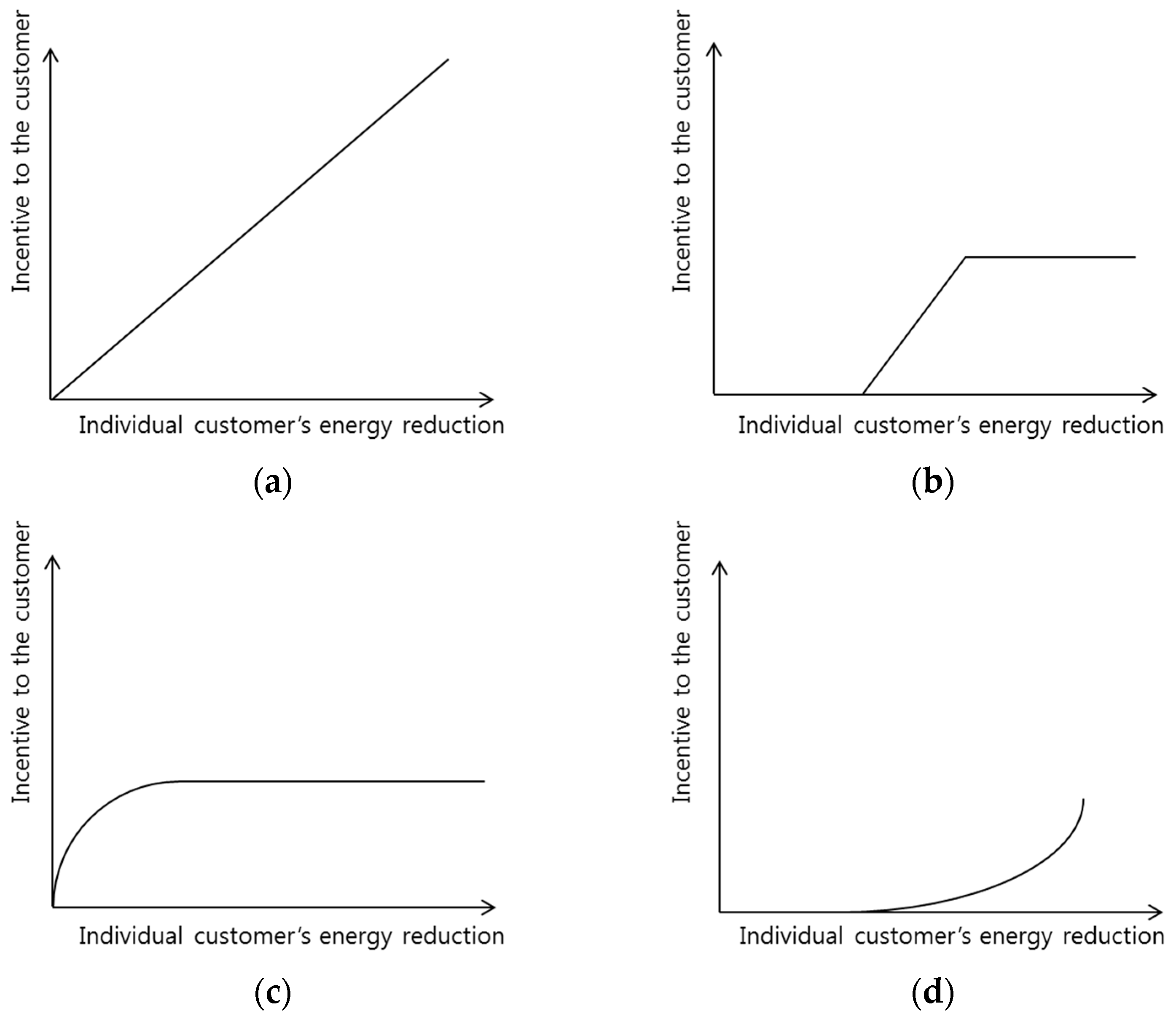
Unlike real generating companies, a DRSP must pay incentives to their customers to promote their participation in demand response events. The amount of incentives to each customer is up to the contract between the DRSP and its customer. The incentive contract is fixed when a customer agrees to join a DRSP. Figure 3 shows some possible examples of incentive contracts. In a DRSP, different incentive contracts can be applied to different customers. Figure 3a shows the most widely acceptable contract, which provides a linear incentive to energy reduction [16]. Figure 3a is simple, and very advantageous to customers. Figure 3b is another popular incentive contract under which a customer receives incentives only when it provides a predefined energy reduction [41]. Furthermore, an upper bound of the incentive also exists in this contract. It is relatively beneficial to a DRSP, because it tends to force the customer to provide its declared capacity. Other imaginary types of incentive contracts, as shown in Figure 3c,d, are also possible. These figures are presented to show that there is no limitation on the incentive contract between a customer and a DRSP. Although the exact types of incentive contracts are internal and confidential information of a DRSP, Types (a) and (b) are the most widely accepted incentive contract functions in Korea. To gather many customers, the incentive contract should be beneficial to customers and Type (a) will be more popular in the future.
In Figure 2 and Figure 3, it is obvious that somehow a DRSP must optimize energy reduction. If a DRSP fails to provide sufficient reduction on the request, the penalty will be catastrophic. If it provides too much reduction, the incentives given to its customers will increase, and its profit will decrease. Therefore, the problem of a DRSP in these circumstances is to precisely predict the energy reduction of each customer on an event day, and to determine the optimized participation list of its customers, so that the total energy reduction maximizes the profit. The essential part of this process is how to solve the customer selection problem, considering the uncertainty in energy reduction of each customer, as mentioned in Section 1.
4. Optimization of Customer Selection with the Uncertain Responses of Customers
4.1. Problem Definition
The goal of a DRSP is to find the optimal selection of customers that maximizes the profit of the DRSP. The profit is simply calculated by subtracting the incentives from the reward. Therefore, the problem is defined as in Equation (1):
where is the amount of energy reduction that customer i will provide; is the 1 or 0 binary decision variable that denotes inclusion or exclusion of customer i in the participation list; N is the number of customers; is the function shown in Figure 2; is one of the incentive functions shown in Figure 3; and Ccritical is a constant.
The goal is similar to Parvania’s work [19], except that, in our work, customer responses are uncertain variables. Furthermore, the reward and incentive function is not necessarily linear in our work. The constraint in Equation (1) is related to the license revoking condition, because the license to join the energy market may be revoked if the service provider does not provide a pre-defined threshold capacity, which is 70% of the declared one in Korea. Although the equation seems relatively simple, it contains the core of demand response, and perfectly fits the currently running electricity generation market presented in Section 3, in which a DSRP is considered to be a virtual generating company. If a DRSP physically owns distributed generations (DG) and energy storage systems (ESS), the formulation of the problem will be more complicated with related parameters. If a DRSP serves as both virtual generating company and retail electricity provider, the modeling of the problem is also more complicated because it has to simultaneously generate and consume electricity. However, in this paper, the focus is not on the modeling of various additional considerable parameters, but on the inclusion of uncertainty in the energy reduction of the customer. In the explained incentive-based demand response market, a DRSP only serves as a virtual generating company with its customers. If necessary, other parameters, such as DG, ESS, and time, can be integrated into the proposed formulation without much effort, because they are already well designed in the previous works [6,16,19].
4.2. Problem Solving with Stochastic Programming
Because the amount of energy reduction is variable in Equation (1), stochastic programming must be considered to find an optimal solution. The solution is converted to fixed deterministic form using the Monte Carlo method [18]. In other words, K scenarios are generated and the average profit of those scenarios is calculated. In each scenario, instantiation of variables is necessary. In our work, this is conducted according to the data-driven prediction method, which is based on probability distribution. The prediction method is described in detail in the following subsection. In the current subsection, it is just assumed that a data-driven method can generate a sample every time. The converted equation is presented in Equation (2). The amount of energy reduction, , is now converted to a constant, , where j represents each scenario, and K is the number of total scenarios. At this stage, the latter part of Equation (2) (the sum of all incentives) is considered to be linear, regardless of the real shape of the incentive functions, because the only remaining variable, , is a 1 or 0 binary variable, which can be placed outside of the incentive function:
However, the first part () of Equation (2) still includes a nonlinear part, which makes optimization difficult. At this step, it is assumed that the reward function is linear in every interval, as shown in Figure 2. This assumption is reasonable, because an equal unit price is usually applied to electricity. Even if it is not linear, it can still be solved with more complex programming technique. This is further mentioned at the end of this section. With this simple assumption, Equation (2) can be rewritten as Equation (3) by adding the continuous non-negative variables y and z. In the literature, the knapsack problem [42] with unlimited boundary was solved by adding a single continuous variable [43], and this concept is applied to our problem, in order to make the equation linear. In our problem, 2K continuous variables are added, instead of one variable, because K scenarios are included in the calculation.
represents a linear function in the first interval in Figure 2, and and are breaking points that are also presented in Figure 2. and are non-negative constant values that are calculated as the difference between slopes in Figure 2. When is smaller than , and are both going to be 0. When exceeds , will have a certain value according to the second and third constraints, and plays a role in the optimization. If exceeds , will also play the role of maximizing the object function according to the second and the last constraints.
As a result, it is perfectly in the form of mixed integer linear programming with N binary variables, s, 2K continuous variables, s and s, and 5K constraints (the conditions of Equation (3)). Any commercial or academic mixed integer linear programming algorithm can be utilized to find the solution.
By applying the proposed optimization method, highly unpredictable or unreliable customers will be excluded from the participation list. For example, a customer who provides zero energy reduction one day and 100% energy reduction the next day will be excluded, because the inclusion of such customers easily causes insufficient or excessive reduction, both of which reduce the total profit.
In the proposed optimization, the optimal solution cannot be guaranteed, because integer programming is a nondeterministic polynomial (NP) time hard problem. However, MILP has many fast and efficient algorithms in the literature that find the near optimal point. Without any limitation on the form of the reward function, the problem in most cases can be reduced to mixed integer quadratic programming (MIQP), or at least can be reduced to mixed integer nonlinear programming (MINLP). The problem can still be solved with related approximation algorithms, even though it may take much longer, and provide more inaccurate performance than MILP. Usually the equation will be linear, because a DRSP is rewarded with equal unit price.
As with any problem that employs a data-driven approach, an over-fitting problem can also arise in our proposed optimization. In data-driven approaches, the system is optimized based on the training data (past data), but the result is evaluated based on the test data (future data). The difference between the training data and the test data will give rise to an over-fitting problem: that if our system is over-optimized with respect to the training data, the performance of the optimization may degrade. In our work, this over-fitting problem is alleviated with the early stopping in the optimization process. Section 5 discusses the effect of over-fitting, with experimental results.
4.3. Prediction of Energy Reduction for Each Customer
This subsection describes the prediction method of each customer’s response. Customers’ energy reduction data from past experience are used, because a DRSP can obviously acquire them, although the number of event days may not be large enough. Only these data are directly utilized in the prediction.
To predict the amount of energy reduction of each customer, it is proposed to estimate the probability distribution of each customer’s energy reduction. The reason why we choose to predict energy reduction in the form of a probability distribution is that the probability distribution inherently provides information of uncertainty. Furthermore, it is certain that a set of the reduction history of each customer can build a probability distribution, even though the shape is not known. With this assumption, each customer is considered to reduce its energy consumption according to the distribution, such as Gaussian, Gaussian mixture model [44], categorical distribution [45], or any other distribution. The distribution parameters can be estimated using only observed samples. Of course, in our case, the amounts of energy reductions in past event days are observed samples. No internal information of customers is required at all, and any type of customer, such as a small building or household, can be modeled. Furthermore, the modeling of probability distribution is perfectly applicable to the problem defined in the previous subsection, because in probability distribution, sampling with uncertainty is natural. It may seem that the prediction of future from past data is relatively simpler than modeling the internal behavior or each customer. However, it needs no information, and no complicated assumptions.
Three distributions are considered in the prediction of customers’ responses, which are the Gaussian, Gaussian mixture, and categorical distributions. First, the Gaussian distribution is one of the simplest and most well-known probability distributions. Although it is a very effective and attractive way of modeling data, it may not be appropriate in our case. According to our analysis of customers’ response, only some of the energy reduction histories of the customers are similar to the Gaussian distribution. In our real data from Korea, only 37.8% of customers passed the Shapiro–Wilk normality test [46] with the data of 13 event days. This means that most customers do not follow Gaussian distribution. The reason is that energy reduction is highly dependent on each customer’s circumstance. The manager of a factory may decide to turn off most of its load on one day, but can decide not to turn off any of its load on the next day, because of its production schedule, etc. In fact, this case is similar to a multimodal distribution. The Gaussian mixture model (GMM) is considered for this kind of multimodal distribution, because it provides the ability to model multiple peaks in its distribution. If a factory manager has three strategies (all, some, and none), a mixture of three Gaussian distributions can model the result well. In the experimental section, GMM is configured to a mixture of three Gaussian distributions. Third, categorical distribution is also considered in our work. With categorical distribution, each past reduction datum from a customer has equal probability of being selected in the future; and, if it is selected, it provides the exact same energy reduction of that selected day. This categorical distribution is acceptable, especially if the past reduction data are not enough to estimate the parameters of a certain distribution model.
5. Experiment
5.1. Data Set and Experimental Setup
The data used in this paper are real demand response results in 2011, in Korea. There are 13 event days. Although the number of data may be considered insufficient compared to the usual data size for a data-driven method, this is inevitable, because demand response itself is an unusual situation. The customers were required to reduce energy consumption from 10:00 to 11:30 in the morning. In 2011, there was no demand response market available, and the only goal was to reduce nation-wide energy consumption. Even though the data are not based on the assumption of DRSPs, they reflect the responses of actual customers, and can show the optimization possibility. Unlike other studies that focus on a specific type of customers, the customers in this research consist of 307 various sites, such as schools, shopping centers, and factories. This is because demand response can be applied to any kind of customer. At least in Korea, the type of customer is no longer a concern if a DRSP can provide minimum reduction capacity. For simplicity, the incentive functions are assumed to be linear and identical for all customers. The declared DR capacity (C in Figure 2) is set to 83% of the average reduction in our experiment. This means that the total average reduction is set to the saturation point in the reward function. This is a reasonable scenario from the fact that a DRSP always declares a smaller capacity than the average achievable capacity, because the amount of energy reduction is not at all guaranteed. The price of electricity is set to the default value of the Korea energy market.
Regarding the optimizer, Gurobi optimizer [47] with its default branch-and-bound method, which can solve MILP effectively, is utilized. The branch-and-bound method builds the tree of candidate solutions and estimates the upper and the lower bounds on the solution. While traversing the tree of candidate solutions, it prunes some of the branches based on the estimated upper and lower bounds [48]. An MILP problem, with 307 binary variables, 1000 continuous variables, and 2500 constraints (K = 500), was solved in a few seconds with this method. The presented result is the average of 10 independent trials, because the optimization itself is not deterministic. At each trial, the participation list is optimized with some training event days, and the real profit is calculated using the remaining test event days, according to the participation list generated by the optimization. Unless the number of training days is mentioned in the experiment, the first eight days of data are used as training data, and the remaining five days of data are used as test data.
5.2. Experimental Results
Firstly, the characteristics of customers are discussed. A customer is presented as a circle in Figure 4. The X-axis represents the training-day energy reduction ratio, which is defined as the consumption reduction divided by the maximum possible reduction. For example, if a customer usually consumes 10 kWh, and on the event day it consumed 8 kWh, the reduction ratio is 0.2. The Y-axis represents the test-day energy reduction ratio. The sizes of circles are absolute values of average consumption. In Figure 4, it is certain that past experience provides reasonable prediction of the future, because most of the circles are located on the diagonal line. Of course, there are customers who show different patterns between the training data and test data.
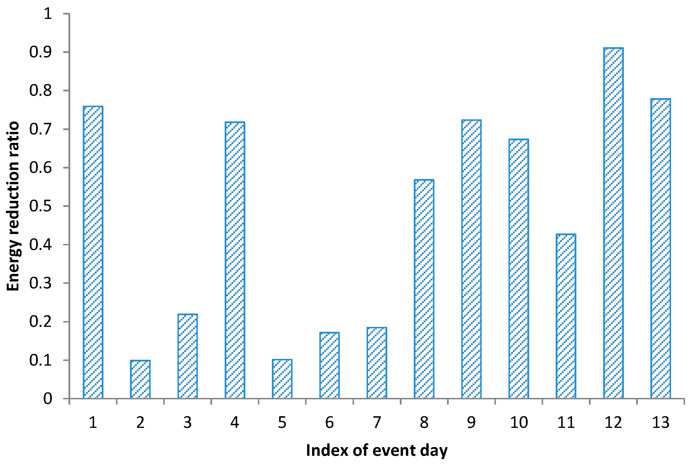
Figure 5 shows the daily energy reduction ratio of a customer to provide insight into the detail of its individual response. The customer’s reduction pattern dramatically varies day-by-day as mentioned in Section 1. This customer reduced only 10% of its load on Day 2, and reduced 90% of its load on Day 12. From the result, there is no doubt that the distribution of each individual’s energy reduction may not be simple, and, in reality, some customers provide very uncertain energy reductions.
Before the performance of our proposed method is compared to those of other baselines, two preliminary tests are conducted to determine the two parameters that were mentioned earlier: the optimization stop condition for the prevention of over-fitting, and the number of scenarios in stochastic programming. These preliminary tests of the proposed optimization are conducted with the assumption of the categorical distribution of customers’ responses.
First, Figure 6 shows the necessity of setting a stop condition in the proposed MILP optimization due to over-fitting. Unlike normal optimization, an over-fitting problem may arise in the proposed solution, because optimization will find the best solution for training data that do not show equal distribution to the test data. With setting some gap in the stop condition, MILP will stop when the difference ratio between the expected optimal value and the current objective value is smaller than a designated gap. This simple step will provide generalization ability in the data-driven approach, and prevent the model from over-fitting to training data. Figure 6 shows that the average profit of the proposed method without a stop condition is degraded against that with a stop condition, even though the predicted profit, which is equal to the objective of optimization, is maximized without a stop condition. It is certain that a 2% solution gap in the stop condition of the optimizer is sufficient to provide generalization ability in our data. The error bars in Figure 6 show the maximum profit and minimum profit on five test data, and they also show reasonable results with 2% or more gaps.
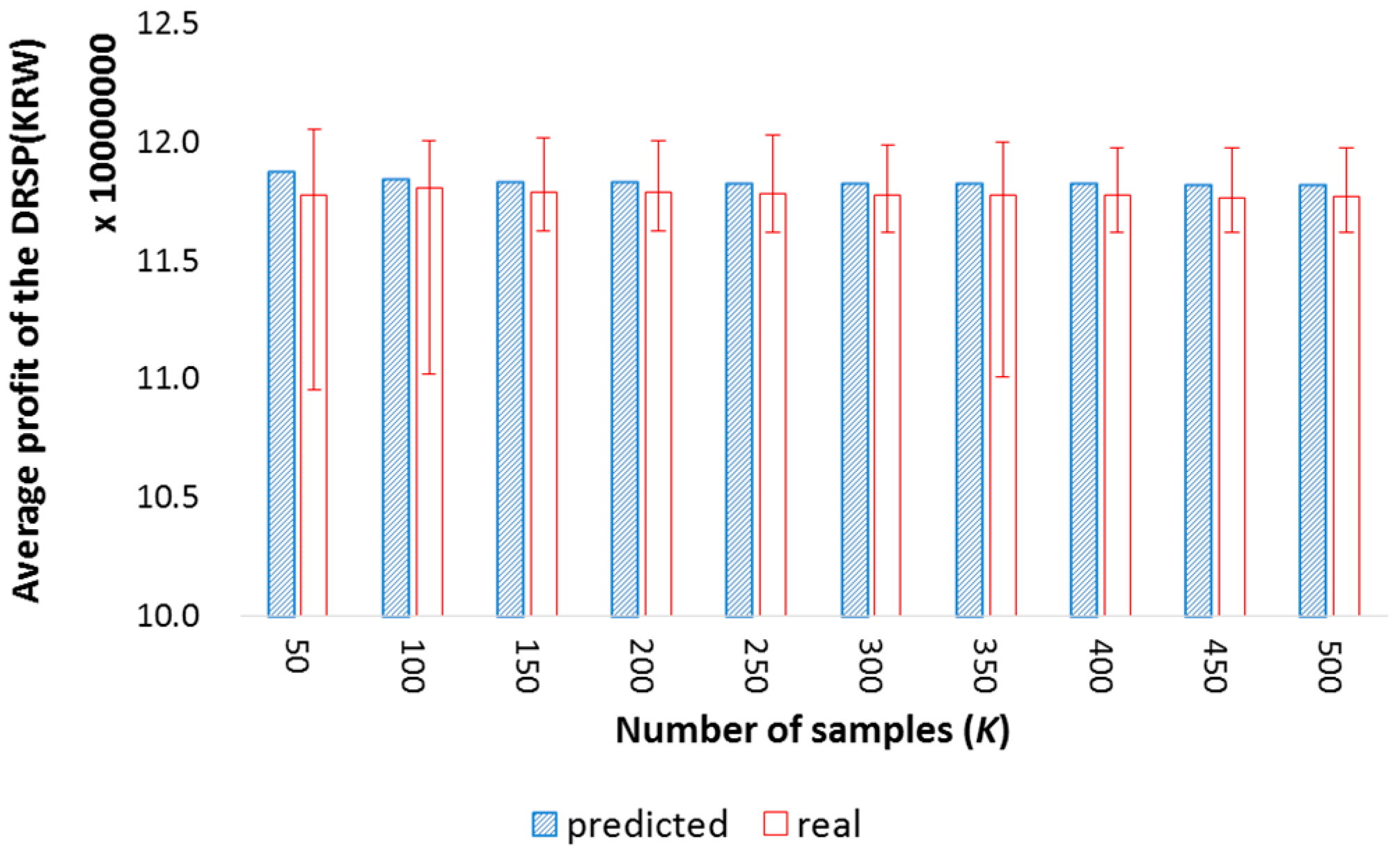
Second, Figure 7 shows the effect of the number of scenarios (K). To cover all the possibilities with eight training days and 307 customers, 8307 scenarios are necessary, which is not feasible. If the number of scenarios is too small, the optimization will provide an inaccurate result; and if it is too large, it will cause too many variables and constraints in the modeling, because the proposed equation needs 2K continuous variables and 5K constraints. With our data, 50 or 100 scenarios are not enough to provide a stable result, because the difference between the predicted profit and the real test profit is large, and the max-min fluctuation of the real profit presented by the error bar is also large. The cases with more than 150 scenarios provide more stable and improved results in most cases. Although there are mechanisms to make efficient scenarios in stochastic programming [29,49,50], such programming is not considered here, because the random samples are enough to provide effective results with our data.
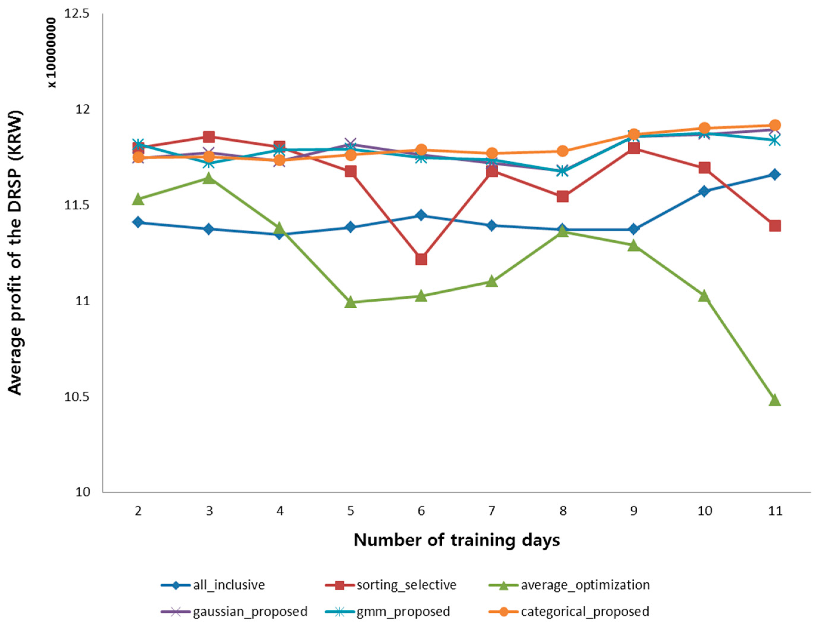
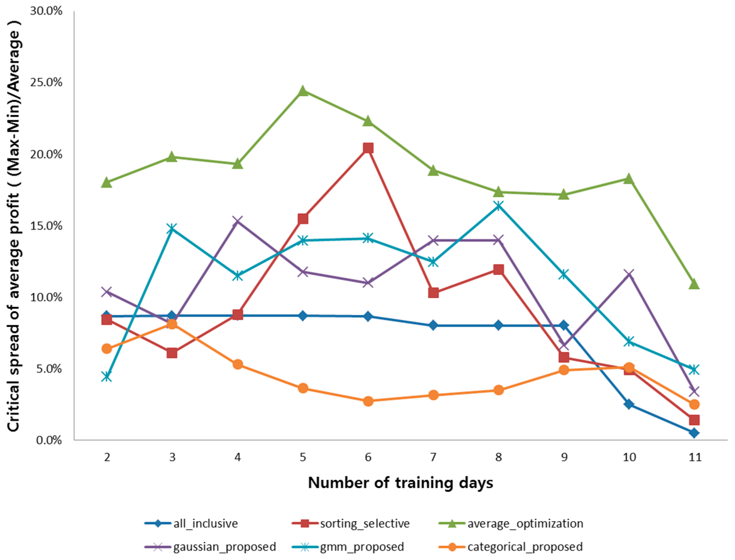
Finally, Figure 8, Figure 9 and Figure 10 compare the performance of the proposed optimization to other baselines. The first baseline method is “all-inclusive”, where event signals are sent to all the customers. Another baseline is “sorting-selective”, in which event signals are sent to some customers based on their total energy consumption. The customers are sorted by their average energy reduction in descending order, and they are chosen one-by-one, until the expected profit of DRSP is maximized with a greedy approach. The third baseline is “average-optimization”. In this method, the average reduction in the training data of each customer is treated as the prediction of future reduction, and the profit is optimized with integer programming. In other words, in this baseline, the uncertainty of customers is not included, to show the necessity of uncertainty information, in comparison to the proposed optimization method. The results of the proposed method are presented each with its assumed probability distribution (Gaussian, GMM, and categorical). The X-axis represents the number of consecutive training days used in the experiment. The proposed optimization in Figure 8, Figure 9 and Figure 10 employed K = 250 and gap = 2%.
The average profits of the proposed optimization clearly show improved results on the test data compared with all of the other baselines in Figure 8. The exception happens only when the number of training data is smaller than four days; the sorting-selective scenario provides a slightly higher result in these cases. This is because the trained model may not be correct, due to a lack of training data. If the number of training data is larger than four days, there is no doubt that the proposed methods improve the results.
Selecting the probability distribution of energy reduction is also an important step in the proposed optimization. Among Gaussian, GMM, and categorical distribution, categorical distribution shows the best performance. The reasonable explanation is that the Gaussian and GMM may not be applicable to all of the customers. Some of them may even follow a uniform distribution, or any other unknown distribution. As mentioned above, only 37.8% of our customers passed the Shapiro–Wilk normality test [46]. However, categorical distribution can model the unknown probability distribution well, because it uses only observed value, without any assumption of the shape of distribution. Another reason can be the lack of training data. Although estimating probability distribution needs many data samples, demand response itself is an event that rarely happens, which cannot provide many training data. Categorical distribution can be better, because it does not estimate distribution, but directly uses historical energy reduction data.
The overall average profit improvement of “categorical-proposed” is 3.2% compared to “all-inclusive”, 1.4% compared to “sorting-selective”, and 5.6% compared to “average-optimization”, respectively. With five or more training days that imply acceptable training data size, profit improvement is more amplified. This profit improvement is significant, and it will also be amplified if the declared capacity is not carefully selected by the expert. Furthermore, the improvement will be even more amplified in the future, because many unreliable small customers, such as small offices or commercial buildings, tend to be included in the demand response customers.
Figure 9 shows the prediction error of various methods. The prediction error is the difference between the predicted profit and the real profit. We present the mean absolute percentage error (MAPE) of profit predictions in Figure 9. The predicted profit calculated in the optimization process is inherently different from the real profit and the difference between these two should be minimized in order to help a DRSP decide its strategy. The proposed optimization clearly provides smaller error than all the other baseline cases. In particular, the proposed method with categorical distribution shows the smallest average error among all the other methods. The overall average of MAPE in the proposed optimization is minimized to 1.2% with categorical distribution. The three other baseline methods’ prediction errors are 2.3%, 4.0%, and 7.3%, respectively. It is certain that a small prediction error is also essential in the decision process of a DRSP. With the result of 5–8 training days, which means reasonable splits of training and test data, the prediction error in the proposed optimization with categorical distribution will be decreased to 0.8%.
Figure 10 shows the critical spread, which is defined as the difference of maximum profit and minimum profit divided by the average profit in the test result. This is presented, because it can reveal the worst case error of the experiment. Similar to Figure 8 and Figure 9, the proposed optimization with categorical distribution shows very low value. This means that the proposed method with categorical optimization provides extremely stable results. The overall average of critical spread in the proposed optimization with categorical distribution is 4.5%. The three other baseline methods’ critical spreads are 7.0%, 9.3%, and 18.6%, respectively. With the result of 5–8 training days, the critical spread in the proposed optimization will be decreased to 3.2%.
The results clearly show that the proposed data-driven optimization provides improved performance in all aspects such as acquired profit, prediction accuracy, and stability that are essential to DRSPs in the real incentive-based demand response systems.
6. Conclusions
The concept of peak reduction in demand response has been extended to virtual generators that are identical to real generators. In this circumstance, optimization of the demand response is essential for effective energy reduction. The energy reduction of customers must be predicted and optimized for maximum efficiency.
We formally defined and solved the customer selection problem of a DRSP that includes the unreliability of energy reduction. The uncertainty is considered with the modeling of probability distribution, and the problem was converted to MILP, with an assumption that was relatively easy to solve. The experimental results showed that the proposed optimization with the assumption of categorical distribution provided improved performance, in terms of profit, predictability, and stability.
Although the proposed optimization focused on the customer selection problem, many other decision parameters, such as the shape of incentive functions and the amount of declared capacity, can also be easily included in the optimization framework. In conclusion, it is certain that the proposed optimization framework can be treated as a turning point for DRSPs: from a speculative decision of strategy, to a mathematically informed one.
Acknowledgments
This work was supported by the KERI Primary research program of MSIP/NST (No. 17-12-N0101-07). This work was also supported by the National Research Foundation of Korea (NRF) grant funded by the Korea government (MSIP) (No. NRF-2016R1A2B4015820).
Author Contributions
Jimyung Kang mainly conducted this research, while Jee-Hyong Lee advised on this research as an advising professor.
Conflicts of Interest
The authors declare that they have no conflict of interest.
References
- Benefits of Demand Response in Electricity Markets and Recommendations for Achieving Them. Available online: https://eetd.lbl.gov/sites/all/files/publications/report-lbnl-1252d.pdf (accessed on 29 September 2017).
- Agency, I.E. The Power to Choose: Demand Response in Liberalised Electricity Markets; OECD: Paris, France, 2003. [Google Scholar]
- Albadi, M.H.; El-Saadany, E.F. A summary of demand response in electricity markets. Electr. Power Syst. Res. 2008, 78, 1989–1996. [Google Scholar] [CrossRef]
- Simmhan, Y.; Aman, S.; Cao, B.; Giakkoupis, M.; Kumbhare, A.; Zhou, Q.; Paul, D.; Fern, C.; Sharma, A.; Prasanna, V.K. An Informatics Approach to Demand Response Optimization in Smart Grids; Technical Report; University of Southern California: Los Angeles, CA, USA, 3 March 2011. [Google Scholar]
- Korea Energy Market Operation Protocol (In Korean). Available online: http://www.kpx.or.kr (accessed on 18 September 2017).
- Nguyen, D.T.; Negnevitsky, M.; Groot, M. Pool-based demand response exchange—Concept and modeling. IEEE Trans. Power Syst. 2011, 26, 1677–1685. [Google Scholar] [CrossRef]
- Albadi, M.H.; El-Saadany, E.F. Demand Response in Electricity Markets: An Overview. In Proceedings of the 2007 IEEE Power Engineering Society General Meeting, Tampa, FL, USA, 24–28 June 2007. [Google Scholar]
- Liu, Y.; Guan, X. Purchase allocation and demand bidding in electric power markets. IEEE Trans. Power Syst. 2003, 18, 106–112. [Google Scholar]
- Aalami, H.A.; Moghaddam, M.P.; Yousefi, G.R. Demand response modeling considering interruptible/curtailable loads and capacity market programs. Appl. Energy 2010, 87, 243–250. [Google Scholar] [CrossRef]
- Atkinson, S.E. Responsiveness to time-of-day electricity pricing: First empirical results. J. Econom. 1979, 9, 79–95. [Google Scholar] [CrossRef]
- Herter, K. Residential implementation of critical-peak pricing of electricity. Energy Policy 2007, 35, 2121–2130. [Google Scholar] [CrossRef]
- Taylor, T.N.; Schwarz, P.M.; Cochell, J.E. 24/7 hourly response to electricity real-time pricing with up to eight summers of experience. J. Regul. Econ. 2005, 27, 235–262. [Google Scholar] [CrossRef]
- Demand Response Service System (In Korean). Available online: http://dr.kmos.kr/web/list.do (accessed on 30 September 2017).
- Rahimi, F.; Ipakchi, A. Demand Response as a Market Resource under the Smart Grid Paradigm. IEEE Trans. Smart Grid 2010, 1, 82–88. [Google Scholar] [CrossRef]
- Delfino, B.; Massucco, S.; Morini, A.; Scalera, P.; Silvestro, F. Implementation and comparison of different under frequency load-shedding schemes. In Proceedings of the Power Engineering Society Summer Meeting, Vancouver, BC, Canada, 15–19 July 2001. [Google Scholar]
- Ghazvini, M.A.F.; Faria, P.; Ramos, S.; Morais, H.; Vale, Z. Incentive-based demand response programs designed by asset-light retail electricity providers for the day-ahead market. Energy 2015, 82, 786–799. [Google Scholar] [CrossRef]
- Birge, J.R.; Louveaux, F. Introduction to Stochastic Programming; Springer Science & Business Media: Berlin, Germany, 2011. [Google Scholar]
- Kalos, M.H.; Whitlock, P.A. Monte Carlo Methods; John Wiley & Sons: San Francisco, CA, USA, 2008. [Google Scholar]
- Parvania, M.; Fotuhi-Firuzabad, M.; Shahidehpour, M. Optimal demand response aggregation in wholesale electricity markets. IEEE Trans. Smart Grid 2013, 4, 1957–1965. [Google Scholar] [CrossRef]
- Adika, C.O.; Wang, L. Smart charging and appliance scheduling approaches to demand side management. Int. J. Electr. Power Energy Syst. 2014, 57, 232–240. [Google Scholar] [CrossRef]
- Mishra, A.; Irwin, D.; Shenoy, P.; Kurose, J.; Zhu, T. Greencharge: Managing renewable energy in smart buildings. IEEE J. Sel. Areas Commun. 2013, 31, 1281–1293. [Google Scholar] [CrossRef]
- Gao, D.; Sun, Y.; Lu, Y. A robust demand response control of commercial buildings for smart grid under load prediction uncertainty. Energy 2015, 93, 275–283. [Google Scholar] [CrossRef]
- Chen, X.; Wei, T.; Hu, S. Uncertainty-aware household appliance scheduling considering dynamic electricity pricing in smart home. IEEE Trans. Smart Grid 2013, 4, 932–941. [Google Scholar] [CrossRef]
- Samadi, P.; Mohsenian-Rad, A.-H.; Schober, R.; Wong, V.W.; Jatskevich, J. Optimal real-time pricing algorithm based on utility maximization for smart grid. In Proceedings of the 2010 First IEEE International Conference on Smart Grid Communications (SmartGridComm), Gaithersburg, MD, USA, 4–6 October 2010. [Google Scholar]
- Li, N.; Chen, L.; Low, S.H. Optimal demand response based on utility maximization in power networks. In Proceedings of the Power and Energy Society General Meeting, Detroit, MI, USA, 24–29 July 2011. [Google Scholar]
- Yu, R.; Yang, W.; Rahardja, S. A statistical demand-price model with its application in optimal real-time price. IEEE Trans. Smart Grid 2012, 3, 1734–1742. [Google Scholar] [CrossRef]
- Qian, L.P.; Zhang, Y.J.A.; Huang, J.; Wu, Y. Demand response management via real-time electricity price control in smart grids. IEEE J. Sel. Areas Commun. 2013, 31, 1268–1280. [Google Scholar] [CrossRef]
- Li, Y.; Ng, B.L.; Trayer, M.; Liu, L. Automated residential demand response: Algorithmic implications of pricing models. IEEE Trans. Smart Grid 2012, 3, 1712–1721. [Google Scholar] [CrossRef]
- Conejo, A.J.; Carrión, M.; Morales, J.M. Decision Making under Uncertainty in Electricity Markets; Springer: Berlin, Germany, 2010. [Google Scholar]
- Soroudi, A.; Amraee, T. Decision making under uncertainty in energy systems: State of the art. Renew. Sustain. Energy Rev. 2013, 28, 376–384. [Google Scholar] [CrossRef]
- Erol-Kantarci, M.; Mouftah, H.T. Wireless sensor networks for cost-efficient residential energy management in the smart grid. IEEE Trans. Smart Grid 2011, 2, 314–325. [Google Scholar] [CrossRef]
- Setlhaolo, D.; Xia, X.; Zhang, J. Optimal scheduling of household appliances for demand response. Electr. Power Syst. Res. 2014, 116, 24–28. [Google Scholar] [CrossRef]
- Fakhrazari, A.; Vakilzadian, H.; Choobineh, F.F. Optimal energy scheduling for a smart entity. IEEE Trans. Smart Grid 2014, 5, 2919–2928. [Google Scholar] [CrossRef]
- Hussain, I.; Mohsin, S.; Basit, A.; Khan, Z.A.; Qasim, U.; Javaid, N. A Review on Demand Response: Pricing, Optimization, and Appliance Scheduling. Procedia Comput. Sci. 2015, 52, 843–850. [Google Scholar] [CrossRef]
- Mohsenian-Rad, A.-H.; Wong, V.W.; Jatskevich, J.; Schober, R.; Leon-Garcia, A. Autonomous demand-side management based on game-theoretic energy consumption scheduling for the future smart grid. IEEE Trans. Smart Grid 2010, 1, 320–331. [Google Scholar] [CrossRef]
- Chow, J.H.; Wu, F.F.; Momoh, J.A. Applied Mathematics for Restructured Electric Power Systems; Springer: Berlin, Germany, 2005. [Google Scholar]
- Kang, J.; Lee, J.-H. Electricity customer clustering following experts’ principle for demand response applications. Energies 2015, 8, 12242–12265. [Google Scholar] [CrossRef]
- Jin, C.H.; Pok, G.; Lee, Y.; Park, H.-W.; Kim, K.D.; Yun, U.; Ryu, K.H. A SOM clustering pattern sequence-based next symbol prediction method for day-ahead direct electricity load and price forecasting. Energy Convers. Manag. 2015, 90, 84–92. [Google Scholar] [CrossRef]
- Chao, H. Demand response in wholesale electricity markets: The choice of customer baseline. J. Regul. Econ. 2011, 39, 68–88. [Google Scholar] [CrossRef]
- Coughlin, K.; Piette, M.A.; Goldman, C.; Kiliccote, S. Statistical analysis of baseline load models for non-residential buildings. Energy Build. 2009, 41, 374–381. [Google Scholar] [CrossRef]
- Scheduled Load Reduction Program (SLRP). Available online: https://www.pge.com/en_US/business/save-energy-money/energy-management-programs/demand-response-programs/scheduled-load-reduction.page (accessed on 18 September 2017).
- Silvano, M.; Paolo, T. Knapsack Problems: Algorithms and Computer Implementations; John Wiley & Sons: San Francisco, CA, USA, 1990. [Google Scholar]
- Büther, M.; Briskorn, D. Reducing the 0-1 knapsack problem with a single continuous variable to the standard 0-1 knapsack problem. Int. J. Oper. Res. Inf. Syst. IJORIS 2012, 3, 1–12. [Google Scholar] [CrossRef]
- Reynolds, D.A.; Quatieri, T.F.; Dunn, R.B. Speaker verification using adapted Gaussian mixture models. Digit. Signal Process. 2000, 10, 19–41. [Google Scholar] [CrossRef]
- Agresti, A.; Kateri, M. Categorical data analysis. In International Encyclopedia of Statistical Science; Springer: Berlin, Germany, 2011. [Google Scholar]
- Shaphiro, S.S.; Wilk, M.B. An analysis of variance test for normality. Biometrika 1965, 52, 591–611. [Google Scholar] [CrossRef]
- Gurobi Optimization. The State-of-the-Art Mathematical Programming Solver. Available online: http://www.gurobi.com/ (accessed on 29 September 2017).
- Land, A.H.; Doig, A.G. An automatic method of solving discrete programming problems. Econom. J. Econom. Soc. 1960, 28, 497–520. [Google Scholar] [CrossRef]
- Pineda, S.; Conejo, A.J. Scenario reduction for risk-averse electricity trading. IET Gener. Transm. Distrib. 2010, 4, 694–705. [Google Scholar] [CrossRef]
- Amraee, T.; Soroudi, A.; Ranjbar, A. Probabilistic determination of pilot points for zonal voltage control. IET Gener. Transm. Distrib. 2012, 6, 1–10. [Google Scholar] [CrossRef]
Figure 1.
The structure of the incentive-based demand response market. A DRSP virtually generates electricity with actual load reduction from its customers. A DRSP makes incentive contracts with its customers to promote load curtailment.
Figure 1.
The structure of the incentive-based demand response market. A DRSP virtually generates electricity with actual load reduction from its customers. A DRSP makes incentive contracts with its customers to promote load curtailment.

Figure 2.
Reward function of a DRSP. A DRSP declares its capacity (C). A DRSP must pay a penalty if it does not reach its predetermined threshold (, 0.97 × C in Korea). The reward will be given only until energy reduction reaches the predetermined threshold (, 1.2 × C in Korea).
Figure 2.
Reward function of a DRSP. A DRSP declares its capacity (C). A DRSP must pay a penalty if it does not reach its predetermined threshold (, 0.97 × C in Korea). The reward will be given only until energy reduction reaches the predetermined threshold (, 1.2 × C in Korea).

Figure 3.
Example incentive functions for customers. Multiple scenarios are possible, such as: (a) linear; (b) guaranteed reduction and upper bound on incentive; (c) upper bound on incentive; and (d) quadratic incentive. Each customer may have a different incentive function, according to its individual contract.

Figure 4.
Distribution of the average energy reduction ratio of 307 customers. The average reduction ratio of the training data shows a similar result to that of the test data. This means that the past reduction ratio can be used to predict a future reduction ratio. The absolute value of possible reduction is represented by its radius.
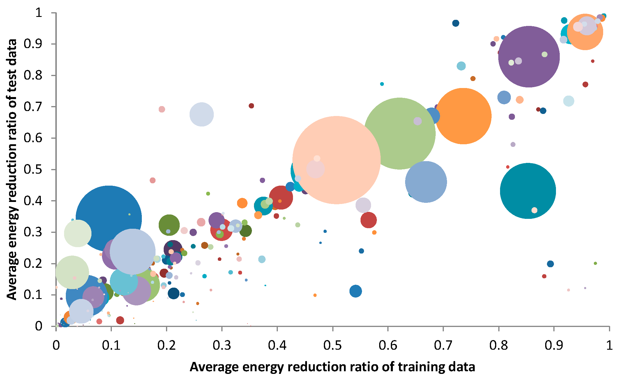
Figure 5.
Distribution of the energy reduction ratio of a customer. The energy reduction is highly dependent on the decision of the site operator. In this case, the distribution is close to bimodal distribution, rather than Gaussian distribution.
Figure 5.
Distribution of the energy reduction ratio of a customer. The energy reduction is highly dependent on the decision of the site operator. In this case, the distribution is close to bimodal distribution, rather than Gaussian distribution.

Figure 6.
Average profit of the proposed method with different stop conditions. The number of simulations (K) is fixed to 250. The perfect optimum point does not provide the best result in real test data, because of the over-fitting problem. A 2% gap in the stop condition can provide a better result, providing generalization ability in data driven methods. KRW refers to the currency of Korea (Korean Won).
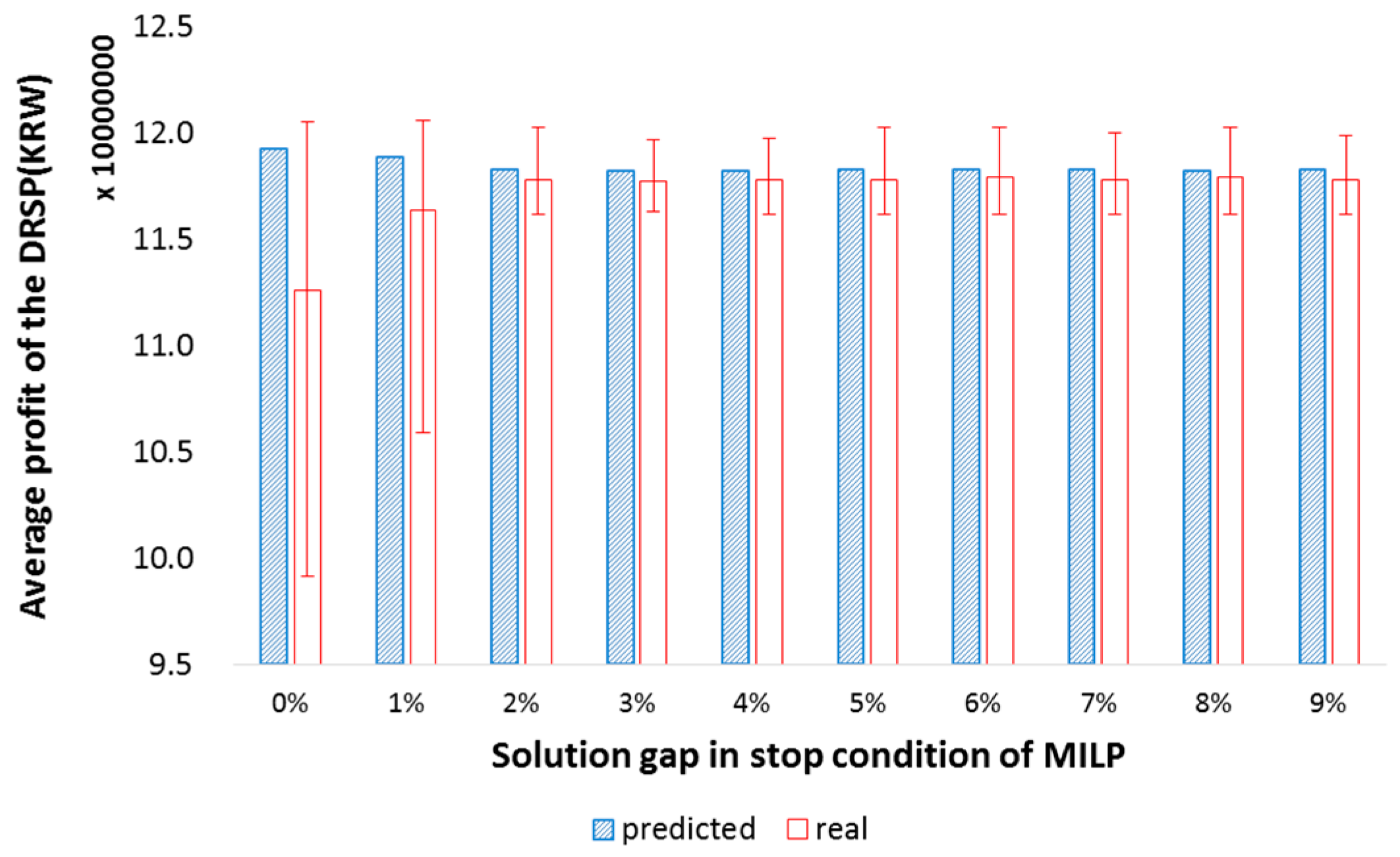
Figure 7.
Average profit of the proposed method with different numbers of samples. The stop condition is fixed to 2%. A larger number of samples tend to provide more stable results. KRW refers to the currency of Korea (Korean Won).
Figure 7.
Average profit of the proposed method with different numbers of samples. The stop condition is fixed to 2%. A larger number of samples tend to provide more stable results. KRW refers to the currency of Korea (Korean Won).

Figure 8.
Profit comparison of the proposed optimization. The real average profit of the proposed method is larger than those of all the other baselines.
Figure 8.
Profit comparison of the proposed optimization. The real average profit of the proposed method is larger than those of all the other baselines.

Figure 9.
Profit prediction error comparison. The proposed method with categorical distribution provides very low profit prediction error.
Figure 9.
Profit prediction error comparison. The proposed method with categorical distribution provides very low profit prediction error.
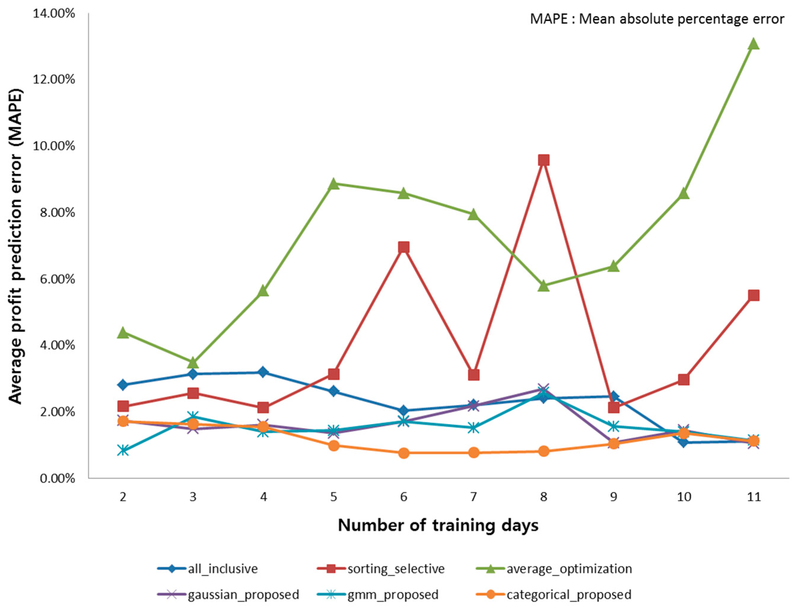
Figure 10.
Comparison of critical spread of average profit. The proposed method with categorical distribution provides very low error, and very high stability.
Figure 10.
Comparison of critical spread of average profit. The proposed method with categorical distribution provides very low error, and very high stability.
© 2017 by the authors. Licensee MDPI, Basel, Switzerland. This article is an open access article distributed under the terms and conditions of the Creative Commons Attribution (CC BY) license (http://creativecommons.org/licenses/by/4.0/).
Share and Cite
MDPI and ACS Style
Kang, J.; Lee, J.-H. Data-Driven Optimization of Incentive-based Demand Response System with Uncertain Responses of Customers. Energies 2017, 10, 1537. https://doi.org/10.3390/en10101537
AMA Style
Kang J, Lee J-H. Data-Driven Optimization of Incentive-based Demand Response System with Uncertain Responses of Customers. Energies. 2017; 10(10):1537. https://doi.org/10.3390/en10101537
Chicago/Turabian StyleKang, Jimyung, and Jee-Hyong Lee. 2017. "Data-Driven Optimization of Incentive-based Demand Response System with Uncertain Responses of Customers" Energies 10, no. 10: 1537. https://doi.org/10.3390/en10101537
Note that from the first issue of 2016, this journal uses article numbers instead of page numbers. See further details here.