The Impact of Environmental Regulation on Total Factor Energy Efficiency: A Cross-Region Analysis in China

Abstract

Environmental regulations are the key measure by which governments achieve sustainable environmental and economic development. This study aimed to determine the direct and indirect impacts of environmental regulations on total factor energy efficiency of regions in China. Since regions have different levels of economic development and resource endowment, we used the slacks-based measure (SBM)-undesirable model to calculate total factor energy efficiency considering regional technology heterogeneity and examined the regional impacts of environmental regulation on this efficiency using the Tobit regression model. A positive direct impact was generated in the eastern region of China by the forced mechanism, which forced enterprises to reduce fossil fuel energy demand and increase clean energy consumption; whereas a negative direct impact was generated in the middle and western regions owing to the green paradox, which is the observation that expected stringent environmental regulation prompts energy owners to accelerate resource extraction. Moreover, indirect impacts through technological progress and foreign direct investment were taken into account in the model, and the results show that the indirect impacts vary across regions. A logical response to these findings would be to develop different policies for different regions.

1. Introduction

Since its reform and opening up to the outside world, China has been in the process of accelerating industrialization and urbanization, and it has achieved remarkable results. However, it is undeniable that this kind of high-speed growth is based on high energy consumption. China’s energy consumption increased from 571,440,000 tons of standard coal in 1978 to 4,300,000,000 tons of standard coal in 2015, which has had huge environmental consequences. This extensive economic growth not only deteriorates the environment, but also restricts future sustainable development of China’s economy and society. As the world’s largest consumer of energy, it is imperative for China to implement an energy efficiency strategy to meet the needs of its own development and the requirements of the international community. Thus, determining how China’s environmental regulation affects its energy efficiency and exploring a balanced development model of energy efficiency improvement and environmental protection have both abstract and practical implications.

Research on energy efficiency can be divided into two categories. Earlier literature focused on single factor energy efficiency, such as unit GDP energy consumption [1,2] or energy intensity [3,4]. Single factor energy efficiency is easy to understand and convenient to calculate, but it has many problems. For example, unit GDP energy consumption cannot reflect the energy efficiency differences among different industries. In addition, these kinds of indicators ignore the substitution effect of capital, labor, and other production factors on energy input. In view of these shortcomings, the study of the concept and index of total factor energy efficiency (TFEE) emerged [5]. The TFEE concept proposed by Hu & Wang [6] is defined as the ratio of target energy input to actual input when other factors remain unchanged under the best production practice. It can be measured by different methods, one of which is the parameter method, represented by stochastic frontier analysis (SFA) [7,8], and the other is the nonparameter method, represented by data envelope analysis (DEA) [9,10]. Throughout the empirical literature on the two types of methods, empirical studies using the DEA method account for the majority of studies [11,12]; and only a few have used SFA method to calculate TFEE.

The key to using the DEA method is the selection of inputs and outputs. Traditional DEA models are assumed to be a set of outputs, and the inputs and outputs have strong disposability. Producers expect outputs to be beneficial; however, the actual production process may have undesirable outputs. These undesirable outputs must be minimized to achieve the highest economic efficiency, but the traditional DEA method can only increase them, which is contrary to the original intention of efficiency evaluation. To use the DEA method to measure economic efficiency with undesirable outputs, some scholars have extended or altered methodology. Pittman et al. [13] dealt with undesirable outputs as shadow prices. Fare et al. [14] proposed a non-linear programming approach for addressing pollution variables using the concept of weak disposability, but the non-linear programming is extremely inconvenient to use. Hailu & Veeman [15] treated undesirable outputs as inputs, which minimized the undesirable outputs but was not consistent with the actual production process. Seiford & Zhu [16] multiplied the undesirable outputs by −1 and then searched for the appropriate transition vector to convert the negative undesirable outputs to positive values. This method added a strong convexity constraint, so it can only be solved in the case of variable returns to scale. Once the constraint is canceled, the linear programming may be unsolvable. Fare et al. [17] later proposed a directional distance function from the output angle, which solved the problems of efficiency evaluation with undesirable outputs. However, this method still belonged to the radial and output angle measurement in DEA models, without fully considering the relaxation of inputs and outputs. Consequently, Tone [18,19] proposed a non-radial and non-oriented slacks-based measure (SBM) approach to solve this problem. Compared with the traditional DEA model, the SBM model directly puts slack variables into the objective function, which addresses the problems of undesirable outputs and relaxation at the same time. In addition, the SBM model can avoid the deviation of different radial and angle selections and is more effective than other models.

Due to the presence of negative externalities, greenhouse gases and toxic pollutants generated during energy use can lead to deterioration of environmental quality, a phenomenon caused mainly by market failure. According to the Coase theorem [20], governments must formulate corresponding policies and measures to mediate the interests of stakeholders in order to achieve coordinated development of environment and economy [21]. Theoretical studies have shown that environmental regulation by governments can influence the performance of enterprises, but the type of impact is debated. On one hand, environmental regulations force companies to pay a portion of the funds needed for controlling pollutants, resulting in increased production costs and consequently reduced production efficiency. On the other hand, reasonable environmental regulation produces a forcing mechanism that encourages enterprises to innovate, not only to offset the negative impact of rising costs, but also to promote technological progress, thereby enhancing production efficiency. Most early scholars supported the former effect [22,23], but recent studies have supported the latter [24,25].

Just how environmental regulation affects TFEE is not yet clear, but researchers do agree that the effects are both direct and indirect. As energy from fossil fuels is unsustainable and the pollution caused by industrial activities has external diseconomy, the government regulates the production and business activities of manufacturers through sewage permits, administrative penalties, and emission taxes to achieve sustainable development of the environment and economy [26]. These regulatory measures increase the manufacturers’ production and environmental costs, and then reduce energy demand. Therefore, because the purpose of environmental regulation policy is to protect the environment, the expected direct effect of environmental regulation on TFEE is positive. However, good intentions do not always lead to good behavior. The green paradox [27], which originates from the dynamic response of the supply side, may also result from environmental regulation. Energy owners expect more stringent environmental regulations and so mine more energy in the short term, which leads to a decrease in current energy prices. The lower energy prices stimulate an increase in energy demand, which has a negative impact on TFEE.

Environmental regulation not only has a direct impact on TFEE through energy demand and supply, but also has an indirect impact on TFEE through technological progress and foreign direct investment. Environmental regulations have positive compensation and negative offset effects on technological progress. The positive compensation effect, known as the “Porter hypothesis” effect [28], refers to the fact that appropriate environmental regulation can stimulate the innovation compensation effect. Thus, regulation can not only make up for an enterprise’s compliance costs, but can also improve its productivity and competitiveness. Therefore, environmental regulation encourages the upgrading of production technology and environmental protection technology, thereby enhancing TFEE. However, environmental regulation may increase pollution control costs, which can restrict research and development investment, a situation not conducive to environmental technology innovation. Therefore, regulation also has a negative effect on TFEE: the “compliance cost” effect [29]. In addition, Saunders [30] formally proposed the concept of the “rebound effect”, based on the research of Khazzoom [31] and Brookes [32]. The meaning of this effect is that technological progress can improve energy efficiency and reduce energy consumption, but that technological progress can also contribute to economic growth and create new demand for energy, partially or even completely offsetting the energy savings. This rebound effect cannot be negligible in empirical analysis.

Environmental regulation affects the technology spillover effect, absorptive capacity, and capital accumulation effect of foreign direct investment [33]. It increases the cost of foreign-funded enterprises and restricts research and development investment, neither of which is conducive to the spread of advanced technology. Secondly, domestic enterprises need strong learning ability and absorptive capacity to take advantage of foreign technology spillovers. Environmental regulation increases pollution control costs, thus weakening the absorptive capacity. Finally, because environmental regulation affects the choice of foreign direct investment location, stringent environmental regulation hinders the inflow of foreign direct investment, resulting in a decline in the capital stock of host countries. This is detrimental to reducing energy intensity and enhancing energy efficiency. At the same time, the impact of foreign direct investment on TFEE also plays the dual role of “angel” and “devil,” which may manifest as the “pollution aura” or “pollution heaven” [34]. As a result, environmental regulation indirectly affects TFEE. The “pollution aura” effect suggests that foreign-funded enterprises with advanced technology can spread greener and cleaner production technologies to host countries, enhancing their levels of environmental protection and thereby contributing to TFEE. To the contrary, the “pollution heaven” effect suggests that relatively liberal environmental policies and the absence of policy enforcement capacities in developing countries give them a comparative advantage in polluting-intensive industries. Developed countries may shift pollution-intensive industries to developing countries, thereby producing a negative impact on TFEE.

The region involved and the variables selected are known to influence empirical analysis on TFEE and environmental regulation, but few studies to date have acknowledged the regional differences and the indirect impact. This paper makes the following contributions to knowledge. First, considering environmental factors, undesirable outputs are incorporated into the energy efficiency calculation. Due to different levels of economic development and resource endowment, we divide China into three regions-the eastern, middle, and western-and analyze TFEE under different frontiers. Second, this paper uses the ratio of pollution control investment in GDP to measure the intensity of environmental regulation, thus taking full account of the total economic output of regions. Additionally, both the direct and indirect impacts of environmental regulation on TFEE are taken into account in the empirical analysis. Third, with respect to the disparities among different regions, we explore how the regionally different impacts of environmental regulation on TFEE promote policies targeting different regions.

The rest of this paper is organized as follows. Section 2 includes three calculation models. Section 3 describes the process of calculating TFEE and analyzes it under different frontiers. Section 4 discusses the different regional impacts of environmental regulation on TFEE, and Section 5 concludes this paper and discusses policy implications.

2. Methodology

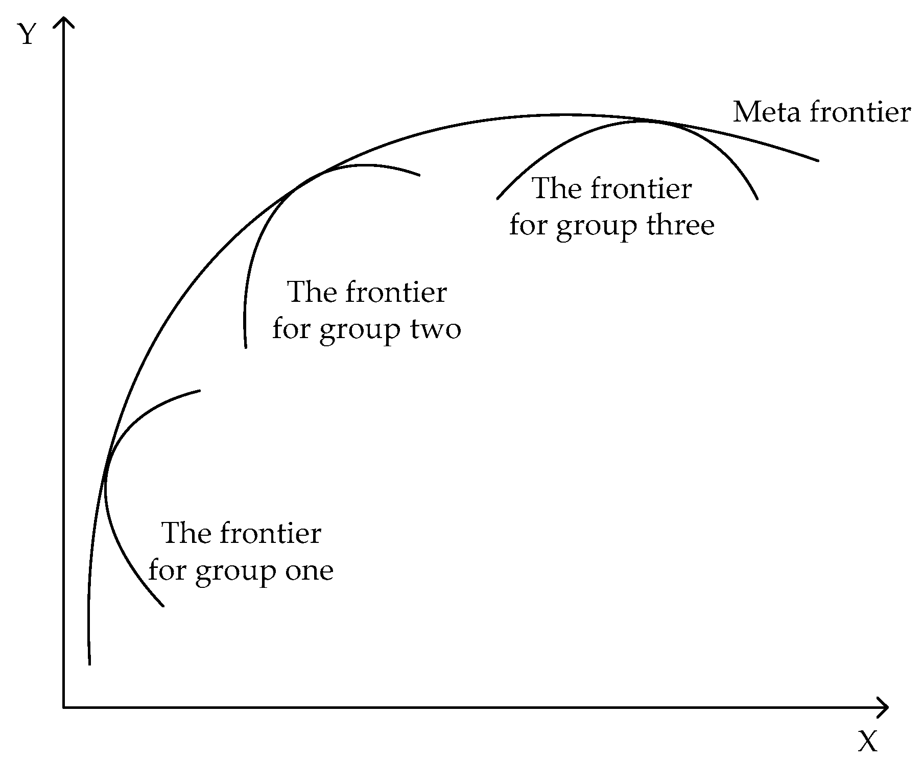
2.1. Meta-Frontier and Group Frontier Production Function

To measure the TFEE of provinces in China while considering regional technology heterogeneity, we assume that there are $n$ decision making units ($DMUs$) representing the provinces in the production system. We suppose that there are inputs $x\in R^m$, desirable outputs $y^g\in R^{s_1}$, and undesirable outputs $y^b\in R^{s_2}$ in every $DMU$, and $m$, $s_1$ and $s_2$ stand for the number of factors for inputs, desirable outputs and undesirable outputs, respectively. We define the matrices $X$, $Y^g$, and $Y^b$ as follows.

$X=\left[x_1,\cdots ,x_n\right]\in R^{m\times n}$, $Y^g=\left[y_1^g,\cdots ,y_n^g\right]\in R^{s_1\times n}$, and $Y^b=\left[y_1^b,\cdots ,y_n^b\right]\in R^{s_2\times n}$. In addition, $X>0$, $Y^g>0$, and $Y^b>0$. Notice that $x_n$ is the inputs of the n-th $DMU$; $y_n^g$ is the desirable outputs of the n-th $DMU$; $y_n^b$ is the undesirable outputs of the n-th $DMU$.

Different $DMUs$ may have different technology sets because they have varying levels of economic development and resource endowments. With this understanding, O’Donnell [35] devised the common meta-frontier and group frontier (Figure 1), and respectively defined the meta-technology ($T^{meta}$) and meta-frontier production ($P^{meta}$) possibility sets as follows.

$$T^{meta}=\left\{\left(x,y^g,y^b\right):x\mathrm{can}\mathrm{produce}\left(y^g,y^b\right)\right\},$$

(1)

$$P^{meta}=\left\{\left(x,y^g,y^b\right)|x\ge X\lambda ,y^g\le Y^g\lambda ,y^b\ge Y^b\lambda ,\lambda \ge 0\right\}$$

(2)

where $x,y^g,y^b$ are inputs, desirable outputs and undesirable outputs in $DMUs$, respectively; $T^{meta}$ indicates the specific technologies of the meta-frontier; $P^{meta}$ is the production possibility set of meta-frontier; $\lambda \in R^n$ is the intensity vector.

The meta-frontier production possibility set satisfies Brannlund et al.’s [36] regularity properties. Consequently, the meta-technology TFEE ($MTFEE$) equates to the meta-distance function ($D^{meta}$), which is defined as:

$$D^{meta}\left(x,y^g,y^b\right)={\inf }_{\theta }\left\{\theta >0:\left(\frac{y^g}{\theta }\right)\in P^{meta},\left(\frac{y^b}{\theta }\right)\in P^{meta}\right\},$$

(3)

where $\theta$ is the distance between outputs and the meta-frontier. $D^{meta}$ can be calculated using Equation (13) with the data from all groups (${\rho }^{\ast meta}$), thus:

$$MTFEE=D^{meta}\left(x,y^g,y^b\right)={\rho }^{\ast meta}.$$

(4)

The $DMU$ is efficient under the meta-production frontier when and only when ${\rho }^{\ast meta}=1$.

For the group frontier, the group technology ($T^l$) and group frontier production ($P^l$) possibility sets are defined as the following:

$$T^l=\left\{\left(x,y^g,y^b\right):x\mathrm{used}\mathrm{by}DMUs\mathrm{in}\mathrm{group}l\mathrm{can}\mathrm{produce}\left(y^g,y^b\right)\right\},$$

(5)

$$P^l=\left\{\left(x^l,y^{gl,}{y}^{bl}\right)|x^l\ge X^l\lambda ,y^{gl}\le Y^{gl}\lambda ,y^{bl}\ge Y^{bl}\lambda ,\lambda \ge 0\right\}$$

(6)

where $l=1,2,\cdots ,L$, $L$ is the number of groups classified by special standards ($L>1$) and $x^l,y^{gl},y^{bl}$ are inputs, desirable outputs, and undesirable outputs in group $l$, respectively. $T^l$ indicates the specific technologies of group $l$; $P^l$ is the production possibility set of group $l$; $\lambda \in R^n$ is the intensity vector.

Group TFEE ($GTFEE$) can be measured by the group distance function ($D^l$), which is defined as:

$$D^l\left(x,y^g,y^b\right)={\inf }_{\theta }\left\{\theta >0:\left(\frac{y^g}{\theta }\right)\in P^l,\left(\frac{y^b}{\theta }\right)\in P^l\right\},$$

(7)

where $\theta$ is the distance between outputs and the frontier of group $l$. $D^l$ can be calculated by Equation (11) with the data from group $l$ (${\rho }^{\ast l}$), thus:

$$GTFEE=D^l\left(x,y^g,y^b\right)={\rho }^{\ast l}.$$

(8)

The $DMU$ is efficient under the group production frontier when and only when ${\rho }^{\ast l}=1$.

The technology gap ratio ($TGR$) describes the gap between the group production frontier and the meta-production frontier, and is defined as

$$TGR\left(x,y^g,y^b\right)=\frac{MTFEE\left(x,y^g,y^b\right)}{GTFEE\left(x,y^g,y^b\right)}=\frac{{\rho }^{meta}}{{\rho }^l}$$

(9)

Because $D^l(x,y)\ge D^{meta}(x,y)$, $0\le TGR(x,y)\le 1$, the group production technology grows closer to the potential optimal level as the $TGR$ becomes larger, and vice versa.

The average $MTFEE$ of the l-th group ($MTFE{E}^l$) is defined as

$$MTFE{E}^l=\frac{{\displaystyle {\sum }_{i=1}^{L^l}MTFE{E}_i^l}}{L^l}$$

(10)

The average $GTFEE$ of the l-th group ($GTFE{E}^l$) is defined as

$$GTFE{E}^l=\frac{{\displaystyle {\sum }_{i=1}^{L^l}GTFE{E}_i^l}}{L^l}$$

(11)

The average meta-technology ratio of the l-th group ($TG{R}^l$) is defined as

$$TG{R}^l=\frac{{\displaystyle {\sum }_{i=1}^{L^l}TG{R}_i^l}}{L^l}$$

(12)

In the equations above, $L^l$ is the number of $DMUs$ in group $l$, $MTFE{E}_i^l$ is the $MTFEE$ of the i-th $DMU$ in group $l$, $GTFE{E}_i^l$ is the $GTE$ of the $i\mathrm{th}$ $DMU$ in group $l$, and $TG{R}_i^l$ is $TGR$ of the $i\mathrm{th}$ $DMU$ in group $l$.

2.2. SBM-Undesirable Model

A variety of DEA models are available for solving the meta-frontier and group frontier production function. The traditional DEA model needs to be modified if undesirable outputs are included. Tone [18] proposed the non-radial and non-oriented SBM approach to calculate the efficiency. In keeping with the constant returns to scale condition of this definition, the SBM has been adapted thus [19]:

$${\rho }^{*}=\min \frac{1-\frac{1}{m}{\displaystyle {\sum }_{i=1}^m\frac{s_i^{-}}{x_i}}}{1+\frac{1}{s_1+s_2}\left({\displaystyle {\sum }_{r=1}^{s_1}}\frac{s_r^g}{y_r^g}+{\displaystyle {\sum }_{r=1}^{s_2}\frac{s_r^b}{y_r^b}}\right)}$$

(13)

Subject to

$$x=X\lambda +s^{-}$$

(14)

$$y^g=Y^g\lambda -s^g$$

(15)

$$y^b=Y^b\lambda +s^b$$

(16)

$$s^{-}\ge 0, s^g\ge 0, s^b\ge 0, \lambda \ge 0$$

(17)

where $s^{-}\in R^m$ and $s^b\in R^{s_2}$ correspond to excesses of inputs and bad outputs, and $s^g\in R^{s_1}$ expresses shortages of good outputs. Let an optimal solution of the above program be $\left({\lambda }^{*},s^{-\ast },s^{g\ast },s^{b\ast }\right)$. Then, we have: the $DMU$ is efficient if and only if ${\rho }^{*}=1$, i.e., $s^{-\ast }=0$, $s^{g\ast }=0$, and $s^{b\ast }=0$. The $DMU$ is inefficient if ${\rho }^{*}<1$, and it can reach the production frontier by decreasing inputs, increasing desirable outputs, and reducing undesirable outputs.

2.3. Tobit Regression Model

Multivariate analysis models can be used to determine to what degree China’s TFEE is affected by environmental regulation. As mentioned, TFEE is generally left-censored at zero and right-censored at one. The Tobit regression model, first proposed by James Tobin [37], is a convenient method for calculating censored data [38]. The principle of maximum likelihood estimation is used to get the consistent parameter estimation. The Tobit panel regression model for evaluating the impact of China’s environmental regulation on TFEE is as follows:

$$TFE{E}_{it}^{*}={\beta }_0+{\displaystyle \sum {\alpha }_i{Z}_{it}+{\epsilon }_{it}}\sim N(0,{\sigma }^2),i=1,2,\cdots ,n,$$

(18)

$$TFE{E}_{it}=\{\begin{array}{l}TFE{E}_{it}^{*}, if <TFE{E}_{it}\le 1\\ 0,\hspace{1em}if TFE{E}_{it}>1\\ 0,\hspace{1em}if TFE{E}_{it}<0\end{array}$$

(19)

where $i$ represents for the i-th $DMU$, $t$ stands for the year, $TFE{E}_{it}^{*}$ is a latent (i.e., unobservable) variable, $Z_{it}$ is the matrix that stands for independent variables, ${\epsilon }_{it}$ is the stochastic error and submits to $N(0,{\sigma }^2)$.

3. Total Factor Energy Efficiency

3.1. Sample, Variables, and Data

In this paper, we focus on the TFEE of 30 provinces, municipalities, and autonomous regions in China during 2006 to 2015. Due to a lack of data, Tibet, Hong Kong, Macao, and Taiwan were not included. A total of 300 samples are divided into three groups, eastern, middle, and western regions, to evaluate the differences of TFEE under different technical levels. The eastern region has gentle terrain and superior geographical position, and plays the leading role in the entire economic development. The middle region is located in the inland with rich energy resources, and has a good foundation of heavy industry. The western region is vast in territory and complex in topography. Economic development level of this region is backward; however, it has great potential for development because of rich mineral resources. The numbers of samples in the eastern, middle, and western regions are 110, 80, and 110, respectively. The groupings of China’s provinces are shown in

Table 1. Groupings of China’s provinces.

Eastern Region (i = 1)		Middle Region (i = 2)		Western Region (i = 3)
j	Provinces	j	Provinces	j	Provinces
1	Beijing	1	Shanxi	1	Neimenggu
2	Tianjin	2	Jilin	2	Guangxi
3	Hebei	3	Heilongjiang	3	Chongqing
4	Liaoning	4	Anhui	4	Sichuang
5	Shanghai	5	Jiangxi	5	Guizhou
6	Jiangsu	6	Henan	6	Yunnan
7	Zhejiang	7	Hubei	7	Shanxi
8	Fujian	8	Hunan	8	Gansu
9	Shandong			9	Qinghai
10	Guangdong			10	Ningxia
11	Hainan			11	Xinjiang

.

The classic Cobb-Douglas production function takes labor and capital as inputs of production [39]. In recent years, many researchers, like Inglesi-Lotz, Papageorgiou and Reynes, regarded energy as a factor of production [40,41,42] due to the increase in energy demand. Therefore, labor, capital and energy are taken as the input factors, and real GDP is selected as the desirable output. The reason why we take SO₂ emission and chemical oxygen demand as the undesirable outputs is that they are the two most important controlling pollutants in China’s industrial system. Because the SBM-undesirable model we have chosen is used in evaluation of the $DMUs$ with multi-inputs and multi-outputs, and includes limited information of the $DMUs$. The indicators selected are not involved in all the influencing factors in regional economic activities. Other information of the $DMUs$ like their types of businesses, prices of steel and import and export of goods can also have impacts on the TFEE. The 30 provinces panel data come from the China Statistical Yearbook (2005–2016), China Energy Statistical Yearbook (2005–2016), and China Environment Yearbook (2005–2016). The descriptions of indicators for evaluating TFEE are shown in

Table 2. Indicators for evaluating total factor energy efficiency (TFEE).

Category	Variable	Unit
Inputs (x)	Labor force consumption	10,000 persons
	Capital consumption	100 million Yuan
	Energy consumption	10,000 tons of SCE
Desirable output (yg)	Gross domestic product	100 million Yuan
Undesirable outputs (yb)	SO2 emission	10,000 tons
	Chemical oxygen demand	10,000 tons

:

(1).

Labor input is represented by labor force consumption, i.e., by the average employment figure in provinces at the beginning and end of the year.

(2).

Capital input is represented by capital consumption in provinces. There is no capital stock as official data in the China Yearbooks, so we converted the capital stock data into the 2005 constant price by using Zhang et al.’s [43] perpetual inventory method.

(3).

Energy input is represented by energy consumption in standard coal units.

(4).

Desirable output is represented by the real GDP of each province, calculated as constant prices for 2005 according to the GDP deflator conversion.

(5).

Undesirable outputs contain SO₂ emissions and chemical oxygen demand, both in units of 10,000 tons.

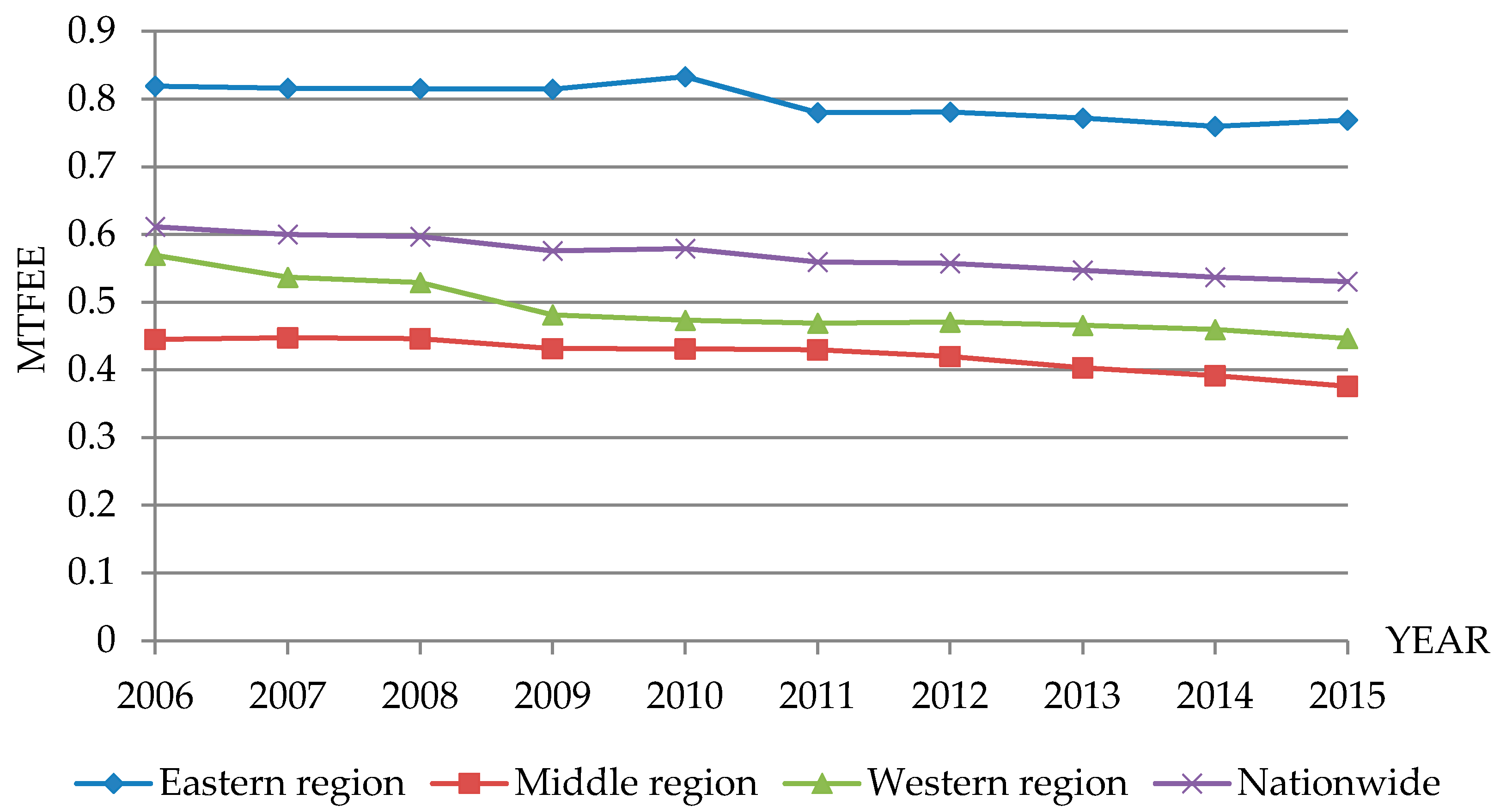
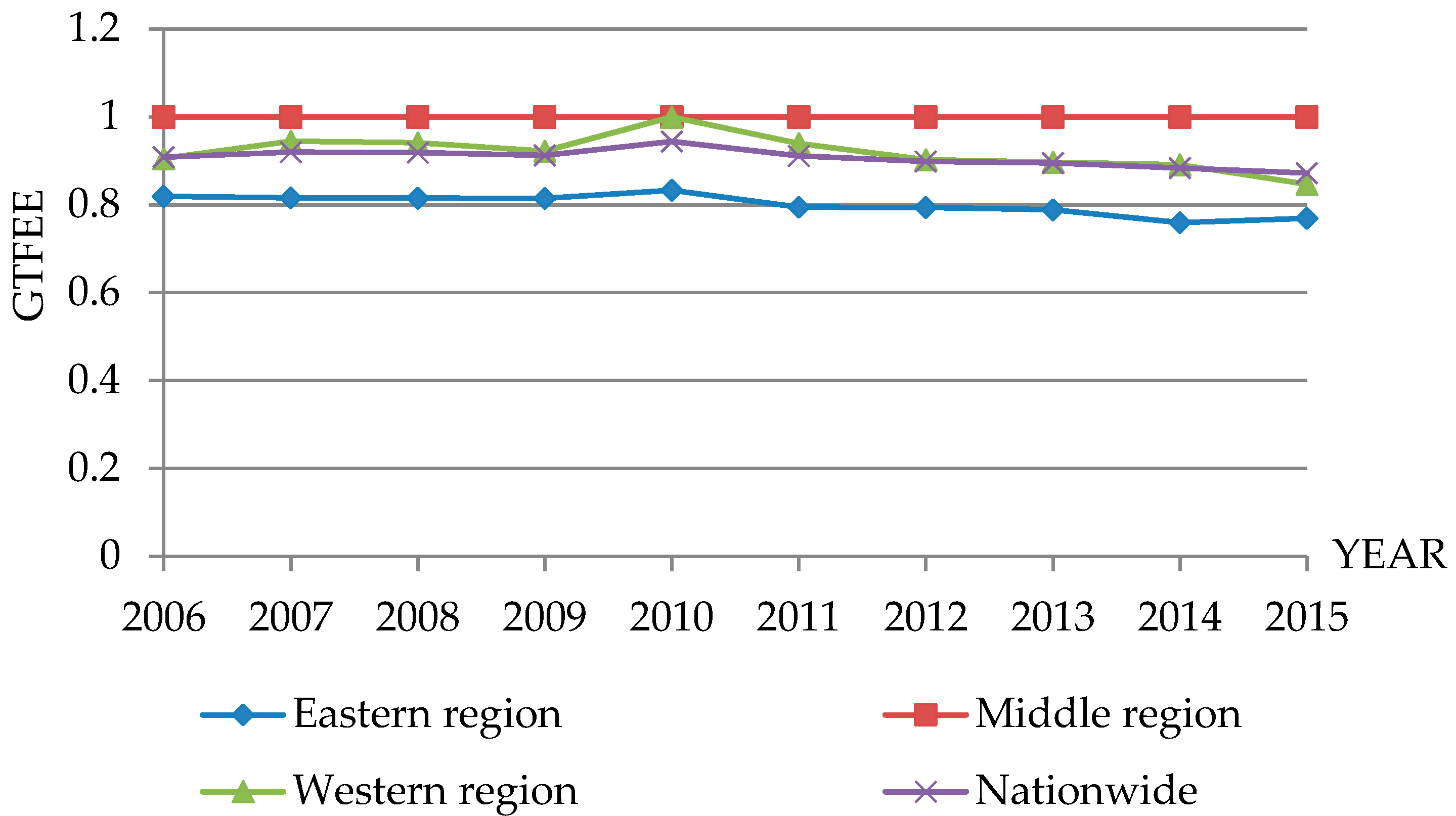
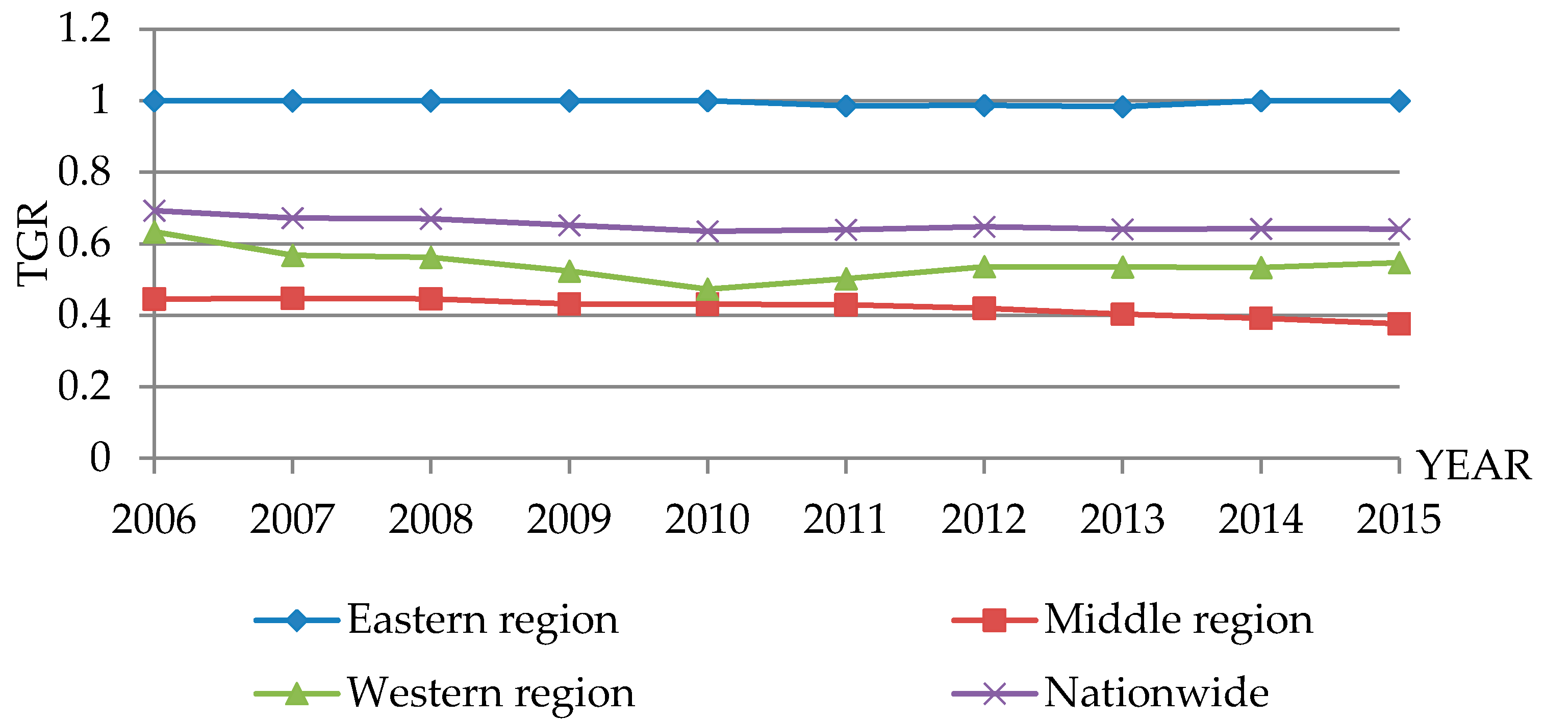
3.2. Total Factor Energy Efficiency (TFEE) under Different Frontiers

According to the Equations (1)–(8), (13) and data proposed above, this section applies STATA, which is a data analysis and statistical software, to calculate the TFEE under different frontiers from the 30 provinces in China from 2006 to 2015. The data for the average total factor efficiency of the provinces under two different frontiers is shown in

Table 3. Average TFEE of provinces under the two different frontiers.

Eastern Region	Group Frontier	Meta-Frontier	Middle Region	Group Frontier	Meta-Frontier	Western Region	Group Frontier	Meta-Frontier
Beijing	1.000	1.000	Shanxi	1.000	0.350	Neimenggu	1.000	0.388
Tianjin	1.000	0.952	Jilin	1.000	0.390	Guangxi	1.000	0.444
Hebei	0.399	0.399	Heilongjiang	1.000	0.441	Chongqing	1.000	0.443
Liaoning	0.439	0.439	Anhui	1.000	0.450	Sichuang	1.000	0.398
Shanghai	0.978	0.978	Jiangxi	1.000	0.438	Guizhou	0.836	0.364
Jiangsu	0.912	0.912	Henan	1.000	0.400	Yunnan	0.797	0.489
Zhejiang	0.750	0.750	Hubei	1.000	0.452	Shanxi	1.000	0.425
Fujian	0.549	0.549	Hunan	1.000	0.455	Gansu	0.868	0.391
Shandong	0.778	0.778				Qinghai	1.000	1.000
Guangdong	1.000	1.000				Ningxia	0.846	0.664
Hainan	1.000	1.000				Xinjiang	0.764	0.385
Average	0.800	0.796		1.000	0.422		0.919	0.490

and the $TGR$ is shown in

Table 4. Average technology gap ratio (TGR) of provinces.

Eastern Region	TGR	Middle Region	TGR	Western Region	TGR
Beijing	1.000	Shanxi	0.350	Neimenggu	0.388
Tianjin	0.952	Jilin	0.390	Guangxi	0.444
Hebei	1.000	Heilongjiang	0.441	Chongqing	0.443
Liaoning	1.000	Anhui	0.450	Sichuang	0.398
Shanghai	1.000	Jiangxi	0.438	Guizhou	0.459
Jiangsu	1.000	Henan	0.400	Yunnan	0.599
Zhejiang	1.000	Hubei	0.452	Shanxi	0.425
Fujian	1.000	Hunan	0.455	Gansu	0.464
Shandong	1.000			Qinghai	1.000
Guangdong	1.000			Ningxia	0.804
Hainan	1.000			Xinjiang	0.531
Average	0.996		0.422		0.541

.

Under the group frontier, from 2006 to 2015, the average total factor energy efficiencies of the three regions are 0.800, 1.000, and 0.919, respectively. The middle region is the best performer, and the eastern region is the worst. The average values imply that the three regions can improve TFEE by 20%, 0, and 8.1%, respectively, if all within-region provinces practice on the group frontier. In the eastern region, TFEE of the provinces ranges from 0.399 to 1.000. Four of the provinces, Beijing, Tianjin, Guangdong, and Hainan, reach the frontier. However, Hebei, Liaoning, Fujian, Zhejiang, and Shandong perform worse, with values below the average level of the eastern region. Particularly, Hebei Province has the lowest value due to its unreasonable energy usage and severe contamination [44]. One the other hand, Hebei Province has the greatest potential to improve its energy usage level. In the middle region, the TFEE of all provinces operates on the boundary of the group frontier, thus indicating that the middle region has no potential to improve its TFEE. In the western region, TFEE of the provinces ranges from 0.764 to 0.868. More than half of the provinces in the western region have reached the group frontier, including Neimenggu, Guangxi, Chongqing, Sichuang, Shanxi, and Qinghai. The remaining provinces perform better as their TFEE is not much lower than the unit value.

Under the meta-frontier, from 2006 to 2015, the average total factor energy efficiencies of the three regions are 0.796, 0.422, and 0.490, respectively. The eastern region performs much better than the middle and western regions. The average values mean that if all provinces in China practice best on the meta-frontier, the three regions can improve their TFEE by 20.4%, 57.8%, and 51.0%, respectively. In the eastern region, the TFEE of provinces also ranges, from 0.399 to 1.000. Three provinces, Beijing, Guangdong, and Hainan, reach the unit value. Compared to the condition of the group frontier, the TFEE of Tianjin changes, from 1 to 0.952, indicating that Tianjin has the potential to improve its TFEE by 4.8%. The middle region has the worst performance under the meta-frontier. In the middle region, the TFEE of each province is below 0.500, significantly lower than the value under the group frontier. Although these provinces behave best under the group frontier, they still have a big gap compared with the provinces in other regions. Hunan, Hubei, Anhui, Heilongjiang, and Jiangxi perform better than the average level. Shanxi has the worst performance, with a value of 0.350. In the western region, the TFEE is significantly lower than the value under the group frontier. Only one province, Qinghai, reaches the meta-frontier, and more than half of the provinces perform worse than the average level. Only the results for Qinghai and Ningxia, are better than the average level; their TFEE is greater than that of other provinces in the western region.

We calculate the technology gap ratio (TGR) according to Equations (1)–(13). The average TGR values of the three regions are 0.996, 0.422, and 0.541, respectively, which are less than 1. The results indicate that TFEE gaps between the group production frontier and the meta-production frontier exist. Only the eastern region has a TGR value close to 1, which means that energy use in this region is relatively reasonable. This value is a result of advanced energy-use technology. The middle and western regions are significantly behind the eastern region in TGR. A large TFEE gap exists between the group production frontier and the meta-production frontier in these two regions. In the middle region, the TGR value of each province is below 0.5, because the provinces in this region do not have advanced energy-use technology. In the western region, although the average value of TGR is not high, two provinces, Qinghai and Ningxia, have relatively high TGRs, which are much higher than those of the other provinces. In summary, levels of energy use technology among the regions are imbalanced. The eastern region has gradually developed advanced technology in the process of economic development. As energy output regions and industry receiving regions, the middle and western regions have been facing the “resource curse” problem [45] and have not improved the level of energy use technology.

The above 30 provinces are divided into three regions. As shown in Figure 2, the total factor efficiency of the eastern region under the meta-frontier has the highest level, higher than the national average. The western region is second, and slightly lower than the national average. The middle region has the worst performance, which is significantly lower than the performance of both the eastern region and the national average. The TFEE under the meta-frontier has decreased slowly over the years, which is not a positive trend as the level of energy use in each region has not improved over time. Setting a period of five years as a timeframe, the TFEE under the meta-frontier of the eastern region increased steadily in the first five years, reached a peak in 2010, but then decreased quickly. The middle region showed a considerable decrease over the first five years, and then continued to decrease gradually. The western region showed fluctuating values over the first five years, but values decreased in the second five years. Overall, the TFEE under the meta-frontier of the regions during the Eleventh Five-Year Plan is better than that during the Twelfth Five-Year Plan. This downward trend does not match with China’s rapid macroeconomic growth during these ten years.

As shown in Figure 3, the total factor efficiency of the middle region under the group frontier is the highest, slightly higher than the national average. The western region has the second highest level similar to the national average. The eastern region ranks last and stands apart from the middle region, western region, and the national average. The TFEE under the group frontier generally remained stable over the years. The results show rapid growth from 2009 to 2010, with a peak and also a turning point occurring in 2010. Since that year, the TFEE has remained steady. Over the years, the TFEE for almost all of the regions was between 0.8 and 1. In each region, the performance of the provinces was steady and close to the group technology boundary. Overall, during the ten years, there was not much change of the TFEE of the regions under the group frontier. The performance of regions during the Twelfth Five-Year Plan is no better than that during the Eleventh Five-Year Plan. Economic development over time did not result in an improvement of TFEE under the group frontier.

The different regions have different technical gaps due to the unbalanced levels of economic development. As shown in Figure 4, the eastern region TGR ranks first, with values significantly higher than the national average and the western and middle regions. It is very steady and close to 1, which means that the eastern region has had stable and advanced energy-use technology over the two five-year plans. The western region TGR has the second highest level, slightly lower than the national average. It decreased obviously during the Eleventh Five-Year Plan and reached its lowest point in 2010. During these five years, the technology gap between the group production frontier and the meta-production frontier of the western region expanded gradually. The technology level gap between the western region and the eastern region also expanded through this time. During the Twelfth Five-Year Plan, the western region TGR increased slightly, but did not reach the previous highest point. Although the gap between the group production frontier and the meta-production frontier of the western region narrowed gradually, the level of advanced technology had not been improved. Among all the regions, the TGR of the middle region had the lowest level during the past ten years. This indicates that the middle region had the largest gap between the group production frontier and the meta-production frontier and therefore that the middle region had the most backward technical level among these three regions.

4. Empirical Analysis

4.1. Selection of Influencing Factors

In studies of environmental regulation (ER), scholars have identified three relevant indicators, which are mainly as follows [46,47,48]: (1) the number of policies and regulations promulgated by regulatory agencies; (2) the compliance rate of pollutant discharge under regulation; and (3) the pollution control expenditure. We are more inclined to use pollution control expenditure to measure the intensity of environmental regulation because pollution control expenditure is positively related to the intensity of environmental regulation and the investment in pollution control in the provinces is available. In the actual calculation, we use the ratio of pollution control investment in GDP to measure the intensity of environmental regulation. This approach takes full account of the total economic output of the regions and provinces, and thus is more consistent with theoretical logic. Compared with other regions and provinces, a relatively smaller pollution control investment cannot directly explain why the region’s or province’s environmental regulation is looser. However, the difference may be due to the region’s or province’s smaller total economic scale. Therefore, it is more reasonable to use the pollution control investment of per unit output to measure the intensity of environmental regulation.

Many factors influence energy efficiency. To improve the breadth of our research, and according to the existing research and data availability, we added selected factors to the model to act as control variables. These indices, used in the empirical analysis, are industrial structure ($IS$), technological progress ($TP$), energy structure ($ES$), and opening degree ($OD$). Industrial structure is the proportion of GDP attributable to secondary industry. The demands for energy differ among industries, and secondary industry, especially heavy industry, has a relatively high demand for energy. Technological progress is represented by the proportion of the GDP devoted to intramural expenditures on research and development. On one hand, through the improvement and replacement of technology and equipment, technological innovation will improve energy efficiency to a certain extent. On the other hand, in the process of technological progress, a rebound effect exists, which increases the demand for energy. Energy structure is the proportion of coal consumption within the total energy consumption. In China, the traditional energy consumption structure depends mainly on coal, which is not helpful to the improvement of TFEE. The opening degree is represented by the proportion of GDP that is foreign direct investment. The pollution haven hypothesis suggests that countries with lower environmental standards or weaker enforcement easily attract investment from foreign countries. However, the introduction and use of foreign capital may be conductive to improving TFEE because advanced energy-use technology is introduced at the same time.

We made the orders of magnitude consistent and eliminated the exponential growth trend of several variables by calculating the original variables’ logarithm, $lnER$, $lnIS$, $lnTP$, $lnES$, and $lnOD$. The panel data for the 30 provinces are taken from the China Statistical Yearbook (2005–2016), China Energy Statistical Yearbook (2005–2016), and China Statistical Yearbook on Science and Technology (2005–2016).

4.2. Empirical Results and Analysis

As discussed previously, we used the Tobit model for the empirical analysis of the impact of environmental regulation on TFEE. The empirical analysis created the cross item “environmental regulation and technological progress”, as the government’s regulation policy produces an incentive effect on progress in energy-saving and emissions-reduction technology. Enterprises have to consider additional restrictions due to environmental regulation, which may induce technological innovation. At the same time, the cross item “environmental regulation and opening degree” was added to the function. This cross item explains the indirect effect of government regulation policy on TFEE. The strength of environmental regulation determines the level of environmental threshold. A high environmental threshold may deter foreign companies with high energy consumption and pollution from entering and attract high-quality inflows of foreign direct investment, thus preventing the region from becoming a “pollution heaven”. To investigate the different impacts of the factors on the TFEE in the different regions, this paper not only analyzes the regression at the national level but also further tests regional influences.

Table 5. Regression results of the Tobit model.

Variable	National	Eastern Region	Middle Region	Western Region
$lnER$	−0.0511 **	0.0219 **	−0.0030 **	−0.1066 **
	(−2.05)	(2.03)	(2.16)	(−2.30)
$lnIS$	−0.1691 *	0.0136 ***	−0.3128 ***	−2.459 ***
	(−1.78)	(3.03)	(-9.48)	(−3.22)
$lnTP$	−0.1269 ***	−0.2435 **	−0.0455 **	−0.2165 ***
	(−2.99)	(−2.03)	(−2.22)	(−3.31)
$lnES$	−0.4425	−0.2427	−0.0051	−0.2690
	(−0.56)	(−0.87)	(−0.07)	(−0.88)
$lnOD$	−0.0136	−0.1330 ***	0.0082	0.2226
	(−0.58)	(−3.14)	(0.66)	(1.40)
$lnER*lnTP$	0.0664 *	−0.0778 *	0.0639 **	0.6890 *
	(1.62)	(−1. 83)	(2.13)	(1.66)
$lnER*lnOD$	0.0209 *	0.2168 ***	−0.0035	−0.3847 **
	(1.91)	(3.12)	(−0.21)	(−2.03)
$cons$	1.4905 ***	2.1293	2.1372 ***	11.6877 ***
	(2.82)	(1.09)	(9.33)	(3.63)
$sigma\_u$	0.3709 ***	0.5010 ***	0.0405 ***	0.4293 **
	(5.83)	(2.67)	(3.70)	(2.02)
$sigma\_e$	0.0951 ***	0.1302 ***	0.0220 ***	0.2771 ***
	(19.50)	(8.54)	(11.93)	(5.77)
$rho$	0.9384	0.9367	0.7718	0.7059

The number in the parentheses is the z-value. *, **, *** significant at the 10%, 5%, and 1% level, respectively.

reports the result.

As shown in Table 5, the coefficient of $lnER$ in the eastern region is significantly positive, and the coefficients of $lnER$ in the whole nation, middle region, and western region are significantly negative. Thus, environmental regulations can improve TFEE in the eastern region, but that it would have an opposite effect in the other regions. In this case, eastern region can improve TFEE by 0.0219% if its environmental regulation intensity increases by 1%. This relationship between environmental regulation and TFEE in the eastern region verifies the existence of the “forced mechanism.” Environmental protection measures, such as the fossil energy tax and clean energy subsidies, have created a forced mechanism in the eastern region. The costs for enterprises in pollution abatement for end-of-pipe control have become so high that enterprises are facing declining profits and great pressure to reduce emissions. In order to maintain a competitive advantage in the market, enterprises want to reduce production costs and also reduce pollutant emissions. Because fossil fuels are a major source of pollution, enterprises have increasing momentum to reduce fossil fuel energy demand and increase clean energy consumption, which then improves energy efficiency. In addition, this forced mechanism forms market barriers to new enterprises wishing to enter the region. High pollution and energy consumption industries may increase investment for updating and gradually phasing out or move to other regions. However, the TFEE will reduce by 0.0511%, 0.0030% and 0.1066%, respectively, in the entire nation and the middle and western regions, if their environmental regulation intensities increase by 1%. This is because environmental regulation produces a green paradox on TFEE. The middle and western regions are rich in energy and mineral resources. As these regions are major suppliers of energy, the proportion of mining and raw materials industries in these regions is relatively large. Expected stringent environmental regulation prompts energy owners to exploit energy in advance, which causes high amounts of pollution in the short term and is unfavorable to the promotion of TFEE. Additionally, the increase in energy supply leads to lower energy prices and increasing demand for energy, which is not conducive to TFEE.

Environmental regulation not only has a direct impact on TFEE, but also has an indirect impact through technological progress. The coefficient of the cross item, $lnER*lnTP$, explains this indirect impact. Firstly, the coefficients of $lnTP$ are significantly negative in all regions. This result shows that technological progress without environmental regulation plays a negative role in enhancing TFEE. Technological progress without environmental regulation is directed mainly toward increasing production, rather than toward energy savings and emission reductions. This improvement of production technology can bring about a rebound effect, possibly leading to more pollution. Both higher energy input and pollution emissions have negative effects on TFEE. Secondly, when considering environmental regulation, the cross-item coefficient of “environmental regulation and technological progress” in the eastern region is significantly negative, whereas these cross-item coefficients in the middle and western regions are significantly positive. In the context of environmental regulation, enterprises will increase investment in energy-saving and emissions-reduction technology. The environmental pollution and technical infrastructure in the middle and western regions are worse than those in the eastern region. As a result, the marginal benefits from investment in energy-saving and emissions-reduction technology in the middle and western regions are higher than those in the eastern region. The indirect effect of environmental regulation on TFEE through technological progress is characterized as a compliance cost effect in the eastern region but as a Porter hypothesis effect in the middle and western regions. At the same time, the developed eastern region with advanced production technology is more likely to have a rebound effect, which may lead to higher energy input and lower energy efficiency. Therefore, in the case of environmental regulation, the cost of technological progress in the eastern region is greater than the proceeds, and an increase of 1% of technological progress investment can reduce the TFEE by 0.0778%; whereas the cost of technological progress in the nation and middle and western regions is lower than the proceeds, and an increase of 1% of technological progress investment can improve the TFEE by 0.0644%, 0.0639% and 0.6890%, respectively.

The opening degree is another important variable between environmental regulation and TFEE. Firstly, the coefficient of $lnOD$ in the eastern region is significantly negative, and the “pollution heaven” is a driver of trade flows. In contrast, the coefficients of $lnOD$ in the whole nation, middle region, and western region are positive, but the impact of opening degree on energy efficiency is not significant. The impact of opening degree on energy efficiency plays a dual role, and may result in either a positive or negative effect. In China, the eastern region has the highest opening degree among the regions. In order to maintain or enhance the competitive advantage and attractiveness of foreign investment, the government of this region has given latent super-national treatment to foreign enterprises over a long period. In regard to environmental regulation, intergovernmental competition has led to a “race to the bottom”, which can account for the eastern region’s nickname of “pollution heaven”. However, the extent to which opening degree impacts the whole nation, middle region, and western region is not clear.

The results described above are the impacts of opening degree without environmental regulation. The situation with environmental regulation is discussed below. When environmental regulation in China is “loose”, developed countries with stringent environmental regulation will move polluting industries to China. At this time, the inflow of foreign direct investment will bring a “pollution heaven” effect, which has a negative effect on TFEE. However, stringent environmental regulation has a screening effect on foreign direct investment. Industries that are conducive to environmental protection and technology upgrades are welcomed and their requests prioritized. This forms a “crowding out effect” on foreign direct investment in pollution-intensive industries, which in turn has a positive effect on TFEE. The eastern region was the first open area in China. Therefore, with continuous economic and social development, the eastern region has developed the ability to select qualified foreign direct investment. The introduction of high-quality foreign direct investment, equivalent to the introduction of advanced energy-use technology, will improve its TFEE. Therefore, the cross-item coefficient of “environmental regulation and opening degree” in the eastern region is significantly positive. In the case of environmental regulation, the TFEE will increase by 0.2168% if the foreign direct investment attracted by the eastern region increases by 1%. However, the cross-item coefficient of “environmental regulation and opening degree” in the western region is significantly negative. In the case of environmental regulation, if the foreign direct investment attracted by the western region increases by 1%, the TFEE will reduce by 0.3847%. Because the natural and social environments in the western region are not good, environmental regulation weakens its capability to attract foreign direct investment. In other words, the western region has a reduced opportunity to absorb advanced energy-use technology from developed countries. In the middle region, the cross-item coefficient of environmental regulation and opening degree is negative, but not significant. It is not clear to what extent environmental regulation through opening degree impacts this region.

The effects of industrial and energy structures on the TFEE of the regions are as follows. The coefficient of $lnIS$ in the eastern region is significantly positive, and the coefficients of $lnIS$ in the whole nation, middle region, and western region are significantly negative. These different regions have different industrial layouts and levels of industrialization. The eastern region has an advanced industrialization level, and its secondary industry, with lower energy consumption, is based mainly on capital and labor. However, the middle and western regions have relatively backward industrialization levels, and their secondary industry is based mainly on resource processing. Additionally, higher energy consumption and polluting industries have transferred from the eastern region to the middle and western regions in the process of industrialization. Although the coefficient of $lnES$ is negative, the impact of energy structure on energy efficiency is not significant, which is not consistent with expectations. There is no evidence that the energy consumption structure is the main bottleneck constraining TFEE. China’s energy endowment structure, with abundant coal but scarce oil and gas resources, determines the long-term coal-based energy consumption structure. It is not realistic to attempt to improve the TFEE by changing the energy consumption structure in the short term.

5. Conclusions

As a result of measuring the TFEE and the impact of environmental regulation on it, this paper has reached the following main conclusions.

(1).

During 2006 to 2015, the overall levels of TFEE under the group frontier and the meta-frontier in China were low. Thus, great potential for improving energy efficiency exists. Throughout the regions in China, TFEE is significantly imbalanced.

(2).

Environmental regulations have not only direct but also indirect effects on TFEE through technological progress and opening degree. Because of the different levels of economic and social development, how environmental regulations impact TFEE varies from region to region.

In the eastern region, the direct impact of environmental regulation on TFEE verifies the existence of the forced mechanism of environmental regulation, which can improve TFEE. However, the indirect impact of environmental regulation on TFEE through technological progress is negative. Additionally, environmental regulation increases the threshold of foreign direct investment to the eastern region, which is beneficial to improving its TFEE.

In the middle and western regions, the direct impact of environmental regulation on TFEE is consistent with the green paradox. Environmental regulation becomes a factor in increasing energy demand and has a negative impact on TFEE. However, the indirect effect verifies the Porter hypothesis and has a positive impact on TFEE. Nevertheless, in the western region, environmental regulation weakens the ability to attract foreign direct investment, thereby reducing access to advanced energy utilization technologies and producing a negative impact on the area’s TFEE.

6. Future Policy Recommendation

According to the above discussion and conclusions, we recommend the following:

(1).

Implementing regional differentiated environmental regulation policies: Due to the regional differences in development, China should implement differentiated environmental regulation policies in accordance with the environmental and economic responsibilities of the different regions. In the eastern region, a relatively stringent environmental regulation policy should be implemented, whereas in the middle and western regions, the enterprise access mechanism can be appropriately relaxed on the basis of full consideration of the environmental carrying capacity.

(2).

Increasing investment in innovation of energy-saving and emissions-reduction technology: Investment in technological innovation should focus on promoting the development and application of energy-saving and emissions-reduction technology. Increased investment will encourage enterprises to innovate technology, purchase advanced equipment, and introduce foreign advanced energy-saving management practices. At the same time, the government needs to rein in the rebound effect through leverage such as an energy tax.

(3).

Constructing a regional compensation mechanism for environmental protection: In the process of implementing environmental regulation, the cost of regional environmental protection should be allocated rationally. When accepting industrial transfers or foreign direct investment, all regions should agree on the compensation mechanism for environmental protection according to the polluter pays principle. For the poverty-stricken and ecologically fragile areas in the middle and western regions, the government should strengthen its planning and guidance to encourage the full provision of regional environmental public goods and thus gradually promote TFEE.

References

1. Soytas, U.; Sari, R. Energy consumption and gdp: Causality relationship in g-7 countries and emerging markets. Energy Econ. 2003, 25, 33–37. [Google Scholar] [CrossRef]
2. Crompton, P.; Wu, Y. Energy consumption in China: Past trends and future directions. Energy Econ. 2005, 27, 195–208. [Google Scholar] [CrossRef]
3. Fisher-Vanden, K.; Jefferson, G.H.; Liu, H.; Tao, Q. What is driving China’s decline in energy intensity? Resour. Energy Econ. 2004, 26, 77–97. [Google Scholar] [CrossRef]
4. Sinton, J.E.; Levine, M.D. Changing energy intensity in Chinese industry: The relatively importance of structural shift and intensity change. Energy Policy 1994, 22, 239–255. [Google Scholar] [CrossRef]
5. Chang, M.-C. A comment on the calculation of the total-factor energy efficiency (TFEE) index. Energy Policy 2013, 53, 500–504. [Google Scholar] [CrossRef]
6. Hu, J.-L.; Wang, S.-C. Total-factor energy efficiency of regions in China. Energy Policy 2006, 34, 3206–3217. [Google Scholar] [CrossRef]
7. Aigner, D.; Lovell, C.K.; Schmidt, P. Formulation and estimation of stochastic frontier production function models. J. Econ. 1977, 6, 21–37. [Google Scholar] [CrossRef]
8. Battese, G.E.; Coelli, T.J. A model for technical inefficiency effects in a stochastic frontier production function for panel data. Empir. Econ. 1995, 20, 325–332. [Google Scholar] [CrossRef]
9. Seiford, L.M.; Thrall, R.M. Recent developments in dea: The mathematical programming approach to frontier analysis. J. Econ. 1990, 46, 7–38. [Google Scholar] [CrossRef]
10. Cook, W.D. Data envelopment analysis: A comprehensive text with models, applications, references and dea-solver software. JSTOR 2001, 31, 116–118. [Google Scholar]
11. Zhou, P.; Poh, K.L.; Ang, B.W. Data envelopment analysis for measuring environmental performance. In Handbook of Operations Analytics Using Data Envelopment Analysis; Springer: Berlin, Germany, 2016; pp. 31–49. [Google Scholar]
12. Babazadeh, R.; Razmi, J.; Rabbani, M.; Pishvaee, M.S. An integrated data envelopment analysis–mathematical programming approach to strategic biodiesel supply chain network design problem. J. Clean. Prod. 2017, 147, 694–707. [Google Scholar] [CrossRef]
13. Pittman, R.W. Multilateral productivity comparisons with undesirable outputs. Econ. J. 1983, 93, 883–891. [Google Scholar] [CrossRef]
14. Färe, R.; Grosskopf, S.; Lovell, C.K.; Pasurka, C. Multilateral productivity comparisons when some outputs are undesirable: A nonparametric approach. Rev. Econ. Stat. 1989, 71, 90–98. [Google Scholar] [CrossRef]
15. Hailu, A.; Veeman, T.S. Non-parametric productivity analysis with undesirable outputs: An application to the canadian pulp and paper industry. Am. J. Agric. Econ. 2001, 83, 605–616. [Google Scholar] [CrossRef]
16. Seiford, L.M.; Zhu, J. Modeling undesirable factors in efficiency evaluation. Eur. J. Oper. Res. 2002, 142, 16–20. [Google Scholar] [CrossRef]
17. Färe, R.; Grosskopf, S. Nonparametric productivity analysis with undesirable outputs: Comment. Am. J. Agric. Econ. 2003, 85, 1070–1074. [Google Scholar] [CrossRef]
18. Tone, K. A slacks-based measure of efficiency in data envelopment analysis. Eur. J. Oper. Res. 2001, 130, 498–509. [Google Scholar] [CrossRef]
19. Tone, K. Dealing with Undesirable Outputs in Dea: A Slacks-Based Measure (SBM) Approach; GRIPS Research Report Series; National Graduate Institute for Policy Studies: Tokyo, Japan, 2003. [Google Scholar]
20. Cooter, R.D. The coase theorem. In Allocation, Information and Markets; Springer: Berlin, Germany, 1989; pp. 64–70. [Google Scholar]
21. Bel, G.; Costas, A. Do public sector reforms get rusty? Local privatization in Spain. J. Policy Reform 2006, 9, 1–24. [Google Scholar] [CrossRef]
22. Jorgenson, D.W.; Wilcoxen, P.J. Environmental regulation and us economic growth. Rand J. Econ. 1990, 21, 314–340. [Google Scholar] [CrossRef]
23. Barbera, A.J.; McConnell, V.D. The impact of environmental regulations on industry productivity: Direct and indirect effects. J. Environ. Econ. Manag. 1990, 18, 50–65. [Google Scholar] [CrossRef]
24. Qinghuang, H.; Ming, G. A research on the energy conservation and emission reduction effect of China’s environmental regulation tools. Sci. Res. Manag. 2016, 6, 003. [Google Scholar]
25. Zhou, X.; Feng, C. The impact of environmental regulation on fossil energy consumption in China: Direct and indirect effects. J. Clean. Prod. 2017, 142, 3174–3183. [Google Scholar] [CrossRef]
26. Zhu, Q. A perspective of evolution for carbon emissions trading market: The dilemma between market scale and government regulation. Discret. Dyn. Nat. Soc. 2017, 2017, 1432052. [Google Scholar] [CrossRef]
27. Sinn, H.-W. Public policies against global warming: A supply side approach. Int. Tax Public Financ. 2008, 15, 360–394. [Google Scholar] [CrossRef]
28. Porter, M.E. Competitive Strategy: Techniques for Analyzing Industries and Competitors; Simon and Schuster: New York, NY, USA, 2008. [Google Scholar]
29. Jaffe, A.B.; Palmer, K. Environmental regulation and innovation: A panel data study. Rev. Econ. Stat. 1997, 79, 610–619. [Google Scholar] [CrossRef]
30. Saunders, H.D. The khazzoom-brookes postulate and neoclassical growth. Energy J. 1992, 13, 131–148. [Google Scholar] [CrossRef]
31. Einhorn, M. Economic implications of mandated efficiency standards for household appliances: An extension. Energy J. 1982, 3, 103–109. [Google Scholar] [CrossRef]
32. Brookes, L. The energy price fallacy and the role of nuclear power in the UK. Energy Policy 1978, 6, 94–106. [Google Scholar] [CrossRef]
33. Zghidi, N.; Mohamed Sghaier, I.; Abida, Z. Does economic freedom enhance the impact of foreign direct investment on economic growth in north African countries? A panel data analysis. Afr. Dev. Rev. 2016, 28, 64–74. [Google Scholar] [CrossRef]
34. Boontem, K. An impact of pollution control enforcements on fdi inflow. Bus. Manag. Rev. 2016, 7, 155. [Google Scholar]
35. O’Donnell, C.J.; Rao, D.P.; Battese, G.E. Metafrontier frameworks for the study of firm-level efficiencies and technology ratios. Empir. Econ. 2008, 34, 231–255. [Google Scholar] [CrossRef]
36. Brännlund, R.; Färe, R.; Grosskopf, S. Environmental regulation and profitability: An application to Swedish pulp and paper mills. Environ. Resour. Econ. 1995, 6, 23–36. [Google Scholar] [CrossRef]
37. Tobin, J. Estimation of relationships for limited dependent variables. Econ. J. Econ. Soc. 1958, 26, 24–36. [Google Scholar] [CrossRef]
38. Anastasopoulos, P.C.; Tarko, A.P.; Mannering, F.L. Tobit analysis of vehicle accident rates on interstate highways. Accid. Anal. Prev. 2008, 40, 768–775. [Google Scholar] [CrossRef] [PubMed]
39. Cobb, C.W.; Douglas, P.H. A theory of production. Am. Econ. Rev. 1928, 18, 139–165. [Google Scholar]
40. Inglesi-Lotz, R. The impact of renewable energy consumption to economic growth: A panel data application. Energy Econ. 2016, 53, 58–63. [Google Scholar] [CrossRef]
41. Papageorgiou, C.; Saam, M.; Schulte, P. Substitution between clean and dirty energy inputs: A macroeconomic perspective. Rev. Econ. Stat. 2017, 99, 281–290. [Google Scholar] [CrossRef]
42. Reynès, F. The Cobb-Douglas Function as a Flexible Function: Analysing the Sustitution between Capital, Labor and Energy; SciencesPo: Paris, France, 2017. [Google Scholar]
43. Jun, Z.; Guiying, W.; Jipeng, Z. The estimation of China’s provincial capital stock: 1952—2000. Econ. Res. J. 2004, 10, 35–44. [Google Scholar]
44. Liu, G.; Yang, Z.; Chen, B.; Zhang, Y.; Su, M.; Ulgiati, S. Prevention and control policy analysis for energy-related regional pollution management in China. Appl. Energy 2016, 166, 292–300. [Google Scholar] [CrossRef]
45. Robinson, J.A.; Torvik, R.; Verdier, T. The political economy of public income volatility: With an application to the resource curse. J. Public Econ. 2017, 145, 243–252. [Google Scholar] [CrossRef]
46. Amir, R.; Gama, A.; Werner, K. On environmental regulation of oligopoly markets: Emission versus performance standards. Environ. Resour. Econ. 2017, 1–21. [Google Scholar] [CrossRef]
47. Demmig-Adams, B.; Stewart, J.J.; Adams, W.W. Environmental regulation of intrinsic photosynthetic capacity: An integrated view. Curr. Opin. Plant Biol. 2017, 37, 34–41. [Google Scholar] [CrossRef] [PubMed]
48. Jianhui, H. Can intensive environmental regulation promote the upgrading of industrial structure? A research based on different kinds of environmental regulation. J. Environ. Econ. 2016, 2, 008. [Google Scholar]
Figure 1. Meta-frontier and group frontier technologies.
Energies 10 01578 g001
Figure 2. Total factor energy efficiency under the meta-frontier (MTFEE) of three regions during 2006–2015.
Energies 10 01578 g002
Figure 3. Total factor energy efficiency under the group frontier (GTFEE) of three regions during 2006–2015.
Energies 10 01578 g003
Figure 4. Technology gap ratio (TGR) of three regions during 2006–2015.
Energies 10 01578 g004