Extended Gersgorin Theorem-Based Parameter Feasible Domain to Prevent Harmonic Resonance in Power Grid

Abstract

Harmonic resonance may cause abnormal operation and even damage of power facilities, further threatening normal and safe operation of power systems. For renewable energy generations, controlled loads and parallel reactive power compensating equipment, their operating statuses can vary frequently. Therefore, the parameters of equivalent fundamental and harmonic admittance/impedance of these components exist in uncertainty, which will change the elements and eigenvalues of harmonic network admittance matrix. Consequently, harmonic resonance in power grid is becoming increasingly more complex. Hence, intense research about prevention and suppression of harmonic resonance, particularly the parameter feasible domain (PFD) which can keep away from harmonic resonance, are needed. For rapid online evaluation of PFD, a novel method without time-consuming pointwise precise eigenvalue computations is proposed. By analyzing the singularity of harmonic network admittance matrix, the explicit sufficient condition that the matrix elements should meet to prevent harmonic resonance is derived by the extended Gersgorin theorem. Further, via the non-uniqueness of similar transformation matrix (STM), a strategy to determine the appropriate STM is proposed to minimize the conservation of the obtained PFD. Eventually, the availability and advantages in computation efficiency and conservation of the method, are demonstrated through four different scale benchmarks.

1. Introduction

Harmonic resonance, which is always accompanied with heavy current and high voltage [1], is a main power quality issue in power grids. It may cause abnormal operation or even damage of power facilities [2,3,4,5,6], and further threatens normal and safe operation of power systems. Therefore, intense research to prevent and suppress harmonic resonance is needed.

Harmonic resonance is essentially the singularity of harmonic network admittance matrix [7,8,9]. In smart grid, harmonic resonance is becoming increasingly more complex due to the following reasons. Firstly, the operating statuses of renewable energy generations, controlled loads in fundamental frequency domain, may vary due to environmental factors, scheduling instructions and different time periods. Further, the equivalent admittances/impedances of some parallel reactive compensating equipment, such as static var compensators (SVCs), are continuous adjustable. Therefore, the parameters of equivalent harmonic admittance/impedance of the above components may be variable, and it may further change the elements and eigenvalues of harmonic network admittance matrix. Secondly, the typology of power grid may change frequently to guarantee the requirements of economic or security dispatch. It will change harmonic network admittance matrix as well. Therefore, it is highly significant to implement the research of rapid online evaluation of parameter feasible domain (PFD) for each typology to guide the adjustment or restriction of the equivalent structure parameters of network.

To obtain PFD, the method based upon harmonic resonance mode analysis (HRMA) technique [7,8,9] and pointwise precise eigenvalue computations is doable. Concretely, via pointwise traversal, PFD can be derived by checking whether there is an eigenvalue equaling or approaching zero for each step. However, as the shape of PFD is unknown in advance, the pointwise step should be small enough to ensure accuracy. As a consequence, the method will be time-consuming for many times of precise eigenvalue computations. Moreover, the above shortage will be more obvious with the growth of system scale and variable parameter number. Therefore, the above method is only viable for offline analysis of PFD.

By estimating the distribution range of eigenvalues using matrix elements, a new way to evaluate PFD may be possible without precise eigenvalue computations. In the research works of control engineering area, eigenvalue estimation is used to derive the sufficient condition of the stability of dynamic system in accordance with Lyapunov stability theory and Gersgorin theorem [10,11,12,13,14,15]. Further, the above thought is applied to study the small-disturbance stability of distribution systems with a high proportion of distributed generations in [16]. Via the basic Gersgorin theorem, the sufficient condition is derived that all the estimated discs should locate in the left-half complex plane. However, applicability and conservation of the method lack in-depth analysis. Based on the thought of eigenvalue estimation, Gersgorin theorem is introduced in this paper to research PFD to ensure the prevention of harmonic resonance. In detail, the following three main issues will be studied in-depth.

(1)

Establishment of the PFD to keep away from harmonic resonance based on Gersgorin discs.

(2)

The necessity of the extended Gersgorin theorem.

(3)

Strategy to reduce the conservation of the obtained PFD.

A novel method on the basis of the estimation of eigenvalues is proposed to rapidly evaluate PFD to prevent harmonic resonance in this paper. By analyzing the singularity of harmonic network admittance matrix, the sufficient condition to prevent harmonic resonance is derived via the extended Gersgorin theorem. Specifically, each estimated disc should neither include nor approach the origin of the complex plane. Further, due to the non-uniqueness of similar transformation matrix (STM), a strategy is proposed to determine the appropriate STM to minimize the conservation of the obtained PFD.

The remainder of the paper is structured as follows. Analyses of mathematical essence of harmonic resonance are put forward in Section 2. Extended Gersgorin theorem-based sufficient condition to prevent harmonic resonance is derived in Section 3. Determination strategy of STM is proposed to obtain PFD with less conservation in Section 4. Availability and advantages of the method are demonstrated in Section 5 through four different scale systems. Eventually, concluding remarks are summarized in Section 6.

2. Mathematical Essence of Harmonic Resonance

Firstly, the mathematical essence of harmonic resonance is summarized via HRMA. Details are illustrated as follows.

According to [7], the following formula can be established for a power network.

$$I_f=Y_f{V}_f$$

(1)

where Y_f is the network admittance matrix at frequency f; I_f is the vector of nodal current injection, V_f is the vector of nodal voltage. For simplifying notation, the subscript f is omitted hereinafter.

Via decomposition of Y, the following (2) and (3) can be derived.

$$U={\Lambda }^{-1}J$$

(2)

$$\left[\begin{array}{c}{U}_1\\ U_2\\ ⋮\\ U_n\end{array}\right]=\left[\begin{array}{cccc}{\lambda }_1^{-1}& 0& 0& 0\\ 0& {\lambda }_2^{-1}& 0& 0\\ 0& 0& \ddots & 0\\ 0& 0& 0& {\lambda }_n^{-1}\end{array}\right]\left[\begin{array}{c}{J}_1\\ J_2\\ ⋮\\ J_n\end{array}\right]$$

(3)

where $\Lambda$ is the diagonal eigenvalue matrix of Y; U is defined as the vector of modal voltage; J is defined as the vector of modal current.

In above (3), if λ_i is equal to or close to 0, ${\lambda }_i^{-1}$ tends toward infinity. As a consequence, even a small J_i will result in a large U_i.

Therefore, once there exists an eigenvalue equaling or approaching 0, namely the origin of the complex plane, Y will be singular or nearly singular. This is the mathematical essence of harmonic resonance.

In other words, if there is no eigenvalue of Y locating at or approaching the origin of the complex plane, harmonic resonance can be prevented. This is the starting point of the method proposed in this paper.

From the perspective of avoiding the origin and its nearby area of the complex plane, the sufficient condition to prevent harmonic resonance is derived based on the thought of eigenvalue estimation rather than pointwise precise computations in the next section.

3. Extended Gersgorin Theorem-Based Sufficient Condition to Prevent Harmonic Resonance

As the high-dimensional nonlinear relationship between eigenvalues and matrix elements, it is difficult to establish exact explicit expression of each eigenvalue composed of matrix elements. Instead, explicit expression of the distribution of eigenvalues with matrix elements is built up in this section through the extended Gersgorin theorem. To prevent harmonic resonance caused by singularity of Y, the sufficient condition that matrix elements should meet is further derived. On this basis, PFD of equivalent admittance parameters is deduced. Detailed illustrations are as follows.

3.1. Study of Matrix Singularity via the Basic Gersgorin Theorem

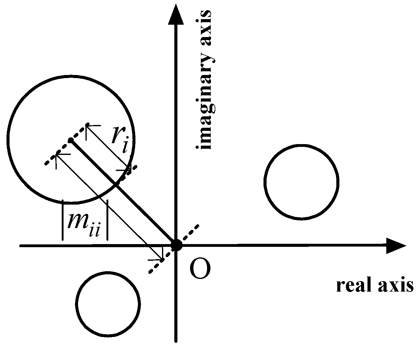
Theorem 1 (Gersgorin theorem [14,17,18]).

Let M be a complex n × n matrix with entries m_ij, then each eigenvalue λ of matrix M locates in the union of n discs.

$${\displaystyle \underset{i=1}{\overset{n}{\cup }}\left|\lambda -m_{ii}\right|\le (r_i={\displaystyle \sum _{\begin{array}{l}i=1\\ j\ne i\end{array}}^n\left|m_{ij}\right|})}$$

(4)

As shown in Figure 1, each disc is called a Gersgorin disc of M. O is the origin. For disc i, m_ii represents the centre; |m_ii| represents the distance from the centre to O; r_i represents the radius of the disc.

According to Equation (4) and Figure 1, l_imin = (|m_ii| − r_i) is the closest distance from disc i to O. And, conclusions can be derived as follows.

(1)

If l_imin ≤ 0, then the origin O is absolutely included in disc i;

(2)

Otherwise, if l_imin > 0, then the origin O can be completely excluded from disc i.

Consequently, if l_imin > 0 can be satisfied for each disc, each disc does not contain the origin O. That is, the origin O can be excluded from the union of all the discs. It means each eigenvalue of M cannot locate at O, and the singular of matrix M can be avoided. For Y, it represents the prevention of harmonic resonance can be realized.

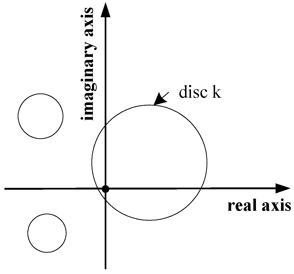
However, for the bus with light load or without loads, the following (5) can be established.

$$y_{kk}\approx -{\displaystyle \sum _{\begin{array}{l}j=1\\ j\ne k\end{array}}^n{y}_{kj}}$$

(5)

where y_kk and y_kj are the diagonal element and off-diagonal element of Y, respectively.

Further, according to the operational laws of vector modules, the following (6) may be established.

$$\left|y_{kk}\right|\le {\displaystyle \sum _{\begin{array}{l}j=1\\ j\ne k\end{array}}^n\left|y_{kj}\right|}$$

(6)

According to the above analysis of (4), Equation (6) means l_kmin ≤ 0. That is, the origin O cannot be excluded from disc k, which is surrounded by the solid line as shown in Figure 2.

Therefore, the prevention of harmonic resonance cannot be guaranteed regardless of the values of the other matrix elements. It means that PFD, which can prevent harmonic resonance, is nonexistent.

The above conclusion is unreasonable in general. Therefore, the basic Gersgorin theorem, namely Formula (4), is not sufficient for evaluating PFD. The three-bus benchmark in Section 5 can intuitively verify the above analysis.

3.2. Study of Matrix Singularity Analysis via the Extended Gersgorin Theorem

To estimate eigenvalues more flexibly, the following Theorem 2, namely the extended Gersgorin theorem, can be further derived via matrix similarity transform (MST).

Theorem 2 [17].

For matrix M = [m_ij] and n positive real numbers (s₁, s₂, …, s_n), then the matrix $\tilde{M}$ = S⁻¹MS, in which S = diag (s₁, s₂, …, s_n), is similar to M. According to the property that similar matrices have the same eigenvalues, each eigenvalue λ of M satisfies the following Formula (7).

$$\left|\lambda -m_{ii}\right|\le \frac{1}{s_i}{\displaystyle \sum _{\begin{array}{l}j=1\\ j\ne i\end{array}}^n{s}_j\left|m_{ij}\right|}(i\in [1,2,\cdots ,n])$$

(7)

For Theorem 2, defining ŕ_i and ĺ_imin as follows.

$$\begin{array}{l}{ŕ}_i=\frac{1}{s_i}{\displaystyle \sum _{\begin{array}{l}j=1\\ j\ne i\end{array}}^n{s}_j\left|m_{ij}\right|}(i\in [1,2,\cdots ,n])\\ {ĺ}_i{}_{\min }=\left|m_{ii}\right|-{ŕ}_i\end{array}$$

(8)

Through comparing Equation (8) with Equation (4), it can be seen that:

(1)

For disc i in Theorem 2, the centre m_ii and |m_ii| remain the same as Theorem 1.

(2)

While the radius ŕ_i is decided by similar transformation matrix (STM) S, namely (s₁, s₂, …, s_n). That is, ŕ_i can be adjusted flexibly with different (s₁, s₂, …, s_n). As a consequence, ĺ_imin, which is the closest distance between disc i and the origin O in Theorem 2, can be adjusted flexibly.

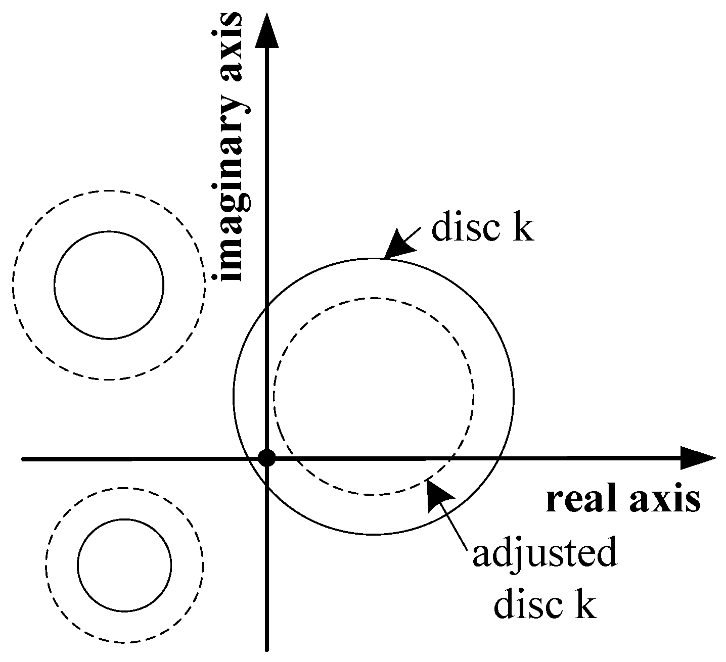
Therefore, as shown in Figure 3, the adjusted disc k may exclude the origin O with appropriate S. Namely, the following Equation (9) may be established with appropriate (s₁, s₂, …, s_n) for Equation (5).

$${ĺ}_i{}_{\min }=(\left|y_{kk}\right|-\frac{1}{s_k}{\displaystyle \sum _{\begin{array}{l}j=1\\ j\ne k\end{array}}^n{s}_j\left|y_{kj}\right|})>0$$

(9)

Further, if ĺ_imin > 0 can be satisfied for each disc with the appropriate (s₁, s₂, …, s_n), each disc does not contain the origin O. For Y, it means the matrix is non-singular and prevention of harmonic resonance is realized.

3.3. Sufficient Condition to Prevent Harmonic Resonance

According to the above analysis via the extended Gersgorin theorem, the sufficient condition to prevent harmonic resonance for Y can be deduced as follows.

$${ĺ}_i{}_{\min }=\left|y_{ii}\right|-{ŕ}_i=\left|y_{ii}\right|-\frac{1}{s_i}{\displaystyle \sum _{\begin{array}{l}j=1\\ j\ne i\end{array}}^n{s}_j\left|y_{ij}\right|}>0 (i\in [1,2,\cdots ,n])$$

(10)

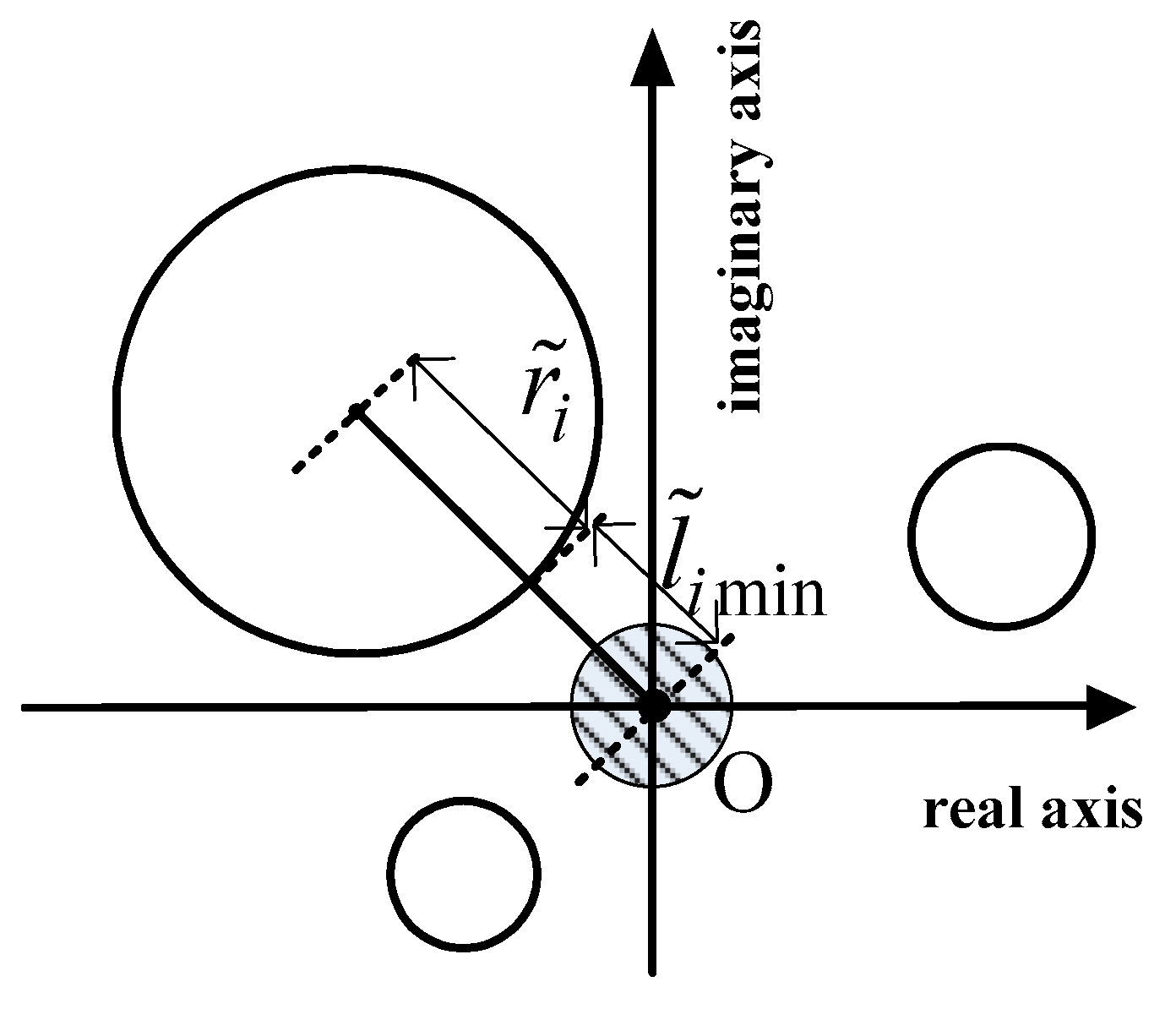
Not just strictly singular, the more common form of Y is nearly singular when harmonic resonance occurs. Therefore, Equation (10) can be modified as the following Equation (11) with a small positive real number ε.

$${ĺ}_i{}_{\min }=\left|y_{ii}\right|-{ŕ}_i=\left|y_{ii}\right|-\frac{1}{s_i}{\displaystyle \sum _{\begin{array}{l}j=1\\ j\ne i\end{array}}^n{s}_j\left|y_{ij}\right|}>\epsilon (i\in [1,2,\cdots ,n])$$

(11)

As shown in Figure 4, Equation (11) means that each estimated disc of Y should evade the shadow disc, whose centre is the origin O and radius is ε, to prevent harmonic resonance.

In this paper, the research objects are equivalent admittance parameters, which are denoted as $\tilde{\mathit{b}}$ = (b₁, b₂, …, b_n), subject to fixed network topology. Also, to realize harmonic resonance prevention, the general sufficient condition is the following Equation (12) for Y with $\tilde{\mathit{b}}$.

$${ĺ}_i{}_{\min }(\tilde{\mathit{b}})=\left|y_{ii}(\tilde{\mathit{b}})\right|-{ŕ}_i =\left|y_{ii}(\tilde{\mathit{b}})\right|-\frac{1}{s_i}{\displaystyle \sum _{\begin{array}{l}j=1\\ j\ne i\end{array}}^n{s}_j\left|y_{ij}\right|}>\epsilon (i\in [1,2,\cdots ,n])$$

(12)

More specifically, the above Equation (12) can be further written as the following form.

$$\{\begin{array}{l}\left|y_{ii}(\tilde{\mathit{b}})\right|-{ŕ}_i>\epsilon (i\in c1)\\ \left|y_{ii}\right|-{ŕ}_i >\epsilon (i\in c2)\\ c1\cup c2=[1,2,3,\cdots ,n]\end{array}$$

(13)

where c1 represents the discs related to $\tilde{\mathit{b}}$; c2 is composed of the discs, which are irrelevant to $\tilde{\mathit{b}}$.

According to Equation (13), once the n positive numbers (s₁, s₂, …, s_n) are determined, ŕ_i can be calculated. And, PFD of $\tilde{\mathit{b}}$ can be obtained from Equation (14) as follows.

$$\left|y_{ii}(\tilde{\mathit{b}})\right|>((\epsilon +{ŕ}_i)=(\epsilon +\frac{1}{s_i}{\displaystyle \sum _{\begin{array}{l}j=1\\ j\ne i\end{array}}^n{s}_j\left|y_{ij}\right|}))(i\in c1)$$

(14)

In the next section, the way to determine (s₁, s₂, …, s_n) is illustrated in detail.

4. Determination of the Optimal STM

From the above Equation (14), it can be seen that PFD of $\tilde{\mathit{b}}$ is directly affected by ŕ_i, which is determined by (s₁, s₂, …, s_n). Moreover, STM of a matrix is non-unique. It means that the obtained PFD can have more than one form. Therefore, the core issue to be discussed is the way to determine the optimal (s₁, s₂, …, s_n) to minimize the conservation of the obtained PFD.

Details are illustrated as follows.

4.1. Conservation Analysis

For illustration purposes, Equation (13) is translated into the following form.

$$\{\begin{array}{l}\left|y_{ii}(\tilde{\mathit{b}})\right|>{ŕ}_i{}_i+\epsilon (i\in c1)\\ s_i(\left|y_{ii}\right|-\epsilon ) >{\displaystyle \sum _{\begin{array}{l}j=1\\ j\ne i\end{array}}^n{s}_j\left|y_{ij}\right|} (i\in c2)\\ s_i>0 (i\in c1\cup c2)\end{array}$$

(15)

From Equation (15), the following conclusions can be deduced.

(1)

For disc $i (i\in c1)$, $\left|y_{ii}(\tilde{\mathit{b}})\right|$ > (ŕ_i + ε) should be met. As shown in Figure 4, the smaller the radius ŕ_i is, the smaller area that $\left|y_{ii}(\tilde{\mathit{b}})\right|$ should avoid in the complex plane. It means that, the larger feasible domain of y_ii($\tilde{\mathit{b}}$), namely, the larger feasible domain of $\tilde{\mathit{b}}$. To sum up, the smaller the radius ŕ_i, the less conservation of the obtained PFD.

(2)

Disc i (i ∈ c2) can be expressed as a linear constraint of (s₁, s₂, …, s_n), in which |y_ii| and |y_ij|are constant.

Therefore, to choose the optimal (s₁, s₂, …, s_n) to guarantee the PFD of $\tilde{\mathit{b}}$ has minimum conservation, the optimization model illustrated in part 2 of this section, can be established.

4.2. The Optimization Model for Choosing the Optimal STM

In this model, the optimization variables are (s₁, s₂, …, s_n).

Specifically, the aim is to minimize the objective function (16).

$$\min {\displaystyle \sum ({ŕ}_i}=\frac{1}{s_i}{\displaystyle \sum _{\begin{array}{l}j=1\\ j\ne i\end{array}}^n{s}_j\left|y_{ij}\right|}) (i\in c1)$$

(16)

In addition, the constraints are as follows.

$$\{\begin{array}{l}{s}_i(\left|y_{ii}\right|-\epsilon ) >{\displaystyle \sum _{\begin{array}{l}j=1\\ j\ne i\end{array}}^n{s}_j\left|y_{ij}\right|} (i\in c2)\\ s_i>0 (i\in c1\cup c2)\end{array}$$

(17)

For the above linear constrained non-linear optimization model, it can be solved easily by sequential quadratic programming (SQP).

By substituting the optimal solution (s_1op, s_2op, …, s_nop) into Equation (14), the optimal PFD of $\tilde{\mathit{b}}$ can be obtained as Equation (18).

$$\left|y_{ii}(\tilde{\mathit{b}})\right|>((\epsilon +{ŕ}_i)=(\epsilon +\frac{1}{s_{iop}}{\displaystyle \sum _{\begin{array}{l}j=1\\ j\ne i\end{array}}^n{s}_{jop}\left|y_{ij}\right|}))(i\in c1)$$

(18)

5. Case Studies

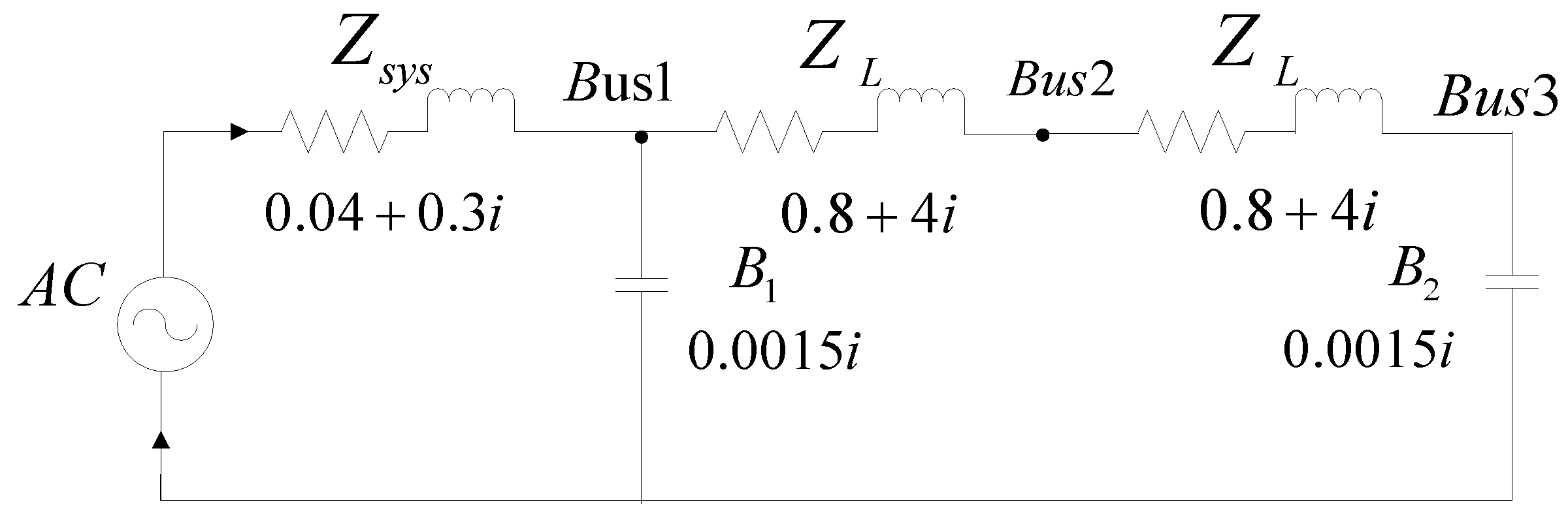
Availability and superiorities of the method in this paper are verified through four different scale systems. Concretely, a 3-bus benchmark [5] as shown in Figure 5, and a modified 9-bus benchmark, a modified 27-bus benchmark and a modified 81-bus benchmark, which are based on the proposed universal benchmark illustrated in part 2 of this section.

The 3-bus benchmark is used to demonstrate the analysis and computation processes of the proposed method clearly, and the other three benchmarks are used to analyze the effects of system scale and variable parameter number on the computation efficiency and conservation of the proposed method.

5.1. PFD of the 3-Bus Benchmark

The values of the parameters in Figure 5 are the impedances and admittances under the fundamental frequency f₁, respectively. f = 9f₁ is selected as the frequency to be analyzed. Also, a continuous adjustable component whose equivalent admittance parameter under f is b_f ∈ [−0.1, 0.1], is assumed to be installed on bus 3.

To prevent harmonic resonance at frequency f, PFD of b_f is to be sought. As the basis, the harmonic network admittance matrix Y_f is obtained as in Equation (19) below.

$$Y_f=\left[\begin{array}{ccc}0.0061-0.3846i& -0.0006+0.0278i& 0\\ -0.0006+0.0278i& 0.0012-0.0555i& -0.0006+0.0278i\\ 0& -0.0006+0.0278i& 0.0006+(b_f-0.0143)i\end{array}\right]$$

(19)

where i is $\sqrt{-1}$.

5.1.1. Analysis Based on Pointwise Precise Eigenvalue Computation (Method 1)

As the first step, the method based on pointwise precise eigenvalue computation, namely Method 1, is carried out, to sweep the whole variation range of b_f.

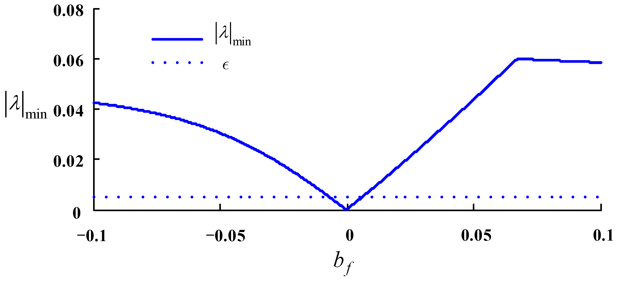
Specifically, according to the values in Figure 5 and Equation (19), the pointwise step is set as 0.0001. Using Method 1, the change of the minimum module of eigenvalues, entitled as |λ|_min, with b_f can be obtained as the solid line shown in Figure 6. Time consumption of the above pointwise process is 0.0239 s. All the results of this paper are obtained by a PC, whose CPU is [email protected] GHZ and RAM is 8 G, and the software environment is Windows 10 Professional and MATLAB R2010b. All the data of time consumption in Section 5 is the average for more than 10 times running of the methods.

From Figure 6, it can be seen that |λ|_min is about between 0.02 and 0.05 for most regions of b_f. And, when |λ|_min is under 0.005, it is very close to zero, which indicates the occurrence of harmonic resonance. Therefore, for Equation (19), ε is set as 0.005, and the PFD can be obtained as b_f ∈ [−0.1, −0.0066]∪[0.0060, 0.1], by the principle that |λ|_min should be greater than ε (as the dotted line in Figure 6).

Further, the methods using eigenvalue estimation are carried out.

5.1.2. Analysis Based on Basic Gersgorin Theorem

On one hand, the basic Gersgorin theorem is used. From Equation (19), the following Equation (20) can be obtained.

$$Y_f(2,2)=-(Y_f(2,1)+Y_f(2,3)) =1/(0.8+4\times 9i)+1/(0.8+4\times 9i)$$

(20)

Therefore,

$$\left|Y_f(2,2)\right|=\left|Y_f(2,1)\right|+\left|Y_f(2,3)\right|$$

(21)

According to the analysis of the basic Gersgorin theorem in Section 3.1, Equation (21) means l_2min ≤ 0. Therefore, the origin O cannot be excluded from disc 2. It means that the prevention of harmonic resonance cannot be guaranteed regardless of the b_f value. That is, PFD is nonexistent.

Compared with b_f ∈ [−0.1, −0.0066]∪[0.0060, 0.1], which is obtained by Method 1, the above conclusion is obviously unreasonable. Therefore, it verifies that the basic Gersgorin theorem is not sufficient for analyzing PFD.

5.1.3. Analysis Based on the extended Gersgorin Theorem (Method 2)

On the other hand, the proposed method based on the extended Gersgorin theorem, namely Method 2, is carried out. Concrete implement processes are as follows.

According to Equation (11) in Section 3, prevention of harmonic resonance can be realized if the following Equation (22) is satisfied.

$$\{\begin{array}{l}0.3846-\epsilon >\frac{s_2}{s_1}0.0278\\ 0.0555-\epsilon >\frac{s_1}{s_2}0.0278+\frac{s_3}{s_2}0.0278\\ \sqrt{{0.0006}^2+{(b_f-0.0143)}^2}-\epsilon >\frac{s_2}{s_3}0.0278\end{array}$$

(22)

As the dotted line in Figure 6, ε equals to 0.005 to keep Y_f away from singular. Hence, the optimization model (23) can be established in accordance with Equations (16) and (17) in Section 4.

$$\begin{array}{l}\min (\frac{s_2}{s_1}0.0278)\\ \{\begin{array}{l}{s}_1(0.3846-0.005)>s_{2}0.0278\\ s_2(0.0555-0.005)>s_{1}0.0278+s_{3}0.0278\\ s_1>0,s_2>0,s_3>0\end{array}\end{array}$$

(23)

For the above linear constrained non-linear optimization model, SQP is used to solve it. The optimal result is s_1op = 0.0690, s_2op = 0.9417, s_3op = 1.6416. Time consumption of the above optimization process is 0.0047 s. Eventually, PFD of b_f can be obtained through the following (24) in accordance with Equation (18).

$$\{\begin{array}{l}\sqrt{{0.0006}^2+{(b_f-0.0143)}^2}>\frac{0.9417}{1.6416}\times 0.0278+0.005\\ -0.1\le b_f\le 0.1\end{array}$$

(24)

In addition, the result is derived as b_f ∈ [−0.1, −0.0066)∪(0.0352, 0.1].

More important, PFD of b_f on the condition that s₂/s₃ is greater than the above minimum value of 0.5736 is calculated for comparison. Set s₂/s₃ as 0.7, b_f ∈ [−0.1, −0.0102)∪(0.0388, 0.1] can be obtained. It can be seen that [−0.1, −0.0102) and (0.0388, 0.1] are the subsets of [−0.1, −0.0066) and (0.0352, 0.1], respectively. It shows that the conservation of PFD can be reduced via optimization of STM.

5.1.4. Comparisons of the Methods

From the above results, the proposed Method 2 shows good applicability. For illustration purposes, detailed results of the two methods are listed in

Table 1. Results of PFD via the two methods.

Method	Time Consumption, s	PFD of bf
Method 1	0.0239	[−0.1, −0.0066]∪[0.0060, 0.1]
Method 2	0.0047	[−0.1, −0.0066)∪(0.0352, 0.1]

below.

By comparing the results in Table 1, conclusions are deduced as follows.

(1)

In the view of time consumption, Method 2 is much less than Method 1. Concretely, time consumptions of Method 1 and Method 2 are 0.0239 s and 0.0047 s, respectively. The rapidity of the proposed method is realized by avoiding time-consuming pointwise precise eigenvalue computations via estimation of eigenvalues.

(2)

In the view of the range of obtained PFD, the result of Method 2 is the subset of the result of Method 1. Though the PFD of the proposed method is conservative, it covers most of the region of the PFD of Method 1. Concretely, [−0.1, −0.0066) and [−0.1, −0.0066] are almost the same, while (0.0352, 0.1] is the subset of [0.0060, 0.1]. Conservation of the proposed method is inevitable, as the derived condition is not the necessary and sufficient condition.

5.2. Effects of System Scale on Time Consumption and Conservation

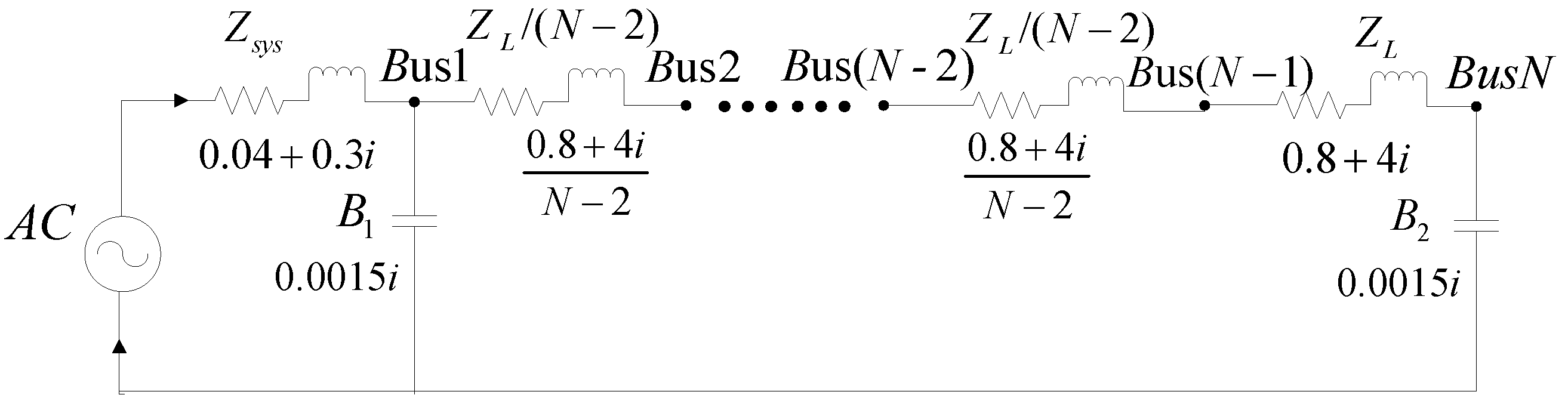
From the existing analyses in this paper, it can be seen that the self-admittance of the bus with b_f affects the result of PFD. To analyze the effects of bus number on conservatism and time consumption of the proposed method, the universal benchmark as shown in Figure 7 is designed according to control variable method based on the 3-bus benchmark of Figure 5. For the universal benchmark, Y_f(N,N) is constant. The same continuous adjustable component, whose equivalent admittance parameter under f is b_f ∈ [−0.1, 0.1], is assumed to be installed on bus N.

Also, for convenience of consistent evaluation of the range of PFD, ε equals the value of |λ|_min under b_f = −0.0066 for the universal N-bus benchmark.

For N equals to 9, 27, 81, Method 1 and Method 2 are carried out, respectively. Pointwise steps are all set as 0.0001. Detailed results are listed in

Table 2. Results of Method 1 for different scale benchmarks.

N	ε	Time Consumption, s	PFD of bf
9	0.00314	0.0614	[−0.1, −0.0066]∪[0.0051, 0.1]
27	0.00134	0.4437	[−0.1, −0.0066]∪[0.0038, 0.1]
81	0.000484	9.5168	[−0.1, −0.0066]∪[0.0032, 0.1]

and

Table 3. Results of Method 2 for different scale benchmarks.

N	ε	Time Consumption, s	PFD of bf
9	0.00314	0.0056	[−0.1, −0.0066)∪(0.0351, 0.1]
27	0.00134	0.0095	[−0.1, −0.0066)∪(0.0351, 0.1]
81	0.000484	0.0288	[−0.1, −0.0066)∪(0.0351, 0.1]

below.

In the view of time consumption, the following conclusions are deduced from Table 1, Table 2 and Table 3.

(1)

When bus number increases, time consumptions of Method 1 and Method 2 are both increased.

(2)

Compared with Method 1, time consumption of the proposed Method 2 increases much more slowly.

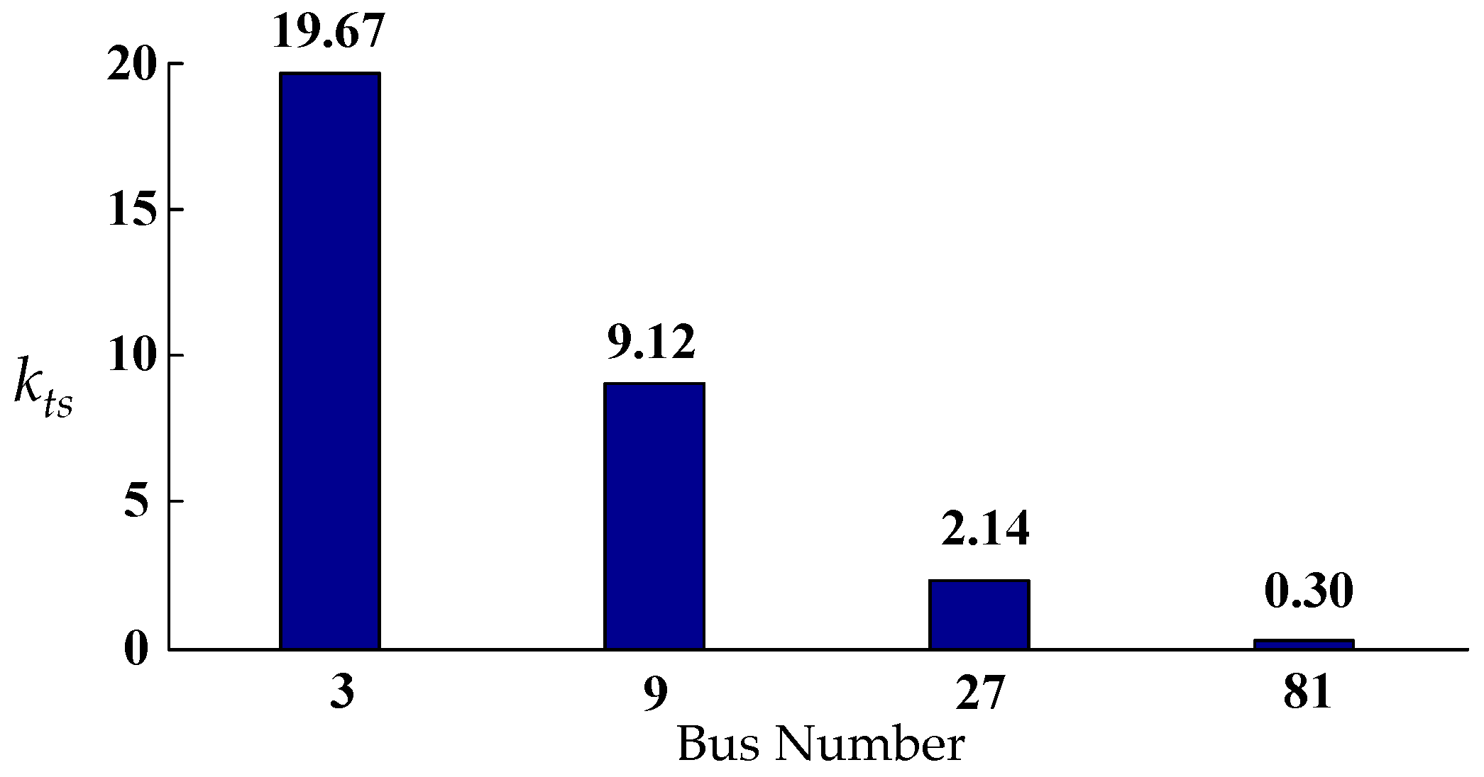
For quantitative comparison, an index of time consumption ratio is defined as k_ts.

$$k_{ts}=\frac{t_{m2}}{t_{m1}}\times 100\%$$

(25)

where t_m1 and t_m2 are the time consumptions of Method 1 and Method 2, respectively. From Table 1, Table 2 and Table 3, the change of k_ts corresponding to the change of bus number is shown in Figure 8.

As shown in Figure 8, k_ts shows a trend of quick decrease with the enlargement of system scale. When the bus numbers are 3, 9, 27 and 81, k_ts are 19.67%, 9.12%, 2.14% and 0.30%, respectively.

In the view of the range of PFD, the following conclusion is deduced from Table 1, Table 2 and Table 3.

When bus number increases, the conservation of the proposed method increases very slightly.

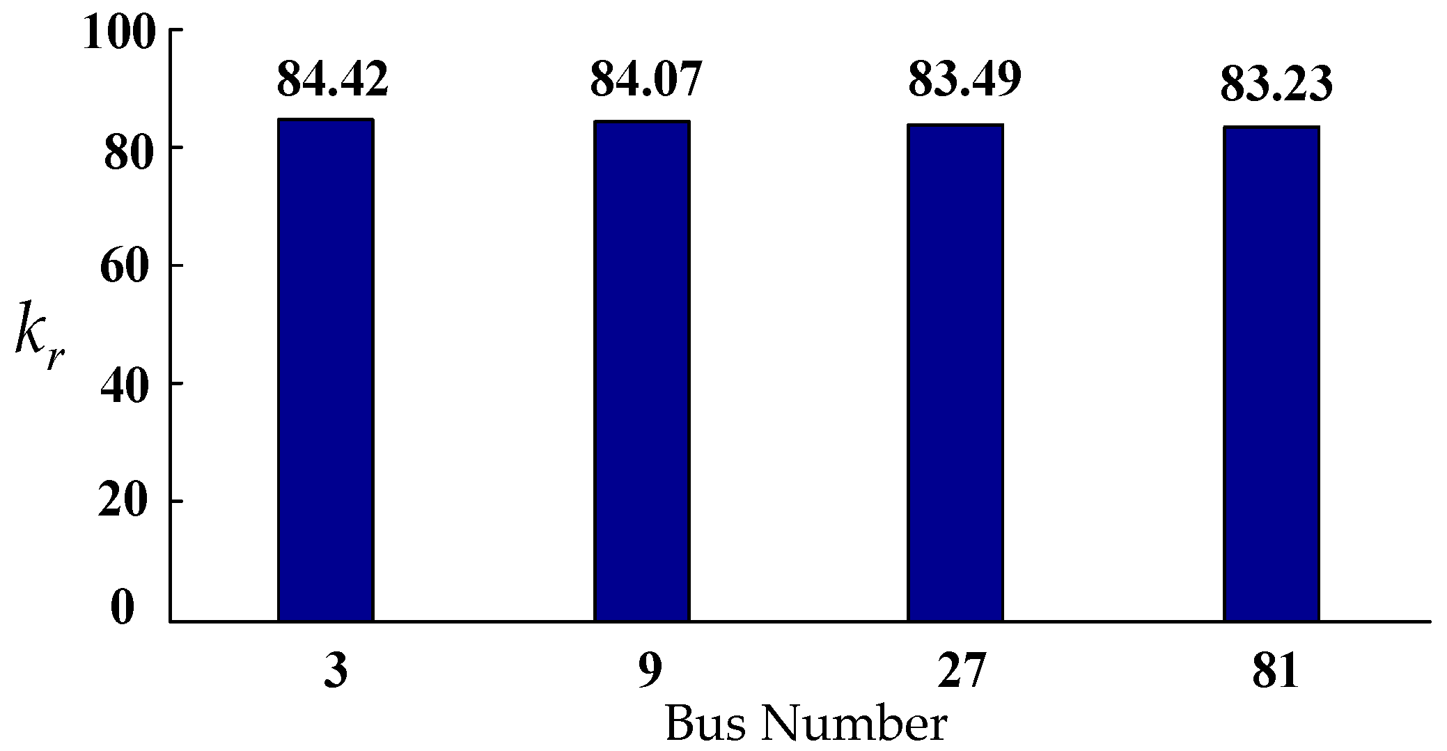
Similarly, the following index of covering-ratio k_r is defined for quantitative comparison.

$$k_r=\frac{r_{m2}}{r_{m1}}\times 100\%$$

(26)

where r_m1 and r_m2 are the widths of obtained PFD via Method 1 and Method 2, respectively. From Table 1, Table 2 and Table 3, the change of k_r corresponding to the change of bus number is shown in Figure 9.

As shown in Figure 9, k_r shows a trend of very light decrease with the enlargement of system scale. That is, the conservation of the proposed method increased very slightly. When the bus numbers are 3, 9, 27 and 81, k_r are 84.42%, 84.07%, 83.49% and 83.23%, respectively.

To sum up, it shows that the advantage of Method 2 in time consumption is rapidly amplified with the enlargement of system scale, while the conservation increases very slightly.

5.3. Effect of Variable Parameter Number on Time Consumption

To analyze the effect of the number of variable parameters, the following tests are implemented. Set N as 11 for the universal benchmark, Method 1 and Method 2 are employed for three scenarios with only one variable parameter, two variable parameters and three variable parameters, respectively. All the variable parameters are continuous adjustable equivalent admittances with the same variation ranges of [−0.1, 0.1] and pointwise steps of 0.0001. Corresponding results of time consumptions are shown in

Table 4. Time consumptions with the enlargement of variable parameter number.

Variable Parameter Number	Time Consumption, s
	Method 1	Method 2
1	0.0726	0.0061
2	1.3418 × 102	0.0085
3	2.4596 × 105	0.0115

below.

By comparing the results in Table 4, conclusions are deduced as follows.

(1)

When variable parameter number increases, time consumptions of Method 1 and Method 2 are both increased.

(2)

Compared with Method 1, time consumption of Method 2 increases much more slowly. Concretely, for the above three scenarios, time consumptions of Method 1 are 0.0726 s, 1.3418 × 10² s and 2.4596 × 10⁵ s, which shows a trend of explosive increase. In contrast, time consumptions of the proposed Method 2 are merely 0.0061 s, 0.0085 s and 0.0115 s.

To sum up, it shows that the advantage of Method 2 in time consumption is more significant with the enlargement of the variable parameter number.

5.4. Improvement of Offline Analysis Efficiency of PFD Using the Proposed Method

According to the above comparative analyses, the proposed method shows remarkable superiorities in online evaluation of PFD. In addition, it can be used to improve the efficiency of offline evaluation of PFD as well.

Method 3, in which the proposed method is applied to give preliminary evaluation of PFD, and Method 1 is employed to sweep the rest parameter space to amend the domain, is proposed. Using Method 3 to analyze the 3-bus benchmark, results listed in

Table 5. Results of Method 3 for the 3-bus benchmark.

Method	Time Consumption, s	PFD of bf
Method 3	0.0093	[−0.1, −0.0066]∪[0.0060, 0.1]

can be obtained.

From Table 1 and Table 5, it can be found that:

(1)

In the view of time consumption, Method 3 is merely 38.91% of Method 1.

(2)

In the view of the range of PFD, Method 3 is the same as Method 1.

For the other three benchmarks, similar results can be obtained as well. Concretely, time consumption results are listed in

Table 6. Time consumptions of Method 1 and Method 3 for the other three benchmarks.

N	Time Consumption, s
	Method 1	Method 3
9	0.0614	0.0182
27	0.4437	0.1003
81	9.5168	2.0841

.

From Table 1, Table 5 and Table 6, it can be found that time consumptions of Method 3 are 38.91%, 29.64%, 22.61% and 21.90% of Method 1 for the four benchmarks, respectively.

Therefore, via preliminary evaluation using the proposed method, the offline analysis efficiency of PFD can be improved.

6. Conclusions

In this paper, a novel evaluation method of PFD is proposed. Firstly, the sufficient condition to prevent harmonic resonance is derived in the view of the singularity of harmonic network admittance matrix, via the extended Gersgorin theorem. Further, to reduce the conservation of the obtained PFD, a strategy is proposed to search the optimal STM, according to the non-uniqueness of STM. Eventually, availability and advantages of the method are demonstrated through different scale benchmarks.

(1)

Via introducing MST, the inapplicability of the basic Gersgorin theorem for evaluating PFD is overcome. Through the proposed strategy to determine the optimal STM, reduction of the conservation of the obtained PFD is realized.

(2)

It is suitable to implement online assessment of PFD in power grid. Compared with the pointwise precise eigenvalue computation-based method, it shows much better performance in analysis efficiency. Moreover, the larger the system scale or the greater the number of variable parameters, the more significant the advantage in computation efficiency.

(3)

Besides, it can be used as preliminary assessment to improve offline analysis efficiency of PFD in power grid as well.

As the proposed method is put forward based on the derived sufficient condition, conservation is inevitable. More researches will be done to seek the way to further reduce the conservation in future work. Furthermore, theoretical method to determine ε will be sought as well.