Variable Speed Control of Wind Turbines Based on the Quasi-Continuous High-Order Sliding Mode Method

Abstract

The characteristics of wind turbine systems such as nonlinearity, uncertainty and strong coupling, as well as external interference, present great challenges in wind turbine controller design. In this paper, a quasi-continuous high-order sliding mode method is used to design controllers due to its strong robustness to external disturbances, unmodeled dynamics and parameter uncertainties. It can also effectively suppress the chattering toward which the traditional sliding mode control method is ineffective. In this study, the strategy of designing speed controllers based on the quasi-continuous high order sliding mode method is proposed to ensure the wind turbine works well in different wind modes. First, the plant model of the variable speed control system is built as a linearized model; and then a second order speed controller is designed for the model and its stability is proved. Finally, the designed controller is applied to wind turbine pitch control. Based on the simulation results from a simulation of 1200 s which contains almost all wind speed modes, it is shown that the pitch angle can be rapidly adjusted according to wind speed change by the designed controller. Hence, the output power is maintained at the rated value corresponding to the wind speed. In addition, the robustness of the system is verified. Meanwhile, the chattering is found to be effectively suppressed.

1. Introduction

The technical development of wind power is partially represented by the development of wind turbine control technology. Various control methods such as robust control, adaptive control, back stepping control, sliding mode control, model predictive control and so on have been proposed and studied [1,2,3,4,5]. Among these methods, sliding mode control has been proven to be robust with respect to system parameter variations and external disturbances, and it can quickly converge to the control target.

In practical application, proportional integral derivative (proportional integral differential, PID) controller or proportional integral (PI) controllers are widely applied. In these the controller parameters are obtained based on experience and/or on-site testing as no theoretical system is used for the calculation, thereby lacking a proved stability and causing security risk. The ultimate goal to control wind turbine is to provide safe and stable operation in the whole process, to reach the regional specific control objectives, and to provide safe and reliable power production. Therefore, the study of advanced, intelligent, stable, and secure control technology has become so important [6] that many scholars worldwide have made efforts to develop new control techniques, especially control techniques applied to pitch control.

In the early studies, the classical P/PI/PID pitch angle controllers based on linearized models have been implemented [7,8,9,10]. In those studies, however, wind turbine control design is based on experimental models [11]. A simple control scheme for variable speed wind turbines is given in [12], and a comparison of nonlinear and linear model-based design of variable speed wind turbines is presented in [13].

In [14,15], the use of integral sliding-mode control method combined with the improved Newton-Raphson wind speed estimator is proposed to design the controller to control the generator torque so as to adjust the rotor speed for achieving the maximum energy conversion of the wind turbine. The control stability is investigated by the Lyapunov function analysis. In order to maximize the efficiency of energy conversion and reduce mechanical stress of main shaft, in [16], an adaptive second order sliding mode control strategy with variable gain is formulated through improvement of the super-twisting algorithm. This control strategy is able to deal with the randomness of wind speed, the non-linearity of wind turbine systems, uncertainty of the model and the influence of external disturbances.

In [17], the traditional sliding mode control strategy is used to control the power of a variable speed wind turbine. The ideal feedback control tracking under uncertain and disturbing conditions is realized, which ensures the stability of the two operating regions and the strong robustness of the control system. Reference [18] proposed a high-order sliding mode control method for power control. The algorithm is simple and reliable, and the generator torque chattering is small, thereby greatly improving the efficiency of wind energy conversion. Reference [19] proposed a continuous high-order sliding mode control method for nonlinear control of the variable speed wind turbine system, which is combined with the maximum power point tracking (MPPT) algorithm to ensure the optimal power output tracking, better system dynamic performance and strong robustness.

The randomness and uncertainty of wind speed, the non-linearity of wind turbine systems and the presence of external disturbances make it difficult to establish accurate mathematical models for modelling the wind turbine subsystems. Under this situation and owing to the strong robustness of the control method to external disturbances, unmodeled dynamics and parameter uncertainties; the sliding mode control has been widely utilized. In addition, the control method has advantages of simple control law and fast dynamic response. As the traditional sliding mode control is prone to severe chattering, it is difficult to maintain the system stability. As a result, it is only applicable to the relative order 1 system. In order to overcome the issue, this paper proposes a high-order sliding mode control method for pitch control and speed control of the wind turbines. This method can effectively weaken the chattering phenomenon and realize any order control while achieving the traditional control target.

The remainder of this paper is organized as follows: Section 2 introduces the sliding mode control method, Section 3 describes the control models, Section 4 presents the design of the controllers and its stability, and Section 5 discusses the simulation results. Finally, it is concluded as shown in Section 6.

2. Introduction to High-Order Sliding Mode Control

2.1. Conventional Sliding Mode Control

Sliding mode control is defined and described in [20]. It is a nonlinear control method that alters the dynamics of a nonlinear system by application of a discontinuous control signal that forces the system to “slide” along a cross-section of the system’s normal behavior. However, the conventional sliding mode control has the following shortcomings.

2.1.1. Chattering ${\omega }_{ls}$

The sliding mode motion causes the state of the system to continue to move up and down at a low amplitude and high frequency along a predetermined trajectory, but the actual sliding mode does not occur strictly on the sliding surface due to the inertia and hysteresis of the switching device, thereby triggering a high-frequency switching of the control, resulting in chattering [21]. This kind of chattering phenomenon will not only reduce the accuracy of system control and increase the energy loss, but also easily stimulate the high frequency unmodeled dynamics resulting in damage of the system stability and even damage of the controlled device.

2.1.2. Limited Relative Order

The conventional sliding mode control can only be applied to systems with relative order 1, i.e., the control variable must appear explicitly on the sliding surface.

2.1.3. Low Control Accuracy

For discrete conventional sliding mode control systems, the system sliding error is proportional to the sampling time, that is, the accuracy of the system state remaining in the sliding mode is the first order infinitesimal of the sampling time.

2.2. High-Order Sliding Model Control

In 2003, Levant [22] proposed a sliding mode control method with finite-time convergence for system with arbitrary relative order and a quasi-continuous high-order sliding mode control (QCHOSM) method, in which the proposed high-order sliding mode controller is the common convergent controller in the finite time. It is used to control any uncertain system with arbitrary relative order with the advantages of short convergence time and strong robustness.

For a single input and single output system:

$$\dot{x}(t)=f(t,x)+g(t,x)u$$

(1)

where x(t) is system state vector and u is input of the control, with relative order of r of sliding surface s(t, x) = 0, the control target is to make the system state move to s(t, x) = 0 within a limited time in the rth order sliding mode. This means that:

$$s=\dot{s}=\ddot{s}=\cdots =s^{(r-1)}=0.$$

(2)

If r is known in the system, the following is obtained:

$$s^{(r)}=h(t,x)+g(t,x)u$$

(3)

where $h(t,x)=s^{(r)}{|}_{u=0}$, $g(t,x)=\frac{\partial }{\partial u}{s}^{(r)}$ ≠ 0. And there exist K_m, K_M, and C > 0 for [14]:

$$0\le K_m\le \frac{\partial }{\partial u}{s}^{\left(r\right)}\le K_M$$

(4)

where $\left|s^{\left(r\right)}{|}_{u=0}\right|\le 0$.

When Equation (1) is true, any continuous input u = $U\left(s, \dot{s, }\cdots s^{\left(r-1\right)}\right)$ satisfies $U(0,0,\cdots ,0)=-h(t,x)/g(t,x)$ for s ≡ 0. Because of uncertain factors existing in the system, u = $U\left(s, \dot{s, }\cdots s^{\left(r-1\right)}\right)$ in Equation (1) is not continuous at least, then it can be converged to $s^{\left(r\right)}$ [19,20]. From Equations (3) and (4), the following solution exits in Filippov:

$$s^{\left(r\right)}\in \left[-C,C\right]+\left[K_m,K_M\right]u.$$

(5)

In summary, r-order sliding mode control is defined as design the sliding surface s, and construct the discontinuous controller u = $U(s, \dot{s, }\cdots s^{\left(r-1\right)})$ to make the system trajectory finally stabilize onto $s^{\left(r\right)}$.

For any order sliding mode control with $q$ being a positive constant and $q\ge r$, Levant [22] proposed the following control equations:

$$\{\begin{array}{l}{N}_{1,r}={\left|s\right|}^{(r-1)/r}\\ N_{i,r}={\left({\left|s\right|}^{q/r}+{\left|\dot{s}\right|}^{q/(r-1)}+\cdots +{\left|s^{(i-1)}\right|}^{q/(r-i+1)}\right)}^{(r-i)/q}\\ N_{r-1,r}={\left({\left|s\right|}^{q/r}+{\left|\dot{s}\right|}^{q/(r-1)}+\cdots +{\left|s^{(r-2)}\right|}^{q/2}\right)}^{1/q},i=1,2,\cdots ,r\\ {\varphi }_{0,r}=s\\ {\varphi }_{1,r}=\dot{s}+{\beta }_1{N}_{1,r}\mathrm{sgn}(s)\\ {\varphi }_{i,r}=s^{(i)}+{\beta }_i{N}_{i,\text{}r}\mathrm{sgn}({\varphi }_{i-1,r}),i=1,2,\cdots ,r-1\end{array}$$

(6)

where β₁, β₂, …, β_r−1 are positive and obtained by simulation tests.

Theorem 1. 

Assume the system expressed by Equation (1) has the relative order r on s and satisfies Equation (5), and its trajectory can be unlimitedly extended in time for any order Lebesgue measurable and bounded control, the control law:

$$u=-k\cdot \mathrm{sgn}\left({\varphi }_{r-1,r}(s,\dot{s},\cdots s^{(r-1)})\right)$$

(7)

is able to ensure that the r-order sliding mode converged in finite time exists, and the convergence time is the locally bounded function of the initial condition for appropriately determined positive values of ${\beta }_1$, ${\beta }_2$, …, ${\beta }_{r-1}$ and k.

For the system with relative order r which is less than 4, the controller expression was presented in [23] as follows:

$$\{\begin{array}{ll}(1)& u=-k\cdot \mathrm{sgn}s\\ (2)& u=-k(\dot{s}+{\left|s\right|}^{1/2}\mathrm{sgn}s)/(\left|\dot{s}\right|+{\left|s\right|}^{1/2})\\ (3)& u=-k\frac{\ddot{s}+2{(\left|\dot{s}\right|+{\left|s\right|}^{2/3})}^{-1/2}(\dot{s}+{\left|s\right|}^{2/3}\mathrm{sgn}s)}{\left|\ddot{s}\right|+2{(\left|\dot{s}\right|+{\left|s\right|}^{2/3})}^{1/2}}\\ (4)& {\phi }_{3,4}=\ddot{s}+3\left[\ddot{s}+{(\left|\dot{s}\right|+0.5{\left|s\right|}^{3/4})}^{-1/3}(\dot{s}+0.5{\left|s\right|}^{3/4}\mathrm{sgn}s)\right]{\left[\left|\ddot{s}\right|+{(\left|\dot{s}\right|+0.5{\left|s\right|}^{3/4})}^{2/3}\right]}^{-1/2}\\ & N_{3,4}=\ddot{s}+3{\left[\left|\ddot{s}\right|+{(\left|\dot{s}\right|+0.5{\left|s\right|}^{3/4})}^{2/3}\right]}^{1/2}\\ & u=-k{\phi }_{3,4}/N_{3,4}\end{array}$$

(8)

which is derived from Equations (6) and (7).

Through high-order sliding mode, the control algorithm can be constructed on any order derivative of the sliding mode. However, the calculation of the control algorithm requires the information of the derivative of the previous order system variables. For example, the controller (8) needs the sliding surface and its real-calculated value or direct measure of its real time derivatives with respect to time. However, the higher order derivatives of these state variables do not necessarily have physical meaning and the sensitivity to noise makes these higher order derivatives not be directly measured by the sensor [24]. In order to solve these problems, Levant designed a finite time-convergent robust differentiator with high precision by considering the effect of noise based on the high-order sliding mode theory.

In practical application of high-order sliding mode, the value of the sliding surface and its first derivative can be estimated by Levant Robust Differentiator:

$$u=-k\cdot \mathrm{sgn}\left({\varphi }_{r-1,r}(z_0,z_1,\cdots z_{r-1})\right)$$

(9)

where $z_0, z_1, \cdots , z_{r-1}$ are sliding surface and derivatives, respectively. Levant sliding differentiator is constituted by a first order differentiator in real time as [25]:

$$\{\begin{array}{l}{\dot{z}}_0={\upsilon }_0\\ {\upsilon }_0=-{\lambda }_r{L}^{1/r}{\left|z_0-s\right|}^{(r-1)/r}\mathrm{sgn}(z_0-s)+z_1\\ {\dot{z}}_k={\upsilon }_k\\ {\upsilon }_k=-{\lambda }_{r-k}{L}^{1/(r-k)}{\left|z_k-{\upsilon }_{k-1}\right|}^{(r-k-1)/(r-k)}\mathrm{sgn}(z_k-{\upsilon }_{k-1})+z_{k+1},k=1,\cdots ,r-2\\ {\dot{z}}_{r-1}=-{\lambda }_{1}L\mathrm{sgn}(z_{r-1}-{\upsilon }_{r-2})\end{array}$$

(10)

The values of k in Equations (7) and (8), and value of L in Equation (10) are obtained by simulation. L in Equation (10) should be large enough to ensure that the system has good performance in the presence of measurement error. Usually in the simulation the following parameter values are used: L = 400, λ₁ = 1.1, λ₂ = 1.5, λ₃ = 2.0, λ₄ = 3.0, λ₅ = 5.0 and λ₆ = 8.0 [25].

3. Models of Variable Speed Controller

From the knowledge of aerodynamics, the operation of the variable speed and variable pitch wind turbine can be divided into four regions [26] according to the cut-in wind speed, rated wind speed and cut-out wind speed during the whole wind speed changing process, as shown in Figure 1.

In region I, wind speed does not reach the cut-in wind speed, the generator is turned on but the turbine cannot generate sufficient power due to the large inertia of the rotating parts. In this region, the system is in feathering state, pitch angle is β = 90° and the starting torque is relatively large.

In region II, wind speed is higher than the cut-in wind speed and lower than the rated wind speed. The pitch angle is constant in all of this region, and the generator torque is used as the control input to adjust the turbine rotor speed to capture the wind power as much as possible.

In region III, wind speed is between the rated wind speed and cut-out wind speed. In order to ensure that the electrical and mechanical loads in safe state, the pitch actuator is required to adjust the pitch angle and reduce the wind turbine power conversion efficiency to stabilize the turbine output power in the vicinity of the rated power [27].

In region IV, wind speed is higher than the cut-out wind speed. Cut-out speed is the maximum speed of the wind for power production. When wind speed is higher than the cut-out speed, the wind turbine is shut down without any power production; otherwise, it will lead to damage to the wind turbine.

In this paper, the controllers are designed for pitch control with wind speed in the regions from II to IV.

3.1. Wind Turbine Model

From aerodynamics, the mechanical power captured by the wind turbine from wind energy is known as [28]:

$$P_a=\frac{1}{2}\rho \pi R^2{C}_p(\lambda ,\beta )v^3$$

(11)

where C_p(λ, β) represents the wind turbine power conversion efficiency, used to characterize the efficiency of the wind turbine converting wind energy to mechanical energy, which is associated with tip speed ratio λ and pitch angle β, and is defined as [2]:

$$C_p(\lambda ,\beta )=c_1(\frac{c_2}{{\lambda }_i}-c_3\beta -c_4)e^{-\frac{c_5}{{\lambda }_i}}+c_6\lambda$$

(12)

with:

$$\frac{1}{{\lambda }_i}=\frac{1}{\lambda +0.08\beta }-\frac{0.035}{{\beta }^3+1}$$

(13)

and $c_1$ = 0.5176, $c_2$ = 116, $c_3$ = 0.40, $c_4$ = 5.0, $c_5$ = 21.0, $c_6$ = 0.0068 [2]. The values of coefficients $c_1$ to $c_6$ depend on the specific environment, the turbine blade shape profile and its aerodynamic performance. λ is calculated as:

$$\lambda =R\frac{{\omega }_r}{v}$$

(14)

where ${\omega }_r$ is turbine rotor speed (rad/s). For different pitch angle values, there is an optimal tip speed ratio λ_opt, making it work continuously along with the change of wind speed on the best working point, then the wind turbine conversion efficiency is the highest.

The mechanical power expressed in terms of aerodynamic torque is shown in Equation (15):

$$P_a={\omega }_r{T}_a$$

(15)

where T_a is aerodynamic torque (N·m), defined as:

$$T_a=\frac{1}{2}\pi \rho R^3\frac{C_p(\lambda ,\beta )}{\lambda }{v}^2.$$

(16)

3.2. Generator Model

In addition to considering the reliability and operating life of the generator, it is also necessary to consider whether it can adapt to the different changes of wind conditions and provide stable electrical energy.

In pitch control, it is to adjust the pitch angle with response to the required generator output torque and rotational speed in order to maintain a constant state. For the commonly used asynchronous generator, the generator torque is expressed as [29]:

$$Te=\frac{g{m}_1{U}_1^2{r}_2\prime }{({\omega }_g-{\omega }_1)[{(r_1-\frac{C_1}{{\omega }_g-{\omega }_1})}^2+{(x_1+C_1{x}_2\prime )}^2]},$$

(17)

$${\omega }_g=n_g{\omega }_r.$$

(18)

When wind speed is above the rated wind speed, it is necessary to start the propeller actuator to restrict the wind energy captured by considering the load bearing capacity of the wind turbine and the limitation of the performance index of each component. The pitch control system adjusts the pitch angle which is determined by the wind speed. The blade pitch is driven by the servo motor. Its mathematical model is given below:

$${\tau }_{\beta }\dot{\beta }={\beta }^{\ast }-\beta$$

(19)

where ${\beta }^{*}$ is the reference value of the pitch angle (°); β is the actual output pitch angle (°), and ${\tau }_{\beta }$ is a time constant. This is actually a first-order delay link because the drive system itself has some computing delay, conditional delay, etc. so that the propeller actuator cannot do real-time response [27]. The rotor actuator model can also be expressed as:

$$G_p(s)=\frac{\beta (s)}{{\beta }^{\ast }(s)}=\frac{1}{{\tau }_{\beta }s+1}.$$

(20)

In summary, the control strategy for the variable speed stage is obtained in the following way, i.e., when the wind speed is lower than the rated wind speed, the generator torque is controlled so that the turbine rotor speed can be adjusted quickly to find the best power output point and maximize the wind energy conversion efficiency. The wind turbine speed control scheme is shown in Figure 2, where P_a represents the power captured by the wind turbine from the wind.

3.3. Nonlinear-Controlled Object Model

In the condition of a control system involving the model uncertainty and external disturbance, and the wind speed is higher than the rated wind speed; variable pitch control is utilized to which a newly proposed quasi-continuous high order sliding mode control method is applied. The control system design needs to take into account the following aspects: pitch control strategy, the controlled object model, accurate feedback linearization, controller design, stability verification and simulation analysis.

The controlled object model of wind turbine is expressed by Equation (21) [18]:

$$\{\begin{array}{l}{J}_r{\dot{\omega }}_r=T_a-T_{ls}-K_r{\omega }_r\\ J_g{\dot{\omega }}_g=\frac{T_{ls}}{n_g}-K_g{\omega }_g-T_e\\ {\dot{T}}_{ls}=K_{ls}({\omega }_r-\frac{{\omega }_g}{n_g})+B_{ls}({\dot{\omega }}_r-\frac{{\dot{\omega }}_g}{n_g})\end{array}$$

(21)

where J_r is the turbine rotor moment of inertia; K_r is damping coefficient of turbine rotor (N·m/rad/s); J_g is generator inertia (kg·m²); K_g is generator external damping coefficient (N·m/rad/s); n_g is gearbox ratio. This model is built based on a simplified two-mass model of horizontal axis wind turbines as shown in Figure 3. The power drivetrain system of this type of wind turbines includes turbine rotor, main shaft, gearbox and generator.

4. The Controller Design and Stability Analysis

4.1. Second Order Quasi-Continuous Sliding Mode Controller Derivation

The key of variable speed control is to design the generator torque, T_e, to make the output ${\omega }_r$ stabilized with tracking ${\omega }_r{}^{*}$. Let $e_{\omega }= {\omega }_r{}^{*}- {\omega }_r$, we define s as:

$$s=(\frac{\mathrm{d}}{\mathrm{d}t}+\alpha ){}^{n-1}{\displaystyle {\int }_0^t{e}_{\omega }dt}.$$

(22)

In this paper, n = 2 and α is a positive constant, then:

$$s=e_{\omega }+\alpha {\displaystyle {\int }_0^t{e}_{\omega }dt}.$$

(23)

With $J_r{\dot{\omega }}_r=T_a-T_{ls}-K_r{\omega }_r+\Delta F$, it is derived that:

$$\begin{array}{l}{\ddot{\omega }}_r=\frac{{\dot{T}}_a-{\dot{T}}_{ls}-K_r{\dot{\omega }}_r+\Delta \dot{F}}{J_r}\\ =\frac{{\dot{T}}_a}{J_r}-\frac{1}{J_r}(A_1{\omega }_r+A_2{\omega }_g+A_3{T}_{ls}+A_4{T}_a+A_5{T}_e+\Delta E)-\frac{K_r}{J_r^2}(T_a-T_{ls}-K_r{\omega }_r+\Delta F)+\frac{\Delta \dot{F}}{J_r}\\ =\frac{K_r^2-A_1{J}_r}{J_r^2}{\omega }_r-\frac{A_2}{J_r}{\omega }_g+\frac{K_r-A_3{J}_r}{J_r^2}{T}_{ls}-\frac{K_r+A_4{J}_r}{J_r^2}{T}_a+\frac{1}{J_r}{\dot{T}}_a-\frac{A_5}{J_r}{T}_e-\frac{\Delta E}{J_r}+\frac{\Delta \dot{F}}{J_r}-\frac{K_r}{J_r^2}\Delta F\\ =B_1{\omega }_r+B_2{\omega }_g+B_3{T}_{ls}+B_4{T}_a+B_5{\dot{T}}_a+B_6{T}_e-\frac{\Delta E}{J_r}+\frac{\Delta \dot{F}}{J_r}-\frac{K_r}{J_r^2}\Delta F\end{array}$$

(24)

where $B_1=\frac{K_r^2-A_1{J}_r}{J_r^2}$, $B_2=-\frac{A_2}{J_r}$, $B_3=\frac{K_r-A_3{J}_r}{J_r^2}$, $B_4=-\frac{K_r+A_4{J}_r}{J_r^2}$, $B_5=\frac{1}{J_r}$, $B_6=-\frac{A_5}{J_r}$.

From Equation (23), $\dot{s}={\dot{{\omega }_r}}^{*}- \dot{{\omega }_r}+\alpha {\omega }_r{}^{*}-\alpha {\omega }_r$ is obtained and insert it into Equation (24), we have:

$$\begin{array}{lll}\ddot{s}& =& {\ddot{\omega }}_r^{\ast }-{\ddot{\omega }}_r+\alpha {\dot{\omega }}_r^{\ast }-\alpha {\dot{\omega }}_r\\ & =& {\ddot{\omega }}_r^{\ast }+\alpha {\dot{\omega }}_r^{\ast }-\alpha (\frac{T_a}{J_r}-\frac{T_{ls}}{J_r}-\frac{K_r}{J_r}{\omega }_r+\frac{\Delta F}{J_r})-(B_1{\omega }_r+B_2{\omega }_g+B_3{T}_{ls}+B_4{T}_a+B_5{\dot{T}}_a\\ & & +B_6{T}_e-\frac{\Delta E}{J_r}+\frac{\Delta \dot{F}}{J_r}-\frac{K_r}{J_r^2}\Delta F)\\ & =& \left[{\ddot{\omega }}_r^{\ast }+\alpha {\dot{\omega }}_r^{\ast }+(\frac{\alpha K_r}{J_r}-B_1){\omega }_r-B_2{\omega }_g+(\frac{\alpha }{J_r}-B_3)T_{ls}-(\frac{\alpha }{J_r}+B_4)T_a-B_5{\dot{T}}_a\right]-B_6{T}_e\\ & & +\left[\frac{\Delta E}{J_r}-\frac{\Delta \dot{F}}{J_r}+(\frac{K_r}{J_r^2}-\frac{\alpha }{J_r})\Delta F\right]\end{array}$$

(25)

In the very limited time, set s$=\dot{s}=\ddot{s}=0$, e_ω + $\alpha {{\displaystyle \int }}_0^t{e}_{\omega }dt=$ ${\dot{e}}_{\omega }$+ αe_ω = ${\ddot{e}}_{\omega }+\alpha {\dot{e}}_{\omega }=0$, and e_ω = $e^{-\alpha t}$, thus e_ω is convergent.

Design S as:

$$S=\dot{s}+\beta s+\gamma {{\displaystyle \int }}_0^{t}sdt$$

(26)

where β and γ are constant and β > 0 and γ > 0. Further from Equations (25) and (26):

$$\begin{array}{ll}\dot{S}& =\ddot{s}+\beta \dot{s}+\gamma s\\ & =\left[{\ddot{\omega }}_r^{\ast }+\alpha {\dot{\omega }}_r^{\ast }+(\frac{\alpha K_r}{J_r}-B_1){\omega }_r-B_2{\omega }_g+(\frac{\alpha }{J_r}-B_3)T_{ls}-(\frac{\alpha }{J_r}+B_4)T_a-B_5{\dot{T}}_a+\beta \dot{s}+\gamma s\right]-B_6{T}_e+\Delta \end{array}$$

(27)

where the uncertainty comes from $\Delta =\frac{\Delta E}{J_r}-\frac{\Delta \dot{F}}{J_r}+(\frac{K_r}{J_r^2}-\frac{\alpha }{J_r})\Delta F$.

For weakening the chattering produced by the sliding mode, a virtual control U is brought in and $U=-B_6{T}_e$. In this case, U is:

$$U=U_{eq}+U_S$$

(28)

with U_eq, an equivalent control quantity, and U_S, switching control quantity.

In this control law, Equations (23) and (26) and other derivatives can converge to ε (ε > 0); and s, S and $e_{\omega }$ are exponentially converged [14].

In Equation (28), U_eq can be written in the format as in Equation (29) below. U_S is the second order quasi-continuous sliding mode controller which takes into account the external interference and uncertainties to achieve robust control. U_S is expressed in Equation (30):

$$U_{eq}=-\left[{\ddot{\omega }}_r^{\ast }+\alpha {\dot{\omega }}_r^{\ast }+(\frac{\alpha K_r}{J_r}-B_1){\omega }_r-B_2{\omega }_g+(\frac{\alpha }{J_r}-B_3)T_{ls}-(\frac{\alpha }{J_r}+B_4)T_a-B_5{\dot{T}}_a+\beta \dot{s}+\gamma s\right].$$

(29)

$$U_S=-k\frac{\dot{S}+{\left|S\right|}^{1/2}\mathrm{sgn}S}{\left|\dot{S}\right|+{\left|S\right|}^{1/2}+\epsilon }.$$

(30)

In Equations (29) and (30), k is the control gain which needs to be designed. When ε = 0, S = {$e_{\omega }|s=\dot{s}=\ddot{s}=0 \mathrm{and} S=\dot{S}=0$}, and U_S is continuous except for S [30]. The proposed second order quasi-continuous sliding mode torque controller of the wind turbine is:

$$\begin{array}{lll}{T}_e& =& -\frac{1}{B_6}(U_{eq}+U_S)\\ & =& \frac{1}{B_6}[{\ddot{\omega }}_r^{\ast }+\alpha {\dot{\omega }}_r^{\ast }+(\frac{\alpha K_r}{J_r}-B_1){\omega }_r-B_2{\omega }_g+(\frac{\alpha }{J_r}-B_3)T_{ls}-(\frac{\alpha }{J_r}+B_4)T_a-B_5{\dot{T}}_a+\beta \dot{s}+\gamma s\\ & & +k\frac{\dot{S}+{\left|S\right|}^{1/2}\mathrm{sgn}S}{\left|\dot{S}\right|+{\left|S\right|}^{1/2}+\epsilon }]\end{array}$$

(31)

Because it needs to know S and its first derivative with respective to time in Equation (31), in the simulation step, the Levant sliding mode differentiator is used to estimate the real-time sliding surface and the first derivative, $\dot{S}$. Based on Equation (8), Levant sliding mode first order differentiator is:

$$\{\begin{array}{l}{\dot{z}}_0={\upsilon }_0\\ {\upsilon }_0=z_1-{\lambda }_2{L}^{\frac{1}{2}}{\left|z_0-S\right|}^{\frac{1}{2}}\mathrm{sgn}(z_0-S)\\ {\dot{z}}_1=-{\lambda }_{1}L\mathrm{sgn}(z_1-{\upsilon }_0)\end{array}.$$

(32)

The parameters, k, α, β and γ included in Equation (8) which is associated with Equation (32) need to be obtained through the simulation.

4.2. Stability

Choose Lyapunov function as $V_S=\frac{1}{2}{S}^2$, there is the following derivation:

$$\begin{array}{lll}{\dot{V}}_S& =& S\cdot \dot{S}\\ & =& S\left(\ddot{s}+\beta \dot{s}+\gamma s\right)\\ & =& S\{{\ddot{\omega }}_r^{\ast }+\alpha {\dot{\omega }}_r^{\ast }+(\frac{\alpha K_r}{J_r}-B_1){\omega }_r-B_2{\omega }_g+(\frac{\alpha }{J_r}-B_3)T_{ls}-(\frac{\alpha }{J_r}+B_4)T_a-B_5{\dot{T}}_a+\beta \dot{s}+\gamma s\\ & & -B_6\cdot \frac{1}{B_6}[{\ddot{\omega }}_r^{\ast }+\alpha {\dot{\omega }}_r^{\ast }+(\frac{\alpha K_r}{J_r}-B_1){\omega }_r-B_2{\omega }_g+(\frac{\alpha }{J_r}-B_3)T_{ls}-(\frac{\alpha }{J_r}+B_4)T_a-B_5{\dot{T}}_a+\\ & & \beta \dot{s}+\gamma s+k\frac{\dot{S}+{\left|S\right|}^{1/2}\mathrm{sgn}S}{\left|\dot{S}\right|+{\left|S\right|}^{1/2}+\epsilon }]+\Delta \}\\ & =& S(\Delta -k\frac{\dot{S}+{\left|S\right|}^{1/2}\mathrm{sgn}S}{\left|\dot{S}\right|+{\left|S\right|}^{1/2}+\epsilon })\end{array}$$

(33)

Further, it changes to:

$${\dot{V}}_S=\Delta \cdot S-k\cdot S\mathrm{sgn}S\frac{\dot{S}\mathrm{sgn}S+{\left|S\right|}^{1/2}}{\left|\dot{S}\right|+{\left|S\right|}^{1/2}+\epsilon }=\Delta \cdot S-k\cdot \Vert S\Vert \frac{\dot{S}\mathrm{sgn}S+{\left|S\right|}^{1/2}}{\left|\dot{S}\right|+{\left|S\right|}^{1/2}+\epsilon }.$$

(34)

As $\dot{S}\mathrm{sgn}S\le \left|\dot{S}\right|$ and ε > 0, $\frac{\dot{S}\mathrm{sgn}S+{\left|S\right|}^{1/2}}{\left|\dot{S}\right|+{\left|S\right|}^{1/2}+\epsilon }$< 1.

By the Lyapunov stability theory, it needs ${\dot{V}}_S<0$ to make the wind turbine control system be stable. Therefore:

$${\dot{V}}_S=\Delta \cdot S-k\cdot \Vert S\Vert \frac{\dot{S}\mathrm{sgn}S+{\left|S\right|}^{1/2}}{\left|\dot{S}\right|+{\left|S\right|}^{1/2}+\epsilon }<0$$

(35)

$$\Delta \cdot S<k\cdot \Vert S\Vert \frac{\dot{S}\mathrm{sgn}S+{\left|S\right|}^{1/2}}{\left|\dot{S}\right|+{\left|S\right|}^{1/2}+\epsilon }.$$

(36)

If ∆ is bound, and $\Vert \Delta \Vert \le d$ (d > 0), then $\Delta \cdot S\le d\cdot S\le d\cdot \Vert S\Vert$. Equation (36) is changed to be:

$$\Delta \cdot S<k\cdot \Vert S\Vert \frac{\dot{S}\mathrm{sgn}S+{\left|S\right|}^{1/2}}{\left|\dot{S}\right|+{\left|S\right|}^{1/2}+\epsilon }.$$

(37)

The system is stable when choosing a suitable k and k > d. If the system satisfies the above conditions, σ = k − d, thus ${\dot{V}}_S=-\sigma \Vert S\Vert$. In the condition of ${\dot{V}}_S=-\eta \Vert S\Vert$, the system satisfies the finite time stability, namely, the sliding surface moves in finite time up to S.

5. Simulation

This paper selects one type of wind turbine with rated power of 1.5 MW for the simulation object using MATLAB/SIMULINK (R2016b, Mathworks, Natick, MA, USA). When the wind speed is higher than the rated wind speed, the pitch control strategy is executed, and the speed of the turbine rotor and the generator torque are maintained at the rated value. Some parameters of the wind turbine transmission control system are shown in

Table 1. Related parameters of variable speed control system of wind turbines.

Parameter Name	Symbol	Numerical	Unit
Turbine rotor radius	$R$	38.5	m
Air density	$\rho$	1.225	$\mathrm{kg}/{\mathrm{m}}^3$
Rated wind speed	${\nu }_{rated}$	10.6	$\mathrm{m}/\mathrm{s}$
Rated turbine rotor speed	${\omega }_{rm}^{\ast }$	1.6755	$\mathrm{rad}/\mathrm{s}$
Rated power	$P_{erated}$	1.5	MW
Rated torque of generator	$T_{erated}$	8.74	$\mathrm{kN}\cdot \mathrm{m}$
Time constant of variable pitch actuator	${\tau }_{\beta }$	0.15
Velocity actuator time constant	$T_{\omega }$	0.05
Rotational inertia of rotor	$J_r$	$4.457\times {10}^6$	$\mathrm{kg}\cdot {\mathrm{m}}^2$
Rotational inertia of generator	$J_g$	123	$\mathrm{kg}\cdot {\mathrm{m}}^2$
Gearbox gear ratio	$n_g$	104
Damping coefficient of turbine rotor	$K_r$	45.52	$\mathrm{N}\cdot \mathrm{m}/\mathrm{rad}/\mathrm{s}$
Generator damping coefficient	$K_g$	0.4	$\mathrm{N}\cdot \mathrm{m}/\mathrm{rad}/\mathrm{s}$

. In addition to the parameters used for the wind turbine control model such as $J_r$, J_g, $K_r,$K_g, ${\tau }_{\beta }$ and T_ω, it also contains 10% of the uncertain part in the simulation. The external interference is a sinusoidal one, ∆d = 2sin(πt/250), and the constant interference is ∆m = 5%n_g. In the model simplification, the cross coupling term is replaced by ∆F.

The value of the controller parameters can be obtained through simulation for k = 0.06, ε = 0.10, α = 1.0, η = 0.01, µ = 0.088, and δ = 0.001. The initial state values are set as β(0) = 0°, ${\omega }_r$(0) = 1.8034 rad/s, ${\omega }_m$(0) = 1.8034 rad/s.

In the simulation for wind turbine control, when wind speed is higher than the rated wind speed, the second order sliding propeller pitch controller designed as shown in Figure 4 is applied to verification for comparing with the conventional PID control method. Figure 4 shows the second order sliding mode simulation model using MATLAB/SIMULINK. In the simulation, the real wind data is utilized which was collected from the Dongtuanbao wind farm (Hebei Province, China). In order to clearly express the simulation results, all the abbreviations used in the figures below are explained as given in

Table 2. Related abbreviations used in the figures.

Abbreviation	Parameter Name
NEXPRR(rad/s)	The expected rotor speed
NRR(rad/s)	Rotor speed using second order sliding mode controller
NRRPID(rad/s)	Rotor speed using the PID controller
NRRTRA(rad/s)	Rotor speed using the conventional sliding mode controller
NEEerror(rad/s)	Rotor speed error using second order sliding mode controller to the expectation
NEEerrorPID(rad/s)	Rotor speed error using the PID controller to the expectation
NEEerrorTRA(rad/s)	Rotor speed error using the conventional mode controller to the expectation
NPP(W)	Output power using second order sliding mode controller
NPPPID(W)	Output power using the PID controller
NPPTRA(W)	Output power using the conventional sliding mode controller
NEXPPP(W)	Output power calculated by the theoretical power curve

.

5.1. Simulation Scenario 1: Wind Speed Is below the Rated Speed

The wind speed curve is shown in Figure 5 with average speed of 5.707 m/s and turbulence intensity of 12%.

The simulation results based on the wind speed curve shown in Figure 5 are illustrated in Figure 6 and Figure 7.

Table 3. Simulation results of turbine rotor speed, speed error and output power.

Simulation Output	PID	Conventional Sliding Mode	Second Order Sliding Mode
Rotor speed average (rad/s)	0.9481	0.9325	0.9479
Rotor speed std. (rad/s)	0.2346	0.2285	0.2327
Mean absolute error of rotor speed (rad/s)	0.0275	0.0136	0.0043
Std. of absolute error of rotor speed (rad/s)	0.0214	0.0269	0.0214
Sum of square error of rotor speed (rad/s)	1.3255	0.5224	0.3436
Output power average (kw)	241.70	241.53	242.72
Output power std. (kw)	155.36	154.77	155.57

gives the control parameter output average and error for making a comparison among the three controllers. As the wind speed is below the rated speed, the pitch angle is kept constant in this wind region, i.e., the output pitch angle, β = 0. Figure 6 indicates the turbine rotor speed under the operational condition. From this figure, it is observed that the PID, conventional sliding mode, and the quasi-continuous second order sliding mode controller can constantly and stably track the rotor speed. Figure 7 represents the turbine rotor speed error of the simulated wind turbine using these three types of controllers, in which, the second order sliding mode control gives smaller error, meaning small chattering and higher stability. The newly designed controller has better performance than PID and the conventional sliding mode controller as shown in Table 3. The second order sliding mode, the conventional sliding mode and PID controller have the very similar power output observed in the simulation.

5.2. Simulation Scenario 2: Wind Speed Is below and above the Rated Speed

The wind speed curve is shown in Figure 8 with the value from 8 m/s to 16 m/s. The average wind speed is 9.214 m/s, the rated wind speed is 10.6 m/s and the turbulence intensity of 12%.

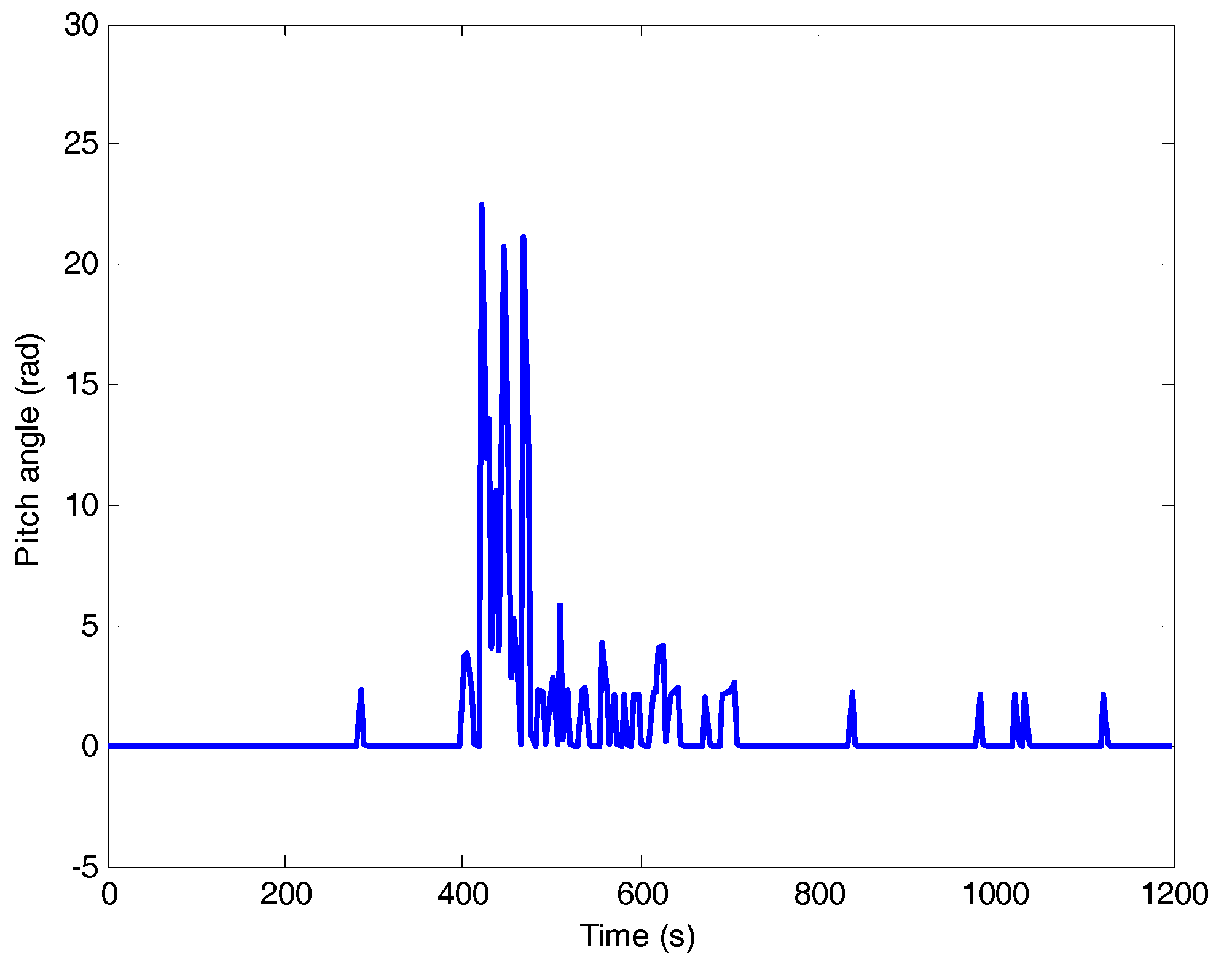
The simulation results based on the wind speed curve shown in Figure 8 are shown in Figure 9, Figure 10 and Figure 11. Table 3 gives the control parameter output average and error for a comparison among the three controllers. The pitch angle change is shown in Figure 9, where β = 0 or > 0 depending on the wind speed fluctuation around the rated wind speed. Figure 10 shows the turbine rotor speed under the operational status. From this figure, it is observed that the PID, conventional sliding mode, and the quasi-continuous second order sliding mode controller can constantly and stably track the rotor speed.

Figure 11 presents the turbine rotor speed error given by the three controllers in pairwise comparison, where the second order sliding mode control gives quite a small error, implying smaller chattering and higher stability. It is also observed that the power output by each controller follows a similar trend but the total energy output with the second order sliding mode method is slightly higher than with the other two control methods. Clearly, the newly designed controller has better performance than PID and the conventional sliding mode controller, as shown in

Table 4. Simulation results of turbine rotor speed, speed error and output power.

Simulation Output	PID	Conventional Sliding Mode	Second Order Sliding Mode
Rotor speed average (rad/s)	1.5113	1.4930	1.5097
Rotor speed std. (rad/s)	0.1513	0.1634	0.1410
Mean absolute error of rotor speed (rad/s)	0.0668	0.0603	0.0066
Std. of absolute error of rotor speed (rad/s)	0.0987	0.0852	0.0508
Sum of square error of rotor speed (rad/s)	7.0027	5.2260	1.1854
Output power average (kw)	840.20	840.35	846.24
Output power std. (kw)	216.44	223.89	219.56

.

5.3. Simulation Scenario 3: Wind Speed Is above the Rated Speed but Less Than the Cut-Out Speed

Under this scenario, the wind speed is in the range from 16 m/s to 22 m/s as shown in Figure 12, for example. The average wind speed is 18.72 m/s and the turbulence intensity is 12%.

The simulation results based on the wind speed as shown in Figure 12 are shown in Figure 13, Figure 14 and Figure 15.

Table 5. Simulation results of turbine rotor speed, speed error and output power.

Simulation Output	PID	Conventional Sliding Mode	Second Order Sliding Mode
Rotor speed average (rad/s)	1.7593	1.7216	1.7467
Rotor speed std. (rad/s)	0.1044	0.0975	0.0778
Mean absolute error of rotor speed (rad/s)	0.0406	0.0647	0.0189
Std. of absolute error of rotor speed (rad/s)	0.1044	0.0975	0.0778
Sum of square error of rotor speed (rad/s)	7.9120	7.3733	4.3565
Output power average (kw)	144.84	143.79	147.79
Output power std. (kw)	165.73	156.03	79.150

gives the control parameter output average and error for making a comparison among the three controllers. The pitch angle change is shown in Figure 13. Figure 14 shows the turbine rotor speed in operation. From this figure, it is observed that the quasi-continuous second order sliding mode controller gives smaller fluctuation of rotor speed than the PID and conventional sliding mode controller. It is clearly shown that the turbine rotor speed error given by the sliding mode controllers is much smaller than the PID controller. That means small chattering and higher stability can be achieved by the second order sliding mode control method.

Figure 15 presents the simulated output power using the three controllers. It demonstrates that the quasi-continuous second order sliding mode controller gives smaller fluctuation of out power than the PID and conventional sliding mode controller. Clearly, the newly designed controller has better performance than PID and the conventional sliding mode controller as shown in Table 5.

In summary, the proposed quasi-continuous second order sliding mode pitch controller has strong robustness under the influence of disturbance and model parameter uncertainty. It can effectively reduce buffeting and the mechanical stress of the system. The effectiveness of the newly designed controller has been well demonstrated using simulation. It is envisaged that it will have certain significance in real application as the turbine rotor speed error is reduced and the output power is improved.

6. Conclusions

A quasi-continuous second order sliding mode pitch controller is discussed in detail in this paper. It also discusses the speed control strategy of the wind turbine in the three wind speed regions, i.e., wind speed is below the rated speed, wind speed is in the range of below and above the rate speed, and wind speed is above the rated speed. The design process of the controller is described and the controller stability is proved. It is verified that the new controller is able to satisfy the wind turbine control requirement in all wind condition.

Under the influence of external disturbance and parameter uncertainty, the proposed quasi-continuous second order sliding mode method is applied to wind turbine pitch control. Based on the simulation results, it is shown that the proposed controller based on quasi-continuous high-order sliding mode can present an optimized control for the wind turbines. It has strong robustness and can effectively suppress the control chattering in all wind speed range, to which the traditional sliding mode control method is ineffective. Based on the simulation results, it can be inferred that the fatigue stress on wind turbine blades is able to be reduced using the second order sliding mode control method than the PID and conventional sliding mode control as the control chattering and the turbine rotor speed error can be clearly reduced. At the same time, the output power is able to be improved especially in higher wind speed region. Given the simulation results shown in Table 5, the average output power generated by the quasi-continuous second order sliding mode control is about 1.5% higher and the output power standard deviation is around 50% reduced than the PID and the traditional sliding mode control in high wind speed region. The next step of the research is to demonstrate the usefulness and effectiveness of the new controller by conducting an on-site trial application to wind turbine pitch control.

References

- Torchani, B.; Sellami, A.; Garcia, G. Saturateci sliding mode control for variable speed wind turbine. In Proceedings of the 5th International Renewable Energy Congress (IREC), Hammamet, Tunisia, 25–27 March 2014; pp. 1–5. [Google Scholar]
- Liu, X.; Han, Y.; Wang, C. Second-order sliding mode control for power optimization of DFIG-based variable speed wind turbine. IET Renew. Power Gener. 2017, 11, 408–418. [Google Scholar] [CrossRef]
- Jafarnejadsani, H.; Pieper, J.; Ehlers, J. Adaptive control of a variable-speed variable-pitch wind turbine using radial-basis function neural network. IEEE Trans. Control Syst. Technol. 2013, 21, 2264–2272. [Google Scholar] [CrossRef]
- Zhang, B.M.; Chen, J.H.; Wu, W.C. A Hierarchical model predictive control method of active power for accommodating large-scale wind power integration. Autom. Electr. Power Syst. 2014, 09, 6–14. [Google Scholar]
- Evangelista, C.; Valenciaga, F.; Puleston, P. Active and reactive power control for wind turbine based on a MIMO 2-sliding mode algorithm with variable gains. IEEE Trans. Energy Convers. 2013, 28, 682–689. [Google Scholar] [CrossRef]
- Xie, J.P. Study on Maximal Wind Energy Capture and Grid Connection of Wind Generator System; Yanshan University: Qinhuangdao, China, 2013. [Google Scholar]
- Boukhezzar, B.; Lupu, L.; Siguerdidjanea, H.; Hand, M. Multivariable control strategy for variable speed, variable pitch wind turbines. Renew. Energy 2007, 32, 1273–1287. [Google Scholar] [CrossRef]
- Van Baars, G.E.; Bongers, P.M. Wind turbine control design and implementation based on experimental models. In Proceedings of the 31st Conference on Decision and Control, Tucson, AZ, USA, 16–18 December 1992; pp. 2596–2600. [Google Scholar]
- Zinger, D.S.; Muljadi, E.; Miller, A. A simple control scheme for variable speed wind turbines. In Proceedings of the Conference Record of the 1996 IEEE Industry Applications Conference Thirty-First IAS Annual Meeting, San Diego, CA, USA, 6–10 October 1996; pp. 1613–1618. [Google Scholar]
- Hand, M. Variable-Speed Wind Turbine Controller Systematic Designs Methodology: A Comparison of Nonlinear and Linear Model-Based Designs; NREL Report TP-500e25540; National Renewable Energy Laboratory: Golden, CO, USA, 1999.
- Moradi, H.; Vossoughi, G. Robust control of the variable speed wind turbines in the presence of uncertainties: A comparison between H-infinity and PID controllers. Energy 2015, 90, 1508–1521. [Google Scholar] [CrossRef]
- Pieralli, S.; Ritter, M.; Odening, M. Efficiency of wind power production and its determinants. Energy 2015, 90, 429–438. [Google Scholar] [CrossRef]
- Taveiros, F.E.V.; Barros, L.S.; Costa, F.B. Back-to-back converter state-feedback control of DFIG (doubly-fed induction generator)-based wind turbines. Energy 2015, 89, 896–906. [Google Scholar] [CrossRef]
- Zong, Q.; Wang, J.; Tian, B.L.; Tao, Y. Quasi-continuous high-order sliding mode controller and observer design for flexible hypersonic vehicle. Aerosp. Sci. Technol. 2013, 27, 127–137. [Google Scholar] [CrossRef]
- Saravanakumar, R.; Jena, D. Validation of an integral sliding mode control for optimal control of a three blade variable speed variable pitch wind turbine. Electr. Power Energy Syst. 2015, 69, 421–429. [Google Scholar] [CrossRef]
- Evangelista, C.; Puleston, P.; Valenciaga, F.; Fridman, L.M. Lyapunov-designed super-twisting sliding mode control for wind energy conversion optimization. IEEE Trans. Ind. Electron. 2013, 60, 538–545. [Google Scholar] [CrossRef]
- Beltran, B.; Tarek, A.; Benbouzid, M. Sliding mode power control of variable-speed wind energy conversion systems. IEEE Trans. Energy Convers. 2008, 23, 551–588. [Google Scholar] [CrossRef] [Green Version]
- Beltran, B.; Tarek, A.; Benbouzid, M. High-order sliding mode control of variable-speed wind turbines. IEEE Trans. Ind. Electron. 2009, 56, 3314–3321. [Google Scholar] [CrossRef] [Green Version]
- Merida, J.; Aguilar, L.T.; Davila, J. Analysis and synthesis of sliding mode control for large scale variable speed wind turbine for power optimization. Renew. Energy 2014, 71, 715–728. [Google Scholar] [CrossRef]
- Zinober, A.S.I. (Ed.) Deterministic Control of Uncertain Systems; Peter Peregrinus Press: London, UK, 1990; ISBN 978-0-86341-170-0. [Google Scholar]
- Qin, B.; Zhou, H.; Du, K.; Wang, X. Sliding mode control of pitch angle based on RBF neural-network. Trans. China Electrotech. Soc. 2013, 28, 37–41. [Google Scholar]
- Levant, A. High-order sliding modes, differentiation and output- feedback control. Int. J. Control 2003, 76, 924–941. [Google Scholar] [CrossRef]
- Levant, A. Quasi-continuous high-order sliding-mode controllers. IEEE Trans. Autom. Control 2005, 50, 1812–1815. [Google Scholar] [CrossRef]
- Hu, Y. The Application of Quasi-continuous High Order Sliding Mode in the Controller Design of Hypersonic Vehicles; Huazhong University of Science and Technology: Wuhan, China, 2012. [Google Scholar]
- Levant, A. Homogeneity approach to high-order sliding mode design. Automatica 2005, 41, 823–830. [Google Scholar] [CrossRef]
- Zhao, W.W.; Zhang, L.; Jing, Y.W. Optimization design of controller for pitch wind turbine. Power Syst. Technol. 2014, 12, 3436–3440. [Google Scholar]
- Abdeddaim, S.; Betka, A. Optimal tracking and robust power control of the DFIG wind turbine. Electr. Power Energy Syst. 2013, 49, 234–242. [Google Scholar] [CrossRef]
- Saravanakumar, R.; Jena, D. A novel fuzzy integral sliding mode current control strategy for maximizing wind power extraction and eliminating voltage harmonics. Energy 2015, 85, 677–686. [Google Scholar]
- Zhou, Z.C.; Wang, C.S.; Guo, L. Output power curtailment control of variable-speed variable-pitch wind turbine generator at all wind speed regions. Proc. CSEE 2005, 35, 1837–1844. [Google Scholar]
- Wang, J.; Zong, Q.; Tian, B.L.; Fan, W.R. Reentry attitude control for hypersonic vehicle based on quasi-continuous high order sliding mode. Control Theory Appl. 2014, 31, 1166–1173. [Google Scholar]
Figure 1.
Different regions of wind turbine operation with wind speed.
Figure 2.
Variable speed control scheme for wind turbine.
Figure 3.
Simplified two-mass model of wind turbines.
Figure 4.
Second order sliding mode simulation model using MATLAB/SIMULINK. (a) Simulation diagram; (b) Simulation diagram.
Figure 5.
Wind speed.
Figure 6.
The turbine rotor speed.
Figure 7.
Turbine rotor speed error.
Figure 8.
Figure 9.
Pitch angle change.
Figure 10.
Figure 11.
Figure 12.
Figure 13.
Figure 14.