Article

Learning-Based Adaptive Imputation Methodwith kNN Algorithm for Missing Power Data

1
Department of Electrical Engineering, Korea Advanced Institute of Science and Technology, Daejeon 34141, Korea
2
Department of Software, Gachon University, Seongnam 13120, Korea
3
Korea Electric Power Research Institute, Daejeon 305-760, Korea
*
Author to whom correspondence should be addressed.
Energies 2017, 10(10), 1668; https://doi.org/10.3390/en10101668
Submission received: 29 August 2017 / Revised: 15 October 2017 / Accepted: 17 October 2017 / Published: 21 October 2017

Abstract

:
This paper proposes a learning-based adaptive imputation method (LAI) for imputing missing power data in an energy system. This method estimates the missing power data by using the pattern that appears in the collected data. Here, in order to capture the patterns from past power data, we newly model a feature vector by using past data and its variations. The proposed LAI then learns the optimal length of the feature vector and the optimal historical length, which are significant hyper parameters of the proposed method, by utilizing intentional missing data. Based on a weighted distance between feature vectors representing a missing situation and past situation, missing power data are estimated by referring to the k most similar past situations in the optimal historical length. We further extend the proposed LAI to alleviate the effect of unexpected variation in power data and refer to this new approach as the extended LAI method (eLAI). The eLAI selects a method between linear interpolation (LI) and the proposed LAI to improve accuracy under unexpected variations. Finally, from a simulation under various energy consumption profiles, we verify that the proposed eLAI achieves about a 74% reduction of the average imputation error in an energy system, compared to the existing imputation methods.

1. Introduction

To efficiently and reliably manage and operate a distributed energy system (DES), which encompasses a diverse array of energy generation, storage, monitoring and control solutions, emerging data from smart meters and other sensors have begun to be accumulated and utilized [1,2]. This massive amount of collected data plays an import role in making a DES intelligent by providing valuable underlying information. Notably, to guarantee reliable and useful information from the collected data, the quality of raw data should be considered prior to refinement of raw data. Here, it is noted that the quality of raw data is measured by the amount of missing values in raw data [3,4]. However, while storing the incoming measurement data in a database, missing values easily can occur due to harsh working conditions or uncontrollable factors, such as malfunctions of devices and imperfect communication signals. This could pose a critical problem when the measurement data are used for real-time control solutions, real-time scheduling for energy trading or a customer service such as a billing system [5,6,7]. Nevertheless, most previous studies related to power data have concentrated on designing a demand forecasting mechanism or robust methods to missing data [8,9,10]. The limitations of these previous research efforts have recently motivated studies focused on handling missing data in energy systems [11,12].
There are two primary methods for handling missing power data in the literature of energy systems. One common imputation method employed in energy systems is to use interpolation with adjacent available measurement data. This approach is very simple, but powerful if the measured data have a consistent behavior or the intervals of missing data are short. However, in the cases of inconsistent behavior or long missing intervals, it will result in low accuracy. Another way is to employ the nearest-neighbor (NN), which uses non-missing data in a certain fixed range around missing points. For example, data collected at the same time the previous week or the following week are used. This is reasonable when the power data have a distinct periodic pattern, and thus, a valid estimated value can be obtained from the fixed range. However, power data will not always have a distinct periodic pattern. Similar to NN, non-parametric regression (NPR) also uses non-missing data selected as useful data for missing data imputation to increase the chance of obtaining a valid estimated value. In an energy system, this methodology can be applied by browsing and utilizing similar load patterns based on the premise that energy data repeat over time with human activities. Although NPR has more complexity compared to interpolation or simple NN, it outperforms the latter two methods when a vast amount of data represents certain patterns. In addition, NPR does not generate a complex model, and it is a promising approach with a massive amount of data [13]; further, some guidelines to handle missing power data in the energy industry are based on the concept of NPR, as well as NN. However, even though a large amount of power data is being generated and this amount will increase, a method that makes use of NPR to estimate missing power data has not been clearly suggested thus far. Recently, by utilizing the correlation between power data, voltage and frequency data of different homes, the authors in [11] newly suggested a novel approach for imputation of missing power data for real-time scheduling in a microgrid. In addition to power data, the work in [11] requires voltage or frequency data for each appliance. Thus, if only the power data of the whole household are collected, this method is difficult to apply, which is a limitation of this work.
On the other hand, in order to efficiently utilize the above methods, in the energy industry, if missing intervals are shorter than one or two hours, the point-to-point linear interpolation (LI) method is applied. In contrast, if missing intervals are longer than one or two hours, the historical average (HA) methods such as NN or NPR are applied for imputation by considering the trade-offs between calculation complexity and imputation accuracy [14,15,16,17,18]. Here are some examples of HA in the energy industry: First, in [16], if the missing interval exceeds 2 h, the missing data are substituted using data of the nearest equivalent day. For instance, missing data on Wednesday can be imputed from the data on last Wednesday, or data from last Tuesday or Thursday can be used unless the data from last Wednesday are available. In the case of public holidays, the nearest Sunday is used as the nearest equivalent day. The work in [18] also considers the meter data of the equivalent day for imputation. The main difference with [16], which imputes missing data from a single equivalent day, is to select three equivalent days and impute the missing data from the average value of those selected three values. The use of LI and HA is reasonable if we assume that small or consistent variations only exist in one or two hours or less. Nevertheless, there is still a high possibility for large or inconsistent variations to occur even in short intervals (e.g., two hours or less), and thus, this assumption is not always satisfied. In this sense, the LI results in poor performance of imputation even in short missing intervals. Accordingly, method selection criteria based only on fixed missing interval lengths without considering each load pattern cannot optimally be adapted to unpredictable variations in the energy system. Recently, to resolve this issue, Peppanen et al. in [12] suggested an optimally-weighted average (OWA) data imputation method. The work in [12] imputes missing data with a weighted sum of LI and their own HA. In addition, this method employs an optimal weight factor to enhance the imputation performance. However, since they aim to impute missing data with available data in a fixed time range (e.g., +8–−8 days and +1 and 1 times), it requires the strong assumption that non-missing data within this fixed range provide valid estimated values for missing data. Moreover, because the proposed optimal weight factor depends on missing intervals, it is seriously affected by LI at a short missing interval. In addition, as they also refer to some collected data after the missing data, it is difficult to apply this approach to instant imputation for real-time applications in an energy system. Thus, the previously proposed work in [12] still has shortcomings that should be addressed, and this is the inspiration for the present work.
In this paper, we propose a novel learning-based adaptive imputation method (LAI) that imputes missing power data by browsing and utilizing similar load patterns from past situations. Here, to represent a past situation from power data, we model feature vectors by using past data and their variations. Furthermore, the optimal length of the feature vector and the optimal historical length for imputing missing power data are decided in the learning process. Finally, the missing power data are estimated by referring to the k most similar past situations in the optimal historical length. Furthermore, we extend our proposed LAI to alleviate the effect of unexpected variation in power data and refer to this approach as an extended LAI method (eLAI). The eLAI then further improves the accuracy by selecting a method between LI and the proposed LAI. In addition, since the proposed methods impute missing data immediately after the first succeeding non-missing data arrive, it is not necessary to refer to future data; they are therefore suitable for the application to situations where instant imputation is needed. We verify that the proposed eLAI achieves about a 74% reduction of average imputation error in an energy system, compared to the existing methods.
The contributions of this paper are summarized as follows.
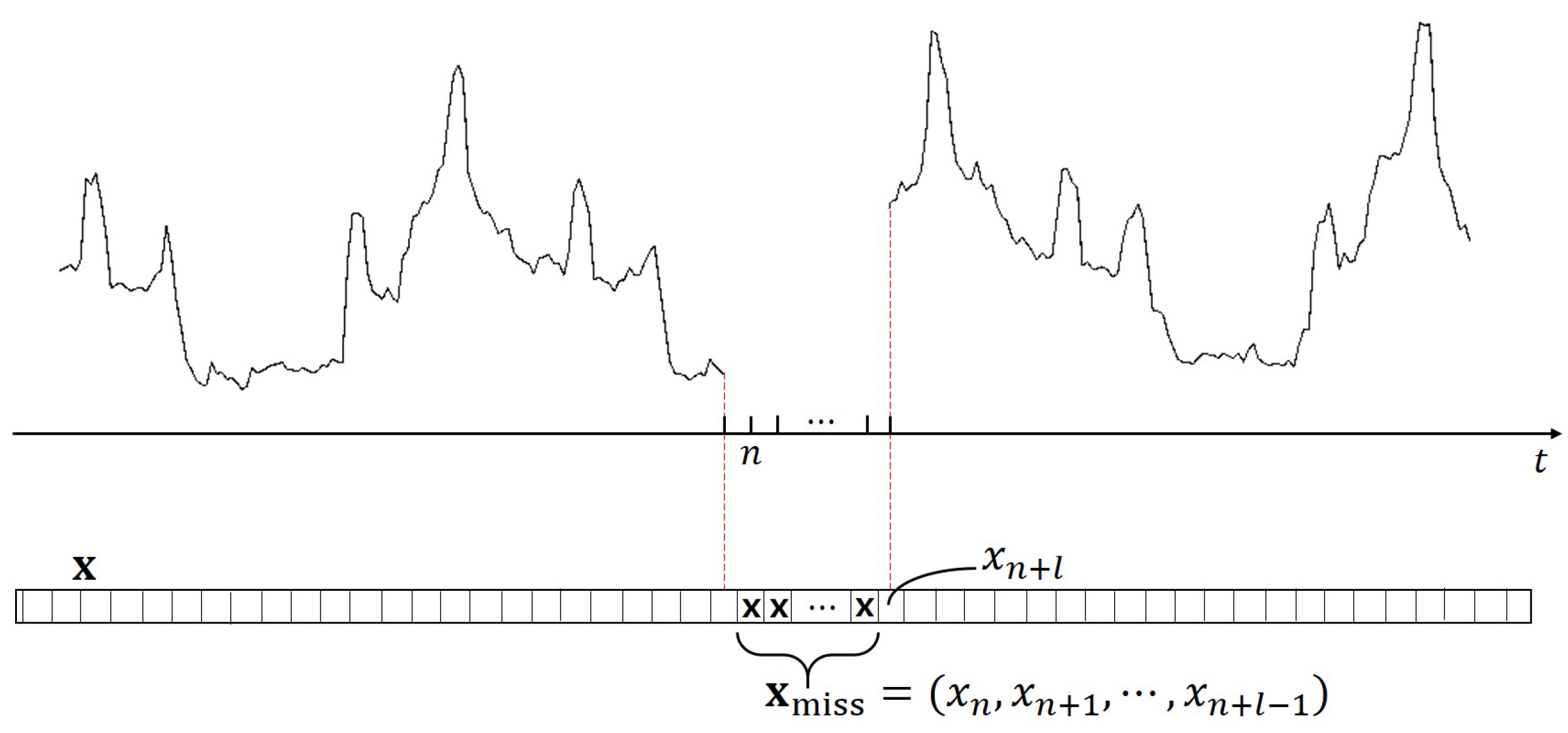
  • A novel feature vector is modeled for representing the patterns of past power data under an NPR-based model for missing power data imputation.
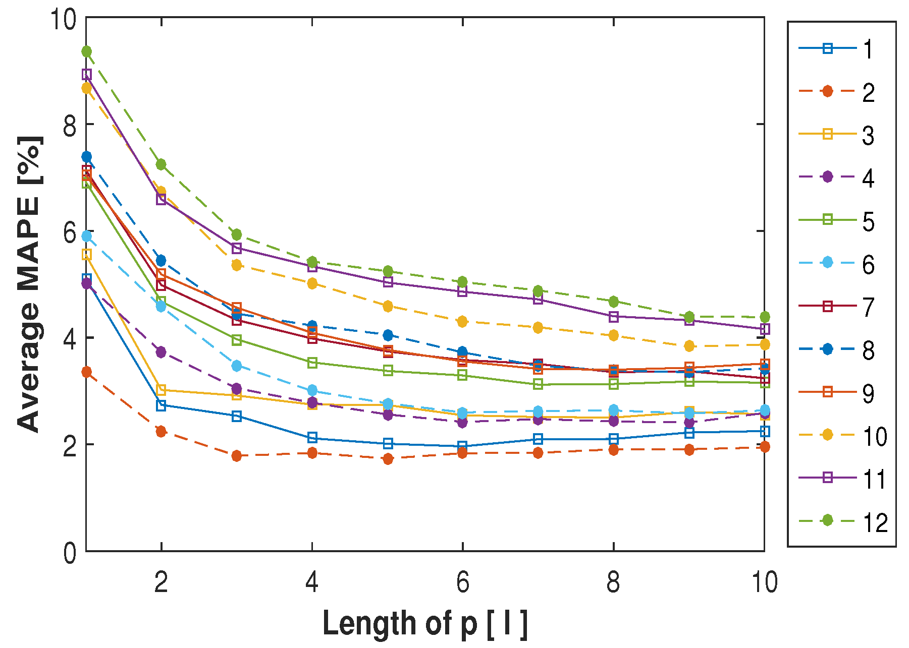
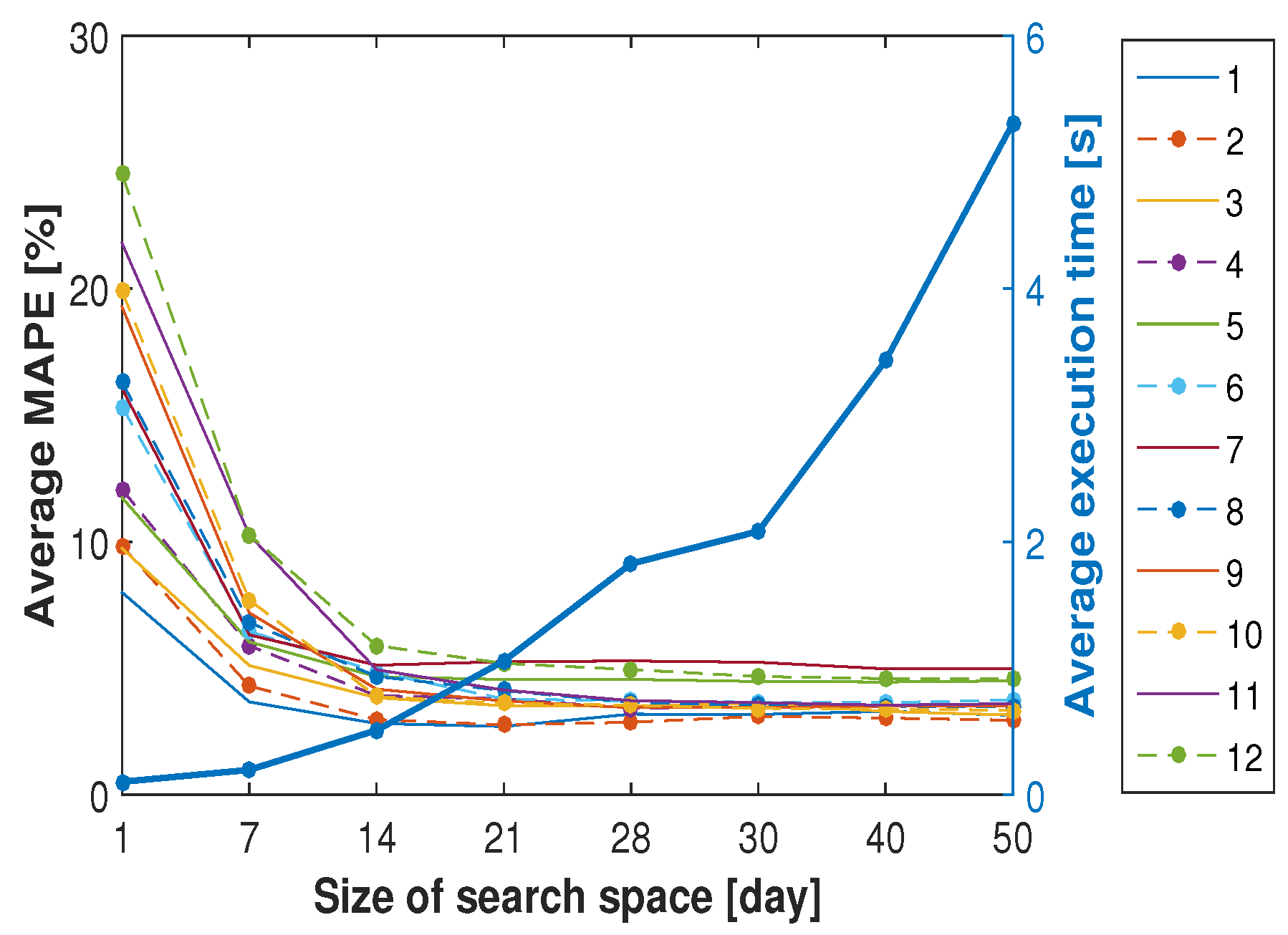
  • Through learning, the optimal length of the feature vector and the optimal historical length are decided. Furthermore, the proposed LAI imputes accurate missing power data by using a weighted distance within an optimized historical length.
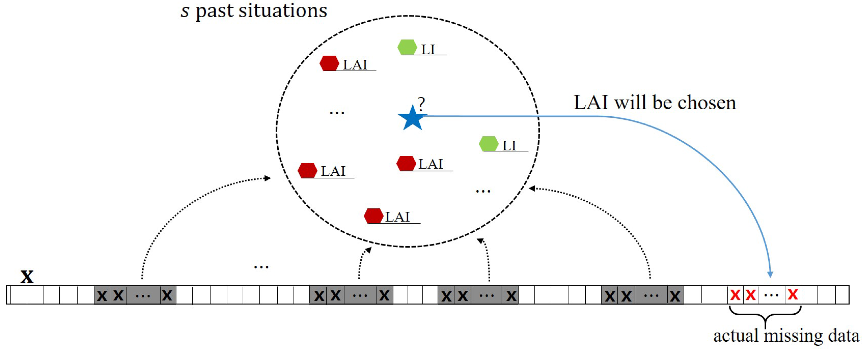
  • The proposed method is extended to improve the accuracy of missing data imputation considering an unexpected variation of power data by adaptively selecting between LI and the proposed LAI.
  • From the simulation under various energy consumption profiles, the proposed method is analyzed and validated. Finally, the proposed eLAI achieves about a 74% reduction of average imputation error in an energy system, compared to the existing methods.
This paper is organized as follows. The proposed method is explained in detail in Section 2. In Section 3, the performance evaluation with various missing lengths and missing ratios is discussed. Two significant hyper parameters of the proposed method and future work are discussed in Section 4. Finally, the conclusion of this paper is provided in Section 5.

2. Learning-Based Adaptive Imputation Method

We consider that meter data are collected periodically (e.g., 15 min), and when there is missing data, imputation is conducted immediately after the first succeeding available data are observed. Let x t be the observed power data at time index t { 1 , 2 , } where the one-dimensional vector x represents the collected data vector. Then, as illustrated in Figure 1, if missing data occur during the missing interval l with the first missing data at t = n , the missing data are estimated as x miss = ( x n , x n + 1 , , x n + l 1 ) immediately after the first non-missing data x n + l arrive. Here, the proposed method aims at generating an accurate x miss vector.

2.1. Proposed LAI Method

The proposed LAI imputes a missing power data by browsing and utilizing similar load patterns from past power data. Here, by using this past power data as input data, the optimal length of the feature vector and the optimal historical length for imputing missing power data, which are significant hyperparameters of the proposed LAI, are decided in the learning process. Finally, missing data are estimated by referring to k most similar past situations in the optimal historical length.
Let the time index at which the data loss occurred be zero and x 0 = ( x p , , x 1 , x 0 , , x l 1 , x l ) denote the missing situation. The missing situation contains p previous data ( x p , , x 1 ), one first succeeding datum ( x l ) and l missing data ( x 0 , , x l 1 ). The former two, p previous data and the first succeeding data, denote surrounding data of the missing situation, x 0 surr = ( x p , , x 1 , x l ) , and the last one denotes missing data, x 0 miss = ( x 0 , , x l 1 ) . Moreover, these representations are applied to define the past situation. Thus, the first past situation is denoted by x 1 = ( x p 1 , , x 2 , x 1 , , x l 2 , x l 1 ) . Likewise, x 1 is decomposed into x 1 surr and x 1 miss representing the surrounding data of the first past situation and the data corresponding to x 0 miss . It should be noted that x 1 miss is the past power data used for imputation, while x 0 miss is the actual missing data. The proposed LAI then browses and utilizes past situations x 1 x t max for imputing x 0 miss in x 0 . Here, a past situation has the index set P = { 1 , 2 , , t max } where t max , which is called the historical length, is the maximum number of past situations for imputation. Figure 2 illustrates an example of a missing situation, the first past situation and the last past situation with historical length t max . In each situation in Figure 2, the shaded area represents the surrounding data, and the area with mark X represents the missing data.
In order to model a past situation used for imputation, we newly define the feature vector that contains not only the values of surrounding data ( x i surr ), but also the information on the variation ( x i surr ) to best reflect the pattern of situations. Here, x i surr is given as follows, and the index n represents each data point in x i surr and x i surr .
x i surr [ n ] = x i surr [ n + 1 ] x i surr [ n ] , n { 0 , , p 1 } .
The feature vector is then defined by f i = ( x i surr , x i surr ) , i { 0 } P . f 0 denotes the feature vector of the missing situation, and f i , i P denotes that of the i-th past situation. Here, care is taken not to use feature vectors of past situations that include missing entries. For example, if there are any missing data in a feature vector, this feature vector is excluded.
Next, the distance between f 0 and f i is calculated for choosing the k most similar past situations. This is based on the idea of the kNN algorithm. At this time, a linear weight to each point of the feature vector is used based on the time distance from the missing data point. This means that the closer the value is to the missing point, the greater the significance is when we find past similar situations to a missing situation. w is a linear weight matrix whose diagonal entries are given by { 1 , 2 , , p , p , 1 , 2 , , p 1 , p 1 } with other entries zeros, and d i is a weighted distance between f 0 and f i , given by:
d i = ( f i f 0 ) w ( f i f 0 ) T ,
where:
w = 1 0 p 1 0 p 1 .
Finally, the missing data are imputed as follows. Note that J = { n 1 , n 2 , , n k } is the index set of the selected past situation. The actual missing data x 0 miss are then filled with the weighted summation of x j miss , j J , using a weight in inverse proportion to the square of d j . Thus, imputed data, which are denoted by x LAI , are calculated by the following equation. Here, 1 miss and 1 surr are one-by-l and one-by- ( p + 1 ) vector of one, respectively.
x LAI = j J ( x j miss + c j · 1 miss ) d j 2 / j J d j 2 ,
where the compensation factor c j is the difference between the missing and past situations to improve the accuracy, such that:
c j = 1 p + 1 ( x 0 surr x j surr ) · 1 surr .
In the proposed LAI, the length of the feature vector (p) and the historical length ( t max ) impact the imputation accuracy, as well as the complexity. Specifically, p relates to how well a situation is described to find more similar past situations and t max relates to how similar past situations are found. Due to a trade-off relationship between the accuracy and the complexity of the proposed LAI, it is important to decide appropriate values for them. Hence, these parameters should be carefully decided. On the other hand, k, a parameter of the kNN algorithm, also has a critical effect on the performance of the kNN algorithm. If the value of k is too large, it may lead to a large model bias. Conversely, if the value of k is too small, the model would become too sensitive to outliers. Therefore, k also should be carefully chosen as an appropriate value. The general approach to choose the value of k is conducted by measuring the error on the training data and picking a value that gives the best generalization performance [19]. As such, the method of selecting p and t max is also similar to the process in which k is selected considering the bias and the variance of the kNN algorithm. Correspondingly, we design a learning method to find the optimal length of the feature vector (p) and the optimal historical length ( t max ), as presented in Algorithm 1. In this algorithm, n intentional missing situations are generated to learn the optimal p and t max . At this step, n intentional missing situations can be understood as a training dataset to find optimal p and t max . Then, as both the p and t max increase, each n intentional missing datum is estimated, and the average imputation error of this missing datum is calculated. If the current calculated error is less than the error calculated from the previous p and t max , the optimal hyper parameter value is updated to the current p and t max . Furthermore, if the difference between the previous error and the current error converges to the pre-defined threshold value, the learning process is completed and returns the current p and t max as optimal values.
Algorithm 1 Learning algorithm for optimal p and t max selection.
INPUT:
M = { m 1 , m 2 , m n } (set of intentional missing situation),
P, T max , initial error, error condition
OUTPUT: p , t max
1:
procedure optimal p and t max
2:
    error = initial error
3:
 
4:
    for all p { 1 , , P } and t max { 1 , , T max } do
5:
        for all m i do
6:
           calculate m LAI
7:
        end for
8:
 
9:
        if |average error over M - error| < error condition then
10:
           return p and t max
11:
        end if
12:
 
13:
        if average error over M < error then
14:
           error = average error over M
15:
            p = p
16:
            t max = t max
17:
        end if
18:
 
19:
    end for
20:
end procedure

2.2. Extended LAI Method

In the proposed LAI, k past situations, which have the most similar pattern to the missing situation, are used. This is based on the assumption that collected power data tend to have a similar pattern over time with human activities, as used in the literature [8]. This assumption, however, may not be satisfied under the unexpected variation in the missing interval. This means that there can be an unexpected variation in missing intervals, which differs from past situations despite there being a similar pattern in surrounding data. Here, to alleviate the impact of this unexpected variation, we extended the proposed LAI as the extended LAI method (eLAI), which adaptively selects between LI and the proposed LAI. The procedures of eLAI consist of the following two steps.
Step 1: Similar past situations are selected for deciding the imputation method. In this selected past situations, intentional missing data corresponding to the actual missing data are made and estimated through LI and LAI. Therefore, as LAI finds k similar past situations for missing power data imputation, s past situations that have high similarity to the missing situation are selected.
Step 2: Intentional missing data are estimated for each s selected past situations by using two methods, LI and LAI, and the results of the two methods are compared in terms of imputation accuracy for each s past situation. Then, one method is selected by a majority vote of s results, and one selected method is finally used for the actual missing data imputation. Figure 3 illustrates the procedure of eLAI. In Figure 3, the results of estimating the intentional missing power data for each s past situations show that the LAI will be more accurate than when using LI, and consequently, LAI is selected for the actual missing data imputation.
In this way, eLAI not only utilizes historical data, but also the information on the method with better results in similar past situations through intentional missing data. By using another piece of information that can describe the actual missing situation, eLAI alleviates the effect of unexpected variation of the actual missing data on missing data estimation.

3. Performance Evaluation

We evaluate the proposed LAI and eLAI by comparing them to existing methods, LI and OWA [12], which are commonly used or suggested for missing power data imputation. In addition to two comparison methods, the probabilistic principle component analysis (PPCA)-based imputation method, which had been proven to be one of the most effective imputing methods in traffic data [20,21], is also compared. In this evaluation, various missing lengths and missing ratios are considered, and all missing data are intentionally generated with these missing lengths and missing ratios. The performance is measured by the mean absolute percent error (MAPE) and the root mean square error (RMSE). The well-known metrics to evaluate the accuracy of imputation, MAPE and RMSE, are defined as follows [12,13]:
MAPE = 100 l t = 1 l | x t real x t est | x t real [ % ] , RMSE = 1 l t = 1 l ( x t real x t est ) 2 ,
where x t real and x t est denote the actual data and the estimated data at time t, respectively.

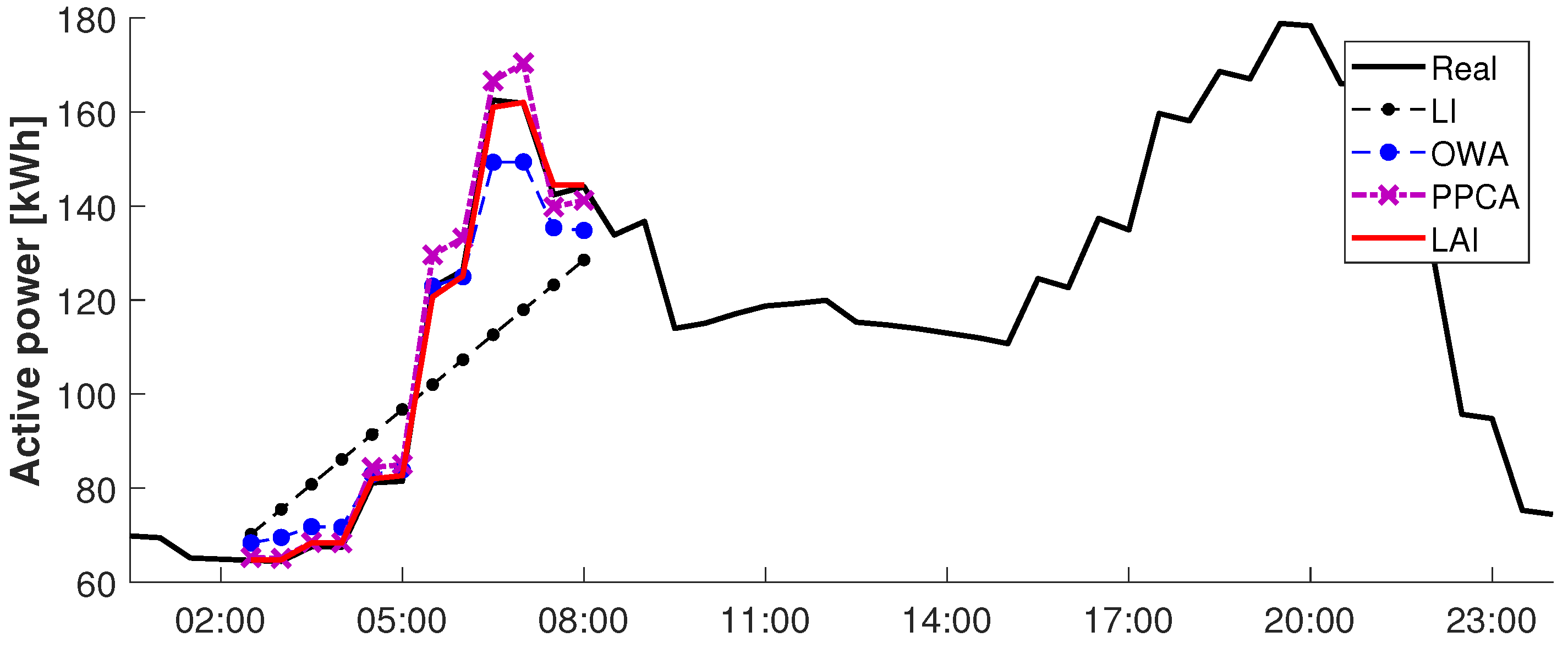
3.1. Comparison Method
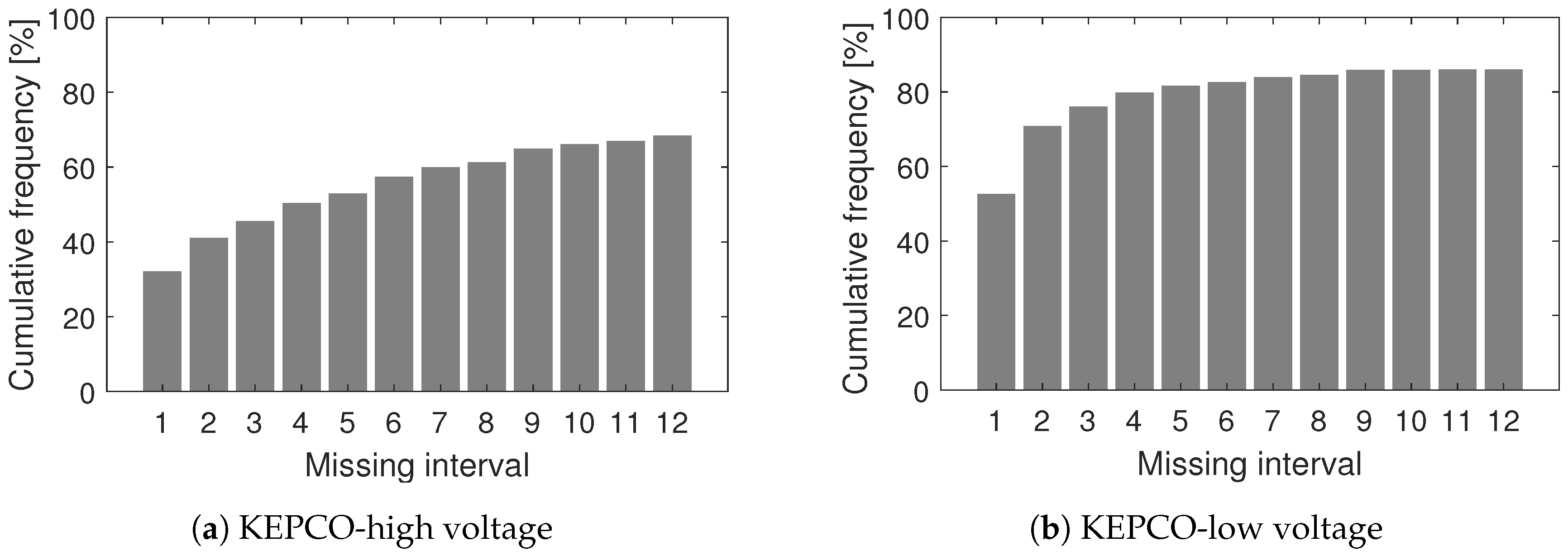
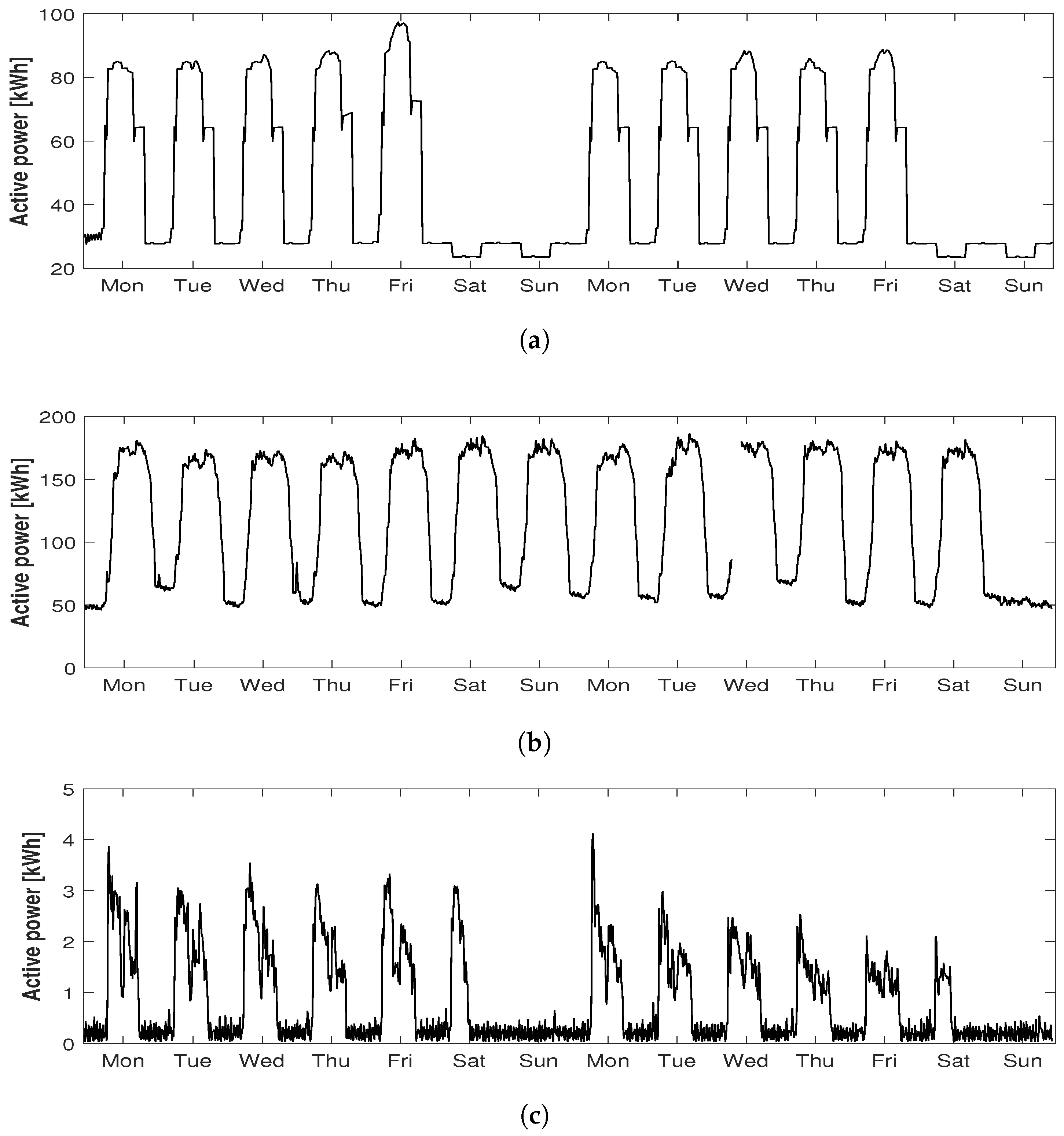
In this subsection, PPCA-based imputation is described briefly. It should be noted that PPCA is based on PCA, which is well known for feature extraction. Specifically, PCA provides principal components of each data where the principal component is the projection of each data into the space of the principal axes. Here, this principal axes maximizes the variance of the data in the projected space. Additionally, the principal axes, which are computed as eigenvectors of the dataset’s sample covariance matrix, represent the distribution of the given dataset. On the other hand, PPCA introduces the probability model for finding principal axes and principal components of the dataset so that both of them can be found even when missing data exist. That is, PPCA can be considered as a maximum-likelihood reformulation of PCA [20,22]. Therefore, PPCA is applied to missing data imputation using principal axes and principal components found from non-missing data inversely. In this performance evaluation, data from the time the data loss occurred up to 21 days ago was used for PPCA-based imputation.

3.2. Data

For the evaluation, two types of data were used. The first one is meter data simulated for the U.S. Department of Energy (DOE) commercial buildings, such as offices, hotels, restaurants and schools over 17 years (1998–2014) for 15 sites in the continental U.S. The time unit of the data is 30 min, and the data are published at the Open Energy Information (OpenEI) [23]. Figure 5a shows an example of one power consumption datum among 45 different buildings.
The second dataset is meter data collected by Korea Electric Power Corporation (KEPCO). At KEPCO, the types of electricity supply are divided into residential, general, educational, industrial and agricultural, depending on the application, and each type is divided again into high (H) and low (L) voltage based on the supply voltage. Among these, the general type includes the electricity supplied to commercial office buildings and some of the electricity for residential, industrial and agricultural types, according to the stipulations of the electricity supply contract, excluding the remaining categories. In this paper, we used general H and L active power data collected from 1 January 2015–10 August 2016 (H) and 16 February 2014–10 August 2016 (L) in the Gwangju area of Korea. The measurements from 1000 (H) and 700 (L) smart meters are recorded every 15 min. From the actual measured data, we can see the following two facts. First, it is observed that 13.34% (H) and 11.60% (L) of the total data are missing. Second, the missing data for up to three hours (i.e., missing interval 12 in this dataset) account for about 68.3% at H and about 85.9% at L. Histograms of the cumulative frequency distribution of missing data depending on the missing interval are shown in Figure 4a,b. Figure 5b,c shows examples of power consumption data actually measured. Furthermore, Figure 6 shows examples of meter data collected on every Monday for one year in each dataset. As can be seen in Figure 6, the real meter data have much more diverse patterns than the simulated data despite the same day of the week, and pattern irregularity in the real meter data seems large. This makes missing data imputation of the real meter data more difficult. In this performance evaluation, reflecting the frequency distribution of real missing data, the missing length ranges from 1 to 12. The missing ratio ranges from 1 to 30%, to observe the robustness of the proposed method across various missing ratios.

3.3. Parameter Selection

Prior to performance evaluation, the parameters of the proposed algorithm (i.e., k, s, p and t max ) were determined as follows. First, 500 intentional missing situations for each missing length were randomly selected in each dataset as training data for parameter selection. This is to reflect diverse and large amounts of power consumption data. Here, one missing situation is a random ordered pair; (smart meter ID, time where intentional data loss occurred). For example, Figure 7 shows an example of the training dataset when the missing interval is three. Then, these parameters are selected based on the measured error in the missing power data imputation performed on the value of the parameter within the appropriate range. Table 1 shows the heuristically optimized k and s in the first dataset. In the second dataset, k is three and s is nine for all missing lengths. Next, heuristically optimized p = 2 l , t max = 21 days were used in this performance evaluation.

3.4. The Result of the Performance Evaluation

The accuracy of the proposed methods were compared to LI, OWA and PPCA with respect to missing intervals in terms of MAPE and RMSE. Figure 8 and Figure 9 show the average MAPE and RMSE with the 95% confidence interval over 1000 random test cases for each missing interval. One test case is a randomly selected intentional missing situation as in parameter selection (smart meter ID, time where intentional data loss occurred). These randomly selected test cases reflect various missing situations. They are independent of the missing situations used in parameter selection.
First, the MAPE and RMSE measured in the first dataset with distinctly repeated patterns as simulated data are shown in Figure 8a and Figure 9a. In this dataset, the missing ratio is 0%, and missing data during from a minimum of 30 min to a maximum of 6 h were estimated. In Figure 8a and Figure 9a, we note that the eLAI shows the lowest average MAPE, RMSE and the shortest 95% confidence interval in most missing length. PPCA also showed relatively accurate imputation results. On the other hand, naturally, the longer the missing interval, the more MAPE and RMSE of LI increased. OWA, which imputes missing values by calculating the weighted sum of estimated values of LI and HA, also increases the error rate as the missing interval becomes longer. Specifically, in this dataset, the proposed eLAI improves about 74.4%, 60.8% and 14.5% average MAPE compared to LI, OWA and PPCA, respectively. In addition, these was about a 3.2% improvement compared to the proposed LAI. In the sense of average RMSE, eLAI achieves about 69.8%, 59.2% and 20.0% improvement over LI, OWA and PPCA and about a 1.1% improvement over LAI. Furthermore, Table 2 and Table 3 show the results of LAI and eLAI when information on the variation is used or not for the feature vector. In most cases, the measured errors with no information on the variation are larger than the values with the information on variation. This result indicates that the accuracy of missing data imputation can be improved when the slope information is included in the feature vector.
Next, the MAPE and RMSE measured from the real meter data are shown in Figure 8b,c and Figure 9b,c. Each was measured in H and L, respectively. In this dataset, missing data during a minimum of 15 min to a maximum of 3 h were estimated. In these figures, we could see at a glance that the results of the second dataset are very different from the first dataset. This is due to the fact that the interval of the measurement time is shorter than the simulated data, the missing ratio of the real meter data is about 10%, and it has very diverse and irregular patterns. First, the overall MAPE of H and L is compared. In most imputation methods, the average MAPE at L is about 1.6-times higher than H. This means that the estimation of the missing data at L is more difficult than the estimation at H. Second, in most of the cases of Figure 8b,c, MAPE of OWA is larger than MAPE of LI. As mentioned before, OWA imputes missing data by calculating the weighted sum of LI and HA. If a missing length is short, OWA is affected by LI, and if the missing length is long, it is affected by HA. Therefore, at this time, a larger error than LI means that HA accuracy is very low, which is again caused by unpredictable characteristics of the real meter data. Furthermore, it can be seen that PPCA shows a very high error rate. Here, PPCA also uses data from the time the data loss occurred up to 21 days ago for comparison with the proposed methods. Under this same condition, PPCA showed good performance in the first dataset, but did not in the second dataset. It can be understood that it is difficult to find latent variables in the second data by only 21 days of data. On the other hand, the proposed eLAI shows the lowest error rate in most cases even in this dataset, which is likely to have unexpected patterns, although the proposed LAI shows some inaccurate estimates compared to other comparison methods.
From these results, it can be verified that the proposed methods estimate the missing power data more accurately than the existing methods. Especially, the proposed eLAI estimates the missing power data accurately in both datasets. In the case of the confidence interval, the length of the eLAI is shorter than the comparison methods. This indicates that the proposed algorithm can perform more reliable imputation. Table 4 shows the overall average of MAPE and RMSE measured in each method. Figure 10 shows an example of missing power data imputation using four methods. Since eLAI selects one of LI and LAI, the chosen method is replaced by eLAI in this figure. These are the results of estimating 12 missing data. As seen in Figure 10, in the case of eLAI, it is seen that LAI is well selected between LI and LAI as an imputation method in this time period, and it is highly accurate compared to the existing methods.

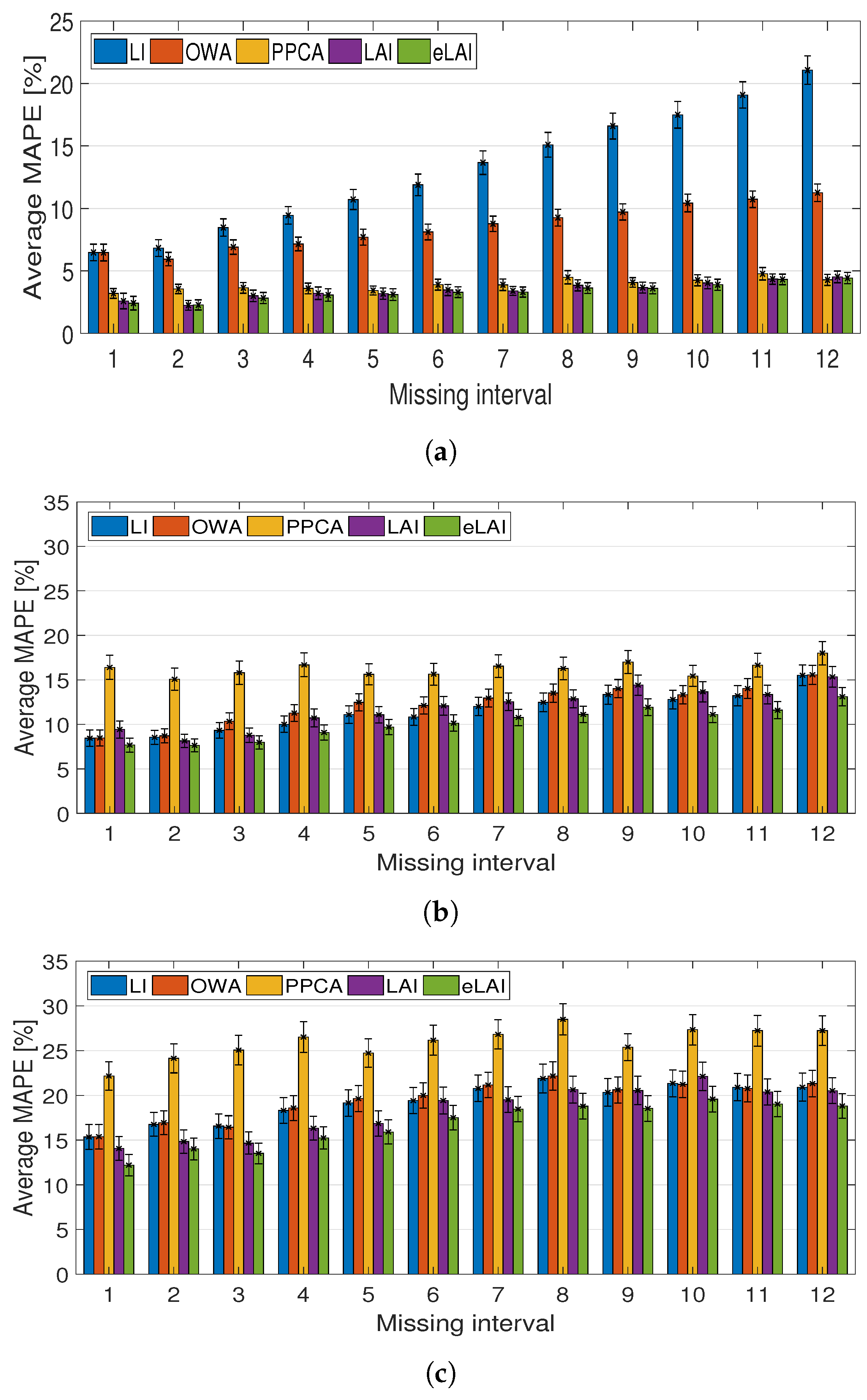
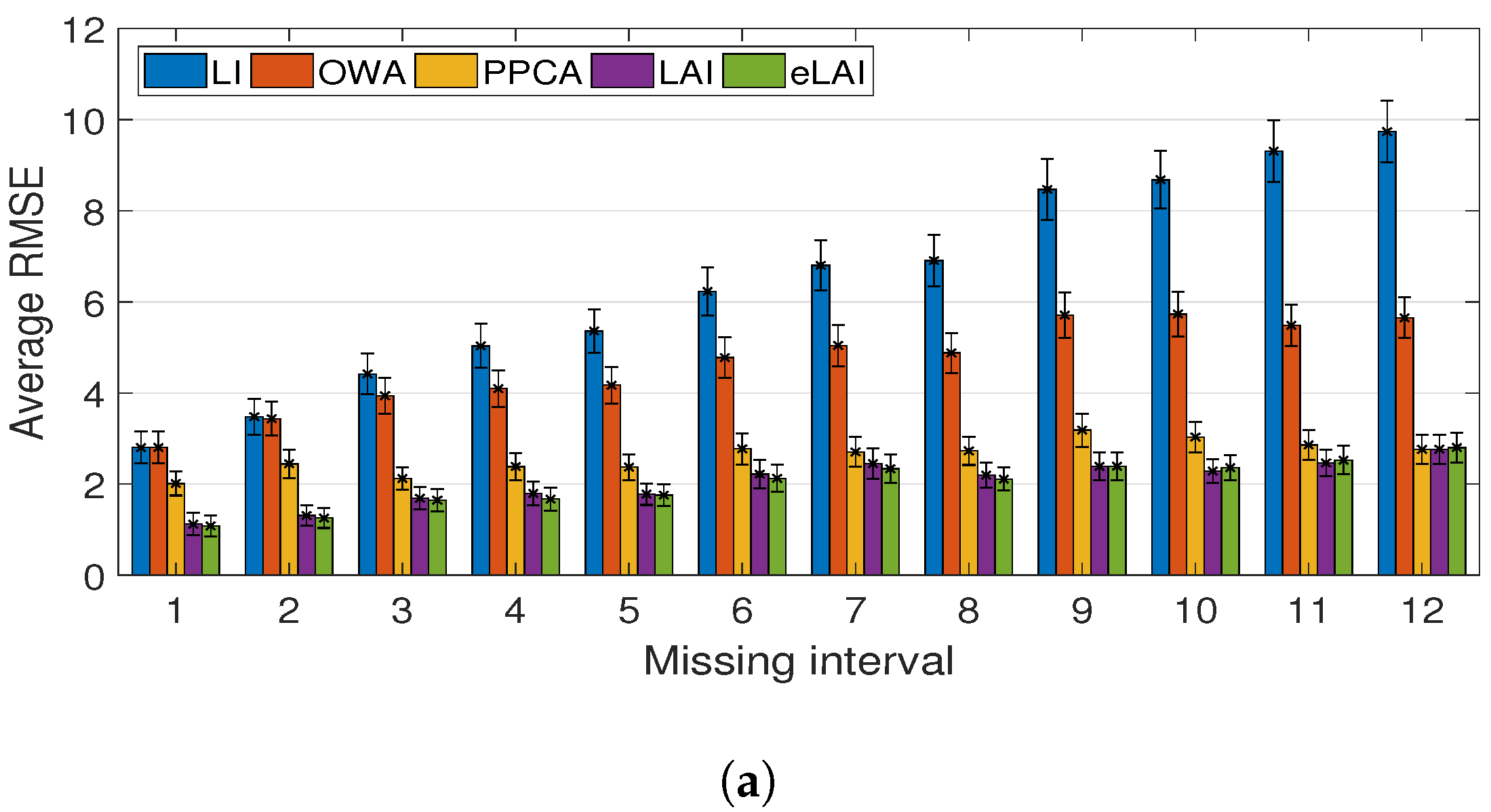
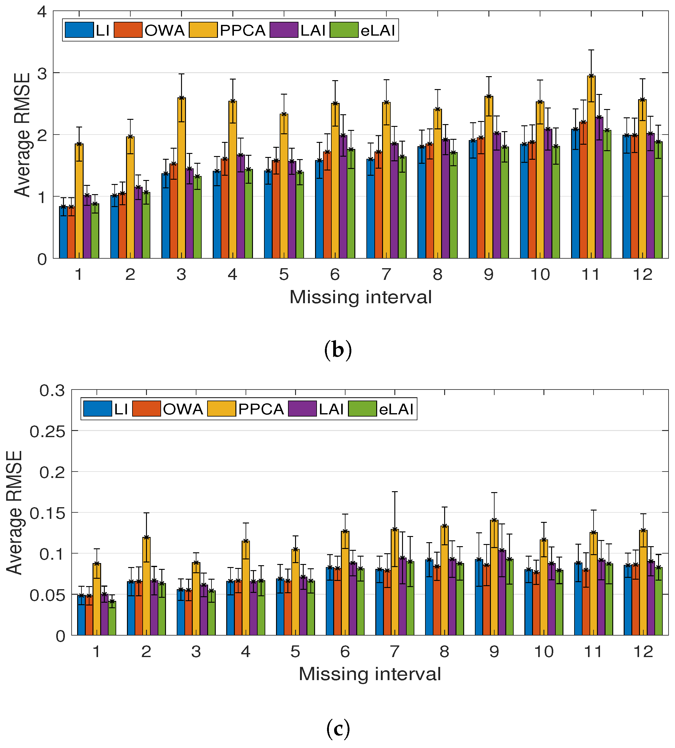
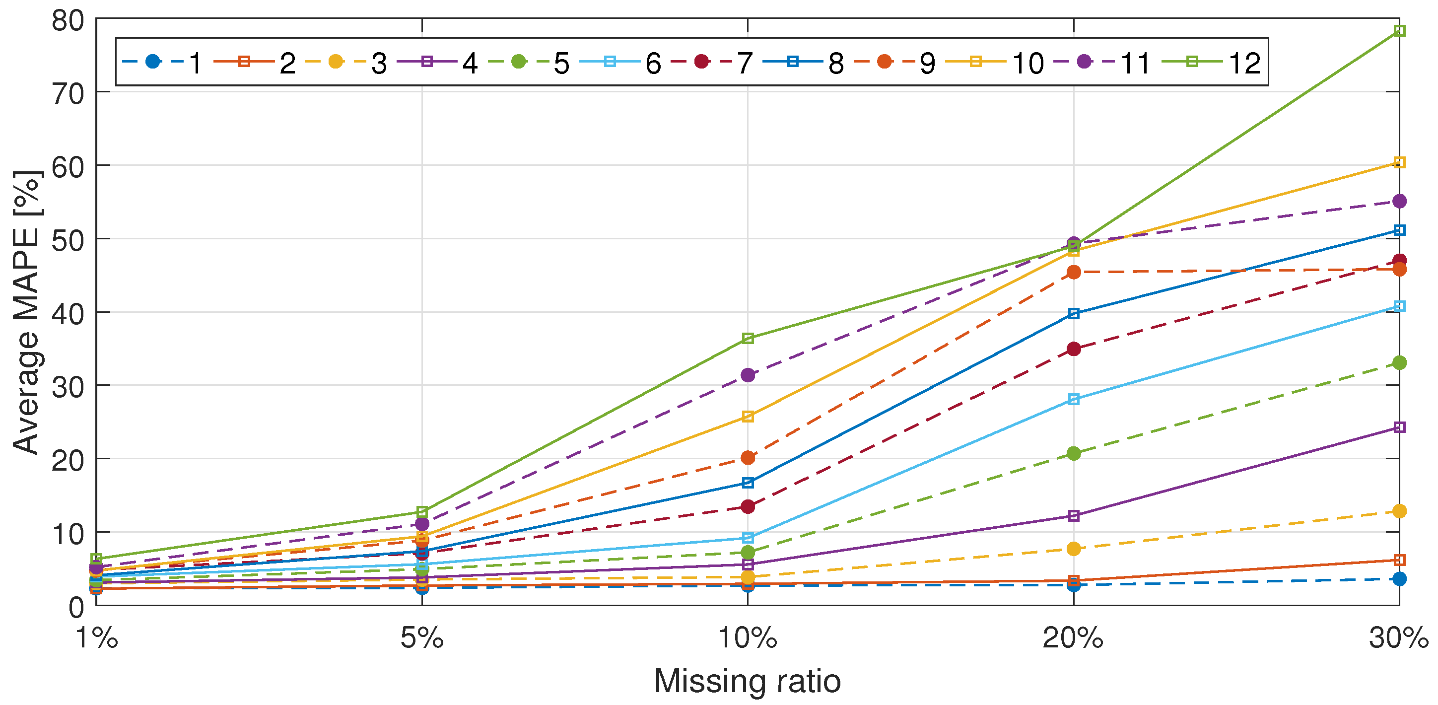
3.5. Performance Evaluation According to the Missing Ratio

Next, a performance evaluation of the proposed eLAI is performed according to the missing ratio with the first dataset. For each test case randomly selected, this algorithm is applied after missing data by the missing ratio in corresponding historical data as shown in Figure 11. Because the proposed eLAI uses historical data, the missing ratio is an important factor affecting performance. As shown in Figure 12 and Table 5, as the missing ratio increases, the error rate and the confidence interval also increases. In particular, the increase in average MAPE was most prominent at the 10–20% missing rate. In addition, at some point of the high missing ratio of historical data, performance analysis cannot be conducted for each missing length, as shown in Table 5. This is a limitation from using the complete past situation for missing data imputation. A discussion on this limitation is also included in Section 4.

4. Discussion and Future Work

This section contains the discussion on the impact of two hyperparameters (i.e., p and t max ) used in LAI, the limitations of the proposed methods and future work to improve it. First, Figure 13 shows the average MAPE over 500 random test cases for each missing length according to the p values. At all missing lengths, the larger the p value, the lower the MAPE is obtained. This means that when searching for similar past situations, the more data that are used to generate a feature vector, the more accurate the missing data estimation will be. However, there is also a case where the MAPE increases when the p value increases, especially at a short missing interval. This is due to fact that if there is an unexpected variation in the missing interval, a larger p value cannot guarantee a more accurate estimation. Next, the value t max is observed. The average MAPE over 500 random test cases for each missing length when the value of t max is increased as in the previous one day, 1 week, 2 weeks and 3 weeks is shown in Figure 14. As seen in this figure, the error rate decreases sharply every time as the historical length increases by one week. However, if the historical length exceeds about three weeks or four weeks, the error rate tends to converge to a constant value. This means that there is an optimal historical length at this convergence point. Beyond this optimal point, the increment of historical length only leads to a longer execution time without any improvement of the error rate, as shown in Figure 14, where the execution environment was Inter(R) Xeon(R) CPU E3-1230 v3 @ 3.30 GHz. The heuristically-optimized hyperparameters in LAI help to find useful historical data for missing data imputation, contributing to accurate estimation and computational efficiency.
However, since the proposed LAI is based solely on historical meter data, we can consider two situations where its performance is rather poor. First, the proposed methods may be degraded when historical data are lost extensively, as seen in Section 3.5. This leads to an inaccurate imputation because it is difficult to detect similar and complete past situations. However, this problem might be also a critical issue for other imputation algorithms, especially learning-based algorithms. In order to improve these problems, it is essential to develop an imputation method that utilizes not only power consumption, but also other environmental variables (weather, occupancy rate, etc.).
Second, suppose we have found several past situations similar to the missing situation using the surrounding data. However, in a situation that corresponds to the actual missing data, there may be situations with unpredictable power consumption patterns. Although eLAI has been proposed to alleviate this problem, unpredicted variation still leads to an inaccurate missing data imputation. Figure 15 shows some cases corresponding to this situation. Figure 15 illustrates intentional missing data, imputed data and the past situation selected based on the similarity of surrounding data. The surrounding data of the selected past situation show a pattern similar to the surrounding data of the missing situation. However, some past situations in Figure 15a,b show a completely different pattern from the real missing data. Conversely, in Figure 15c, the real power consumption data show a different pattern from the selected past situations. In these cases, missing data imputation will result in a large error with the actual value. This is because the past situation selected for imputation contains the unpredictable power consumption in the time corresponding to the actual missing data. The problem of unpredicted patterns of selected past situation can be improved by the following two improvements of the proposed methods: (1) how to select historical data to be used and (2) how to utilize selected historical data.
First, when choosing past data to use for imputation, we can introduce a method to consider similar past situations with incomplete data; or a method considering attribute that can be define through environmental variables in each situation as [24] may be considered. The second is an improvement on how to use selected historical data. Considering the unpredictable power consumption in the selected historical data as one outlier, it is possible to introduce a learning technique such as SVR, which is robust to these outliers [25,26,27]. For example, Figure 15d shows the example of missing data imputation using basic SVR in the same situation as Figure 15b. There is still an error, but it may be less affected by the unexpected pattern in the past situation than in LAI. This shows the room for improvement of the proposed algorithm and becomes the future work of this paper.
Finally, in this paper, it is stipulated that the situation where imputation is necessary is when the first non-missing meter data come in. This is because if the missing data are interpolated as soon as it occurs, it is a kind of a prediction, not an imputation. However, this situation would be important for user-oriented applications (e.g., real-time demand management, smart-metering service, etc.). It should be noted that even in LI, it is not able to perform missing data imputation in such a situation. Nevertheless, in the proposed scheme, by slightly modifying the proposed scheme, it is able to interpolate data without using the first succeeding non-missing data. Specifically, in the similar pattern search step of the proposed algorithm, only the data before the missing interval can be used for the interpolation. Table 6 is the numerical results using the modified algorithm. In this case, MAPE was somewhat higher than that of the conventional LAI or eLAI, but there is no significant difference when compared with other methods.

5. Conclusions

In this paper, we proposed a learning-based adaptive imputation method (LAI) for missing power data. In detail, the proposed LAI estimates the missing power data regardless of missing intervals by using the pattern of power data. To this end, we modeled a feature vector to represent a situation, and the optimal length of the feature vector and the historical length are decided through a learning process. Furthermore, a mechanism to consider unpredicted variation in power data is suggested as an extended LAI (eLAI). In the proposed eLAI, the optimal imputation method is adaptively selected, which also contributes to the accuracy of the missing data imputation under unpredicted variation. The performance of the proposed eLAI was evaluated with various energy consumption profiles, and we achieved about a 74% improvement of the average MAPE compared to other existing methods.

Acknowledgments

This work was partly supported by Institute for Information & communications Technology Promotion (IITP) grant funded by the Korea government(MSIT) (No: R-20160906-004163, Developing Bigdata Autotagging and Tag-based DaaS System) and supported by the Basic Science Research Program of the National Research Foundation of Korea (NRF-2017R1C1B5017232).

Author Contributions

Minkyung Kim designed ideas and performed the simulations as the first author. Sangdon Park conducted numerical modeling and its analysis as the second author. Joohyung Lee led the research and improved the quality of the paper as a corresponding author. Yongjae Joo helped to obtain practical energy data for the evaluations. During the manuscript, Jun Kyun Choi supervised and assisted the project to conduct this research.

Conflicts of Interest

The authors declare no conflict of interest.

References

  1. Alahakoon, D.; Yu, X. Smart electricity meter data intelligence for future energy systems: A survey. IEEE Trans. Ind. Inform. 2016, 12, 425–436. [Google Scholar] [CrossRef]
  2. Pan, E.; Wang, D.; Han, Z. Analyzing big smart metering data towards differentiated user services: A sublinear approach. IEEE Trans. Big Data 2016, 2, 249–261. [Google Scholar] [CrossRef]
  3. Chen, W.; Zhou, K.; Yang, S.; Wu, C. Data quality of electricity consumption data in a smart grid environment. Renew. Sustain. Energy Rev. 2017, 75, 98–105. [Google Scholar] [CrossRef]
  4. Karkouch, A.; Mousannif, H.; Moatassime, H.A.; Noel, T. Data quality in internet of things. J. Netw. Comput. Appl. 2016, 73, 57–81. [Google Scholar] [CrossRef]
  5. Lee, J.; Guo, J.; Choi, J.K.; Zukerman, M. Distributed energy trading in microgrids: A game-theoretic model and its equilibrium analysis. IEEE Trans. Ind. Electron. 2015, 62, 3524–3533. [Google Scholar] [CrossRef]
  6. Park, S.; Lee, J.; Bae, S.; Hwang, G.; Choi, J.K. Contribution-based energy-trading mechanism in microgrids for future smart grid: A game theoretic approach. IEEE Trans. Ind. Electron. 2016, 63, 4255–4265. [Google Scholar] [CrossRef]
  7. Mohassel, R.R.; Fung, A.; Mohammadi, F.; Raahemifar, K. A survey on advanced metering infrastructure. Int. J. Electr. Power Energy Syst. 2014, 63, 473–484. [Google Scholar] [CrossRef]
  8. Quilumba, F.L.; Lee, W.-J.; Huang, H.; Wang, D.Y.; Szabados, R.L. Using smart meter data to improve the accuracy of intraday load forecasting considering customer behavior similarities. IEEE Trans. Smart Grid 2015, 6, 911–918. [Google Scholar] [CrossRef]
  9. Taieb, S.B.; Huser, R.; Hyndman, R.J.; Genton, M.G. Forecasting uncertainty in electricity smart meter data by boosting additive quantile regression. IEEE Trans. Smart Grid 2016, 7, 2448–2455. [Google Scholar] [CrossRef]
  10. Liu, L.; Esmalifalak, M.; Ding, Q.; Emesih, V.A.; Han, Z. Detecting false data injection attacks on power grid by sparse optimization. IEEE Trans. Smart Grid 2014, 5, 612–621. [Google Scholar] [CrossRef]
  11. Huang, Z.; Zhu, T. Real-time data and energy management in microgrids. In Proceedings of the 2016 IEEE Real-Time Systems Symposium (RTSS), Porto, Portugal, 29 November–2 December 2016; pp. 79–88. [Google Scholar] [CrossRef]
  12. Peppanen, J.; Zhang, X.; Grijalva, S.; Reno, M.J. Handling bad or missing smart meter data through advanced data imputation. In Proceedings of the 2016 IEEE Power & Energy Society, Innovative Smart Grid Technologies Conference (ISGT), Minneapolis, MN, USA, 6–9 September 2016; pp. 1–5. [Google Scholar] [CrossRef]
  13. Chang, H.; Park, D.; Lee, Y.; Yoon, B. Multiple time period imputation technique for multiple missing traffic variables: Nonparametric regression approach. Can. J. Civ. Eng. 2012, 39, 448–459. [Google Scholar] [CrossRef]
  14. Interim Mindanao Electricity Market (IMEM). Metering Standards and Procedures Issue 1.0; IMEM: Taguig, Philipines, 2013.
  15. Elhub. Standard for Validation, Estimation and Editing of AMS Metering Values; Norwegian Electricity Market Project; Elhub: Oslo, Norway, 2014. [Google Scholar]
  16. Australian Energy Market Operator (AEMO). Metrology Procedure: Part B: Metering Data Validation, Substitution and Estimation Procedure for Metering Types 1–7; AEMO: Melbourne, Australia, 2014. [Google Scholar]
  17. Fowler, K.M.; Colotelo, A.H.; Downs, J.L.; Ham, K.D.; Henderson, J.W.; Montgomery, S.A.; Vernon, C.R.; Parker, S.A. Simplified Processing Method for Meter Data Analysis; Pacific Northwest National Laboratory (PNNL): Richland, WA, USA, 2015.
  18. Pacific Gas & Electric Company (PG & E). The Electric ESP Handbook; PG & E: San Francisco, CA, USA, 2017. [Google Scholar]
  19. Sunila, G. Practical Machine Learning; Packt Publishing Ltd.: Birmingham, UK, 2016; p. 192. [Google Scholar]
  20. Qu, L.; Li, L.; Zhang, Y.; Hu, J. PPCA-based missing data imputation for traffic flow volume: A systematical approach. IEEE Trans. Intell. Transp. Syst. 2009, 10, 512–522. [Google Scholar]
  21. Li, L.; Li, Y.; Li, Z. Efficient missing data imputing for traffic flow by considering temporal and spatial dependence. Transp. Res. Part C Emerg. Technol. 2013, 34, 108–120. [Google Scholar] [CrossRef]
  22. Tipping, M.E.; Bishop, C.M. Probabilistic principal component analysis. J. R. Stat. Soc. Ser. B (Stat. Methodol.) 1999, 61, 611–622. [Google Scholar] [CrossRef]
  23. Open Energy Information. Available online: http://en.openei.org/datasets/dataset/simulated-load-profiles-17year-doe-commercial-reference-buildings (accessed on 29 August 2017).
  24. Madhu, G.; Rajinikanth, T.V. A novel index measure imputation algorithm for missing data values: A machine learning approach. In Proceedings of the IEEE International Conference on Computational Intelligence and Computing Research, Coimbatore, India, 18–20 December 2012; pp. 1–7. [Google Scholar] [CrossRef]
  25. Richman, M.B.; Trafalis, T.B.; Adrianto, I. Missing data imputation through machine learning algorithms. In Artificial Intelligence Methods in the Environmental Sciences; Springer: Berlin, Germany, 2009; pp. 153–169. [Google Scholar] [CrossRef]
  26. Shi, W.; Zhu, Y.; Zhang, J.; Tao, X.; Sheng, G.; Lian, Y.; Wang, G.; Chen, Y. Improving power grid monitoring data quality: An efficient machine learning framework for missing data prediction. In Proceedings of the 2015 IEEE 7th International Symposium on Cyberspace Safety and Security (CSS), 2015 IEEE 12th International Conferen on Embedded Software and Systems (ICESS), 2015 IEEE 17th International Conference on High Performance Computing and Communications (HPCC), New York, NY, USA, 24–26 August 2015; pp. 417–422. [Google Scholar] [CrossRef]
  27. Gunn, S.R. Support Vector Machines for Classification and Regression; ISIS Technical Report; University of Southampton: Southampton, UK, 1998; Volume 14, pp. 85–86. [Google Scholar]
Figure 1. Example of collected power data and missing data.
Energies 10 01668 g001
Figure 2. Example of a missing situation and the first and the last past situation.
Energies 10 01668 g002
Figure 3. The procedure of extended LAI method (eLAI). The shaded areas represent selected past situations.
Energies 10 01668 g003
Figure 4. Histogram of cumulative frequency distribution of missing data.
Energies 10 01668 g004
Figure 5. Example of data used in the performance evaluation. (a) DOE; (b) KEPCO-high voltage; (c) KEPCO-low voltage.
Energies 10 01668 g005
Figure 6. Example of data used in performance evaluation (every Monday for one year). (a) DOE; (b) KEPCO-high voltage.
Energies 10 01668 g006
Figure 7. Example of training dataset when missing interval is three.
Energies 10 01668 g007
Figure 8. Average MAPE and 95% confidence interval of each method. (a) DOE; (b) KEPCO-high voltage; (c) KEPCO-low voltage.
Energies 10 01668 g008
Figure 9. Average RMSE and 95% confidence interval of each method. (a) DOE; (b) KEPCO-high voltage; (c) KEPCO-low voltage.
Energies 10 01668 g009aEnergies 10 01668 g009b
Figure 10. Example of missing power data imputation.
Energies 10 01668 g010
Figure 11. Setting for performance evaluation according to the missing ratio.
Energies 10 01668 g011
Figure 12. The average MAPE (%) of the proposed eLAI with various missing ratios.
Energies 10 01668 g012
Figure 13. Average MAPE according to p.
Energies 10 01668 g013
Figure 14. Average MAPE according to t max .
Energies 10 01668 g014
Figure 15. Example of difference between imputed data and missing data. (a) Unexpected variation in past situations for imputation, normal case; (b) unexpected variation in past situations for imputation, extreme case; (c) unexpected variation in current missing situation; (d) an example of imputation using SVR.
Energies 10 01668 g015
Table 1. Heuristically-optimized k and s for each missing length in the first dataset.
Missing Length123456789101112
Optimized k134432443258
Optimized s711731113931111119
Table 2. Specific MAPE (%) and RMSE with information on the variation (numbers in parentheses are upper bounds of a 95% confidence interval).
MAPE
123456789101112Avg
LAI2.592.253.003.223.183.483.403.853.674.044.354.533.46
(0.621)(0.387)(0.457)(0.500)(0.458)(0.442)(0.358)(0.443)(0.436)(0.463)(0.412)(0.465)(0.454)
eLAI2.422.282.833.073.113.293.313.633.613.904.324.433.35
(0.549)(0.402)(0.440)(0.499)(0.465)(0.430)(0.410)(0.426)(0.434)(0.444)(0.416)(0.450)(0.447)
RMSE
LAI1.751.592.212.462.232.763.132.783.563.263.663.772.76
(0.563)(0.317)(0.413)(0.446)(0.359)(0.443)(0.523)(0.389)(0.667)(0.462)(0.527)(0.531)(0.470)
eLAI1.731.592.192.332.222.632.972.703.573.313.743.762.73
(0.562)(0.370)(0.423)(0.440)(0.374)(0.423)(0.501)(0.381)(0.665)(0.469)(0.550)(0.520)(0.473)
Table 3. Specific MAPE (%) and RMSE with no information on the variation (numbers in parentheses are upper bounds of a 95% confidence interval).
MAPE
123456789101112Avg
LAI2.772.453.123.283.263.523.533.823.594.034.284.363.50
(0.626)(0.419)(0.457)(0.501)(0.466)(0.470)(0.384)(0.441)(0.411)(0.463)(0.407)(0.434)(0.456)
eLAI2.582.422.903.163.183.373.523.583.583.844.254.303.39
(0.556)(0.414)(0.430)(0.450)(0.469)(0.454)(0.442)(0.422)(0.416)(0.438)(0.407)(0.414)(0.447)
RMSE
LAI1.801.822.382.622.372.823.302.833.613.303.663.732.85
(0.562)(0.396)(0.437)(0.466)(0.391)(0.430)(0.540)(0.395)(0.631)(0.452)(0.510)(0.502)(0.476)
eLAI1.841.762.342.482.322.733.332.763.693.243.683.782.83
(0.582)(0.392)(0.445)(0.459)(0.387)(0.420)(0.553)(0.390)(0.635)(0.443)(0.512)(0.511)(0.4772)
Table 4. The overall average of MAPE (%) and RMSE (numbers in parentheses are upper bounds of a 95% confidence interval).
MAPE (%)RMSE
LIOWAPPCALAIeLAILIOWAPPCALAIeLAI
Avg13.078.543.923.463.359.036.693.412.762.73
DOE(0.885)(0.631)(0.430)(0.454)(0.447)(1.019)(0.810)(0.527)(0.470)(0.473)
Avg11.4712.2416.2611.8710.164.736.537.403.343.66
HIGH(0.990)(0.976)(1.275)(0.999)(0.878)(4.726)(6.528)(7.400)(3.337)(3.662)
Avg19.4719.5225.9418.3216.800.960.430.120.080.07
LOW(1.471)(1.432)(1.649)(1.427)(1.341)(1.927)(0.782)(0.024)(0.020)(0.019)
Table 5. The average MAPE (%) of the proposed eLAI with various missing ratios (numbers in parentheses are upper bounds of a 95% confidence interval).
Missing Ratio of Historical Data (%)
15102030405060708090
12.332.392.722.783.613.945.256.879.9511.9612.17
(0.495)(0.503)(0.547)(0.521)(0.634)(0.603)(0.686)(0.775)(0.969)(1.150)(2.805)
22.292.712.943.386.199.6615.1529.7341.1048.62-
(0.389)(0.442)(0.418)(0.451)(0.674)(0.823)(1.197)(2.539)(6.014)(22.450)-
33.013.533.867.7012.8521.3228.4329.8446.64--
(0.500)(0.532)(0.494)(0.797)(0.996)(1.423)(3.089)(7.497)(43.579)--
43.123.815.5812.2224.2731.4334.1632.52---
(0.471)(0.523)(0.655)(1.006)(1.505)(3.111)(8.284)(16.606)---
53.444.937.2220.7133.0735.8055.13----
(0.423)(0.583)(0.698)(1.356)(2.280)(5.489)(20.628)----
63.935.619.1828.0940.8047.3037.79----
(0.477)(0.648)(0.854)(1.673)(3.623)(9.715)(12.384)----
74.837.1013.4634.9546.9745.9164.69----
(0.593)(0.737)(1.118)(2.068)(5.869)(18.011)(0.969)----
84.117.3816.7139.7751.1352.98-----
(0.416)(0.720)(1.267)(2.631)(10.450)(21.932)-----
94.768.8320.1245.4145.8153.83-----
(0.551)(0.914)(1.444)(3.547)(8.259)(82.396)-----
104.769.4125.7548.3160.38------
(0.510)(0.903)(1.681)(4.677)(13.452)------
115.2211.1031.3749.3055.09------
(0.560)(0.993)(1.831)(5.211)(25.101)------
126.3412.7436.3948.9578.31------
(0.668)(1.058)(2.028)(7.129)(22.444)------
Table 6. The overall average of MAPE (%) with algorithm modification (numbers in parentheses are upper bounds of a 95% confidence interval).
DOEHIGHLOW
LAI5.6514.7321.03
(1.017)(1.190)(1.576)
eLAI4.2210.6317.71
(0.590)(0.916)(1.393)

