1. Introduction
Wave energy is a very promising form of renewable energy, globally inspiring developers to design wave energy converters. With an estimated total shore-facing wave energy of 2 TW [
1], it cannot be ignored in the evolution towards an energy market, independent of fossil fuels. The energy transmitted by ocean waves can be transformed into usable electricity by using Wave Energy Converters (WECs).
The success of the WEC technology strongly depends on its economic competitiveness and efficiency with regard to other renewable energy resources, like wind and solar energy. To achieve competitive WEC technologies, a large number of devices is needed in a park or farm configuration, composed of WEC arrays [
2]. Deploying a large number of WECs in the sea has a significant impact on the propagation of the incident waves, through the WEC array [
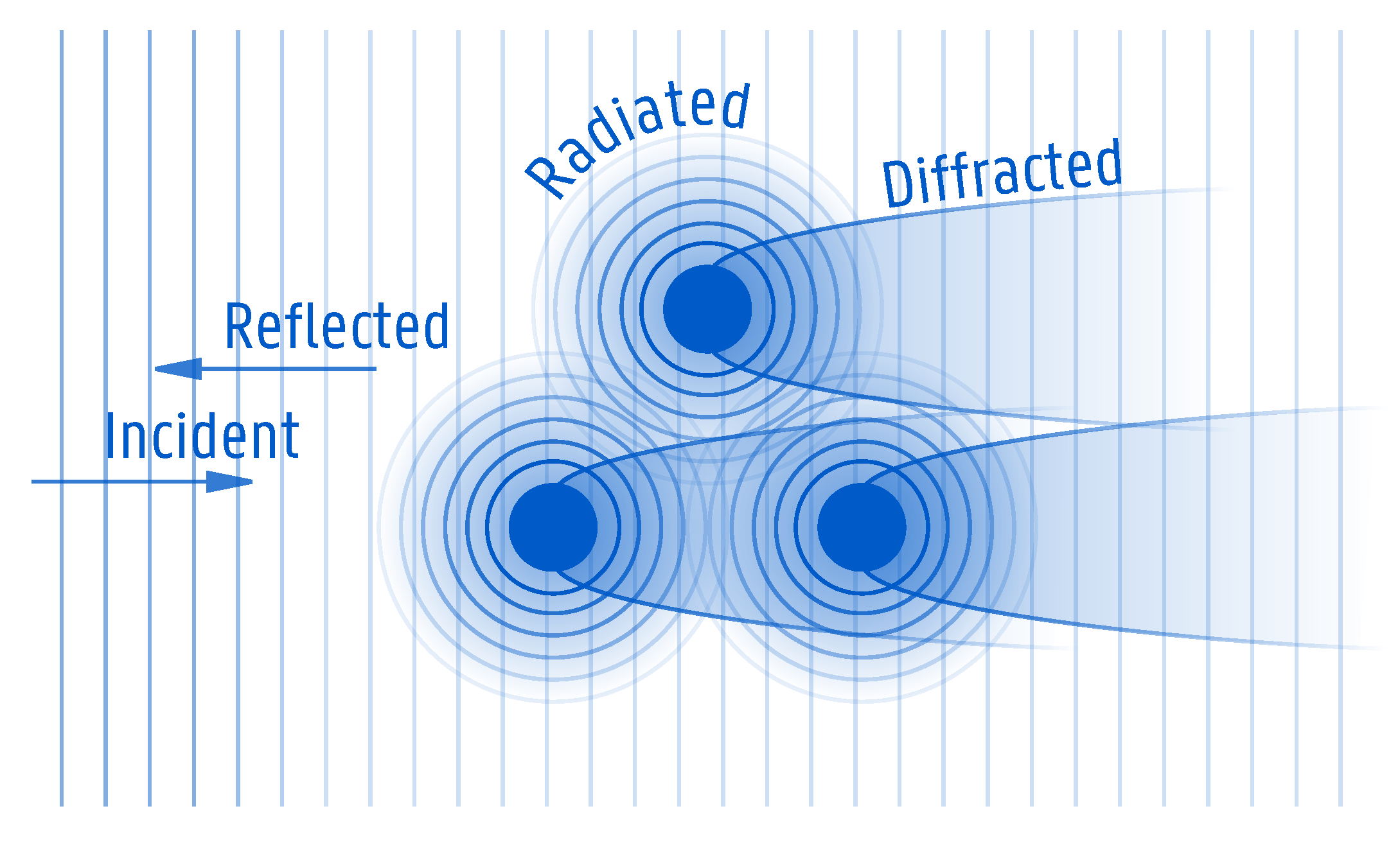
3]. Due to the interaction of the WECs with the incident waves, the following wave field physical processes, called “near-field effects”, take place:
Reflection: the incident wave encounters the WEC. A part of its energy is absorbed by the WEC; a part is transmitted past the WEC; and the remaining part is reflected, back to the open sea, with a smaller wave height and a different phase.
Diffraction: the waves undergo a change in direction as they pass around the WEC, as a result of the lateral yield of momentum flux, resulting in a concentric pattern, superimposed on the incident waves.
Radiation: as a response to the incident wave field, a WEC that is not fixed and has at least one degree of freedom will be put in motion, resulting in the creation of radiated waves.
The combination of the above physical phenomena results in a complex total wave field (see
Figure 1). At specific locations, the superposition of the waves leads to a higher energy content, called “hot spots”. In other locations, mostly in the lee of the WEC, there are wake effects, leading to a lower energy content. Consequently, it is important to have a good understanding of the location of hot spots and wakes in order to efficiently position a large number of WECs in an array layout. Moreover, this complex near-field wave field will propagate further outwards and have an effect on the far-field wave field, the so-called “far-field effects”. It has been shown that the maximum absorbed energy of point-absorbers is directly linked to the interaction of the radiated wave field with the incident wave field [
4]. Although this study mainly focuses on wave interactions with heaving point-absorber WECs, the described modeling methodology is applicable to any floating/fixed offshore structure/device.
The research presented in this paper focuses on the numerical modeling of wave-structure and wave-wave interactions within closely-spaced clusters of floating or fixed structures. Currently, there is no numerical model readily available to perform fast simulations of wave propagation in a large domain, over variable bathymetry, through closely-spaced structures; a choice has to be made between the use of accurate wave-structure interaction models with limited domain sizes and large domain wave propagation models, which lack the ability of accurately modeling complex wave fields. This research aims at overcoming these limitations by combining a wave-structure interaction solver and a wave propagation model to simulate wave propagation through closely-spaced clusters of floating or fixed structures, such as WECs or floating wind turbines.
Next, an overview of the numerical modeling of WEC arrays is given. Many different models exist and are based on various theoretical or applied approaches. Previous work [
5,
6,
7] has given an interesting overview of the different types of numerical models, and these studies concluded that all models have specific advantages and disadvantages and often result in making a decision between either computational speed or accuracy. In addition, the modeling can be performed in the frequency domain or the time domain. The first is typically known for fast computation times, but often leads to overestimation of absorbed power [
8]. The latter is necessary when combined wave-structure and wave-wave interaction are studied.
First, the wave-structure interaction models in the near-field are discussed. The most commonly-used models are the Boundary Element Method (BEM) potential flow solvers (e.g., Aquaplus [
9], ANSYS Aqwa [
10], WAMIT [
11], Nemoh [
12]). These calculate the frequency-dependent hydrodynamic properties of a single or multiple WEC devices. These tools allow one to study the near-field effects such as radiation and diffraction for a linear, regular incident wave over a flat sea bottom. Secondly, due to a better description of the related physics as presented in [
13], the use of codes resolving the Navier–Stokes equations (e.g., Computational Fluid Dynamics (CFD) models [
14,
15,
16,
17] and Smoothed Particle Hydrodynamics (SPH) [
18,
19,
20,
21]) for modeling WECs is growing nowadays. The governing equations are solved in the time domain; this means the physical variables do not have to be constant per frequency, but can vary in a non-linear manner over time (e.g., slack-lined mooring forces, non-linear PTO forces). The BEM and the Navier–Stokes-based solvers will be hereafter referred to as “wave-structure interaction solvers”.
The second group of numerical modeling tools focuses on wave propagation models, mainly applied to study far-field effects. Within these, a WEC or floating device is represented in a simplified way, e.g., by a porous structure that extracts a specific quantity of wave power from the incoming waves. The simulated WEC exhibits a specific amount of reflection, transmission and absorption of the incident waves. Firstly, there are the spectral propagation models. They consider a complete WEC array as a spatially-uniform energy sink [
22,
23,
24]. Often, these models are used to study the impact of a WEC farm on the coastal wave climate. The downsides of these type of models are the omission of the wave interactions in between WEC devices and the parametrized power absorption by the WEC. The most important drawback is the inaccurate representation of wave diffraction by the WECs. The whole WEC array is approximated as one giant structure absorbing a part of the incident wave energy. Secondly, there are time domain wave propagation models; a distinction can be made between wave propagation models based on mild-slope equations [
2,
25,
26,
27] and Boussinesq models [
28,
29,
30,
31].
All of the above-mentioned models suffer from a common problem: they cannot be used to model both near-field interactions and far-field effects, as recently reviewed in [
6,
32]. Models based on the Boundary Element Method (BEM) approach of potential flow theory or on the approach of Navier–Stokes equations suffer from a high computational cost, when simulating power absorption and the wave field alteration due to large WEC arrays. Simulation domains of non-constant water depth are prohibitive, which results also in restrictions on the number of the simulated WECs (typically less than 10 WECs). However, in order to investigate far-field effects, for example to study coastal impact, much larger computational domains are required.
On the other hand, the approach of wave propagation models enables simulation of these far-field effects. Large WEC arrays installed in large domains (several tens of kilometers) are modeled at a reasonable computational cost. As a result, the changes in wave field and the associated environmental impacts can be studied at the regional scale. However, the WECs are approximated up to now by using parametrized energy sinks and empirically tuned energy absorption coefficients. This method only partially addresses the underlying physics, which may lead to erroneous model conclusions. Moreover, when it comes to the modeling of oscillating WECs, the radiated wave field induced by the WEC’s motion is not considered in wave propagation models such as in [
33,
34,
35].
The present research focuses on introducing a generic coupling methodology, combining the near-field accuracy of wave-structure interaction models with time-efficient far-field wave propagation models. An application of this methodology has resulted in two “in-house” developed modeling tools; both of them combining the BEM wave-structure interaction model, Nemoh, with a fast wave propagation model. The first tool uses a depth-averaged mild-slope equation model called MILDwave [
27,
36], while the second one is a 3D, fully-non-linear potential flow solver called OceanWave3D [
29]. The latter model has the extra advantage of being able to calculate non-depth averaged wave kinematics. Near-field effects such as radiation and diffraction are calculated by the BEM solver, and the interaction with the incident waves and further propagation in the far-field over variable bathymetry are handled by the wave propagation model.
In
Section 2 of this paper, the coupling methodology is introduced. Next, the methodology is applied to a wave-structure interaction solver and two wave propagation models, to model both the near-field and far-field effects of wave propagation through a WEC array, as presented in
Section 3. In
Section 4, the results of the numerical models are compared through a large number of simulations, covering a wide spectrum of wave conditions and WEC array layouts. In addition, the OceanWave3D-Nemoh model is compared to an experimental dataset in
Section 4. The results of the present study are discussed in
Section 5 together with the concluding remarks.
2. Coupling Methodology
In this section, a numerical coupling methodology for predicting the wave field around devices or structures (single or in a park layout) is presented and is inspired by the work of [
26,
27], where an internal circular wave generation boundary around floating structures was applied to pass information from WAMIT [
11] to MILDwave and propagate the waves within the wave propagation domain. The present coupling methodology has been developed to combine:
the advantages of the approach of wave-structure interaction solvers, which accurately formulate and efficiently resolve the physical processes in wave energy absorption and floating structures;
and the benefits of the approach of wave propagation models, which efficiently resolve the propagation and transformation of waves over large distances, including bathymetric variability and wave transformation processes when approaching the coastline.
2.1. General Concept
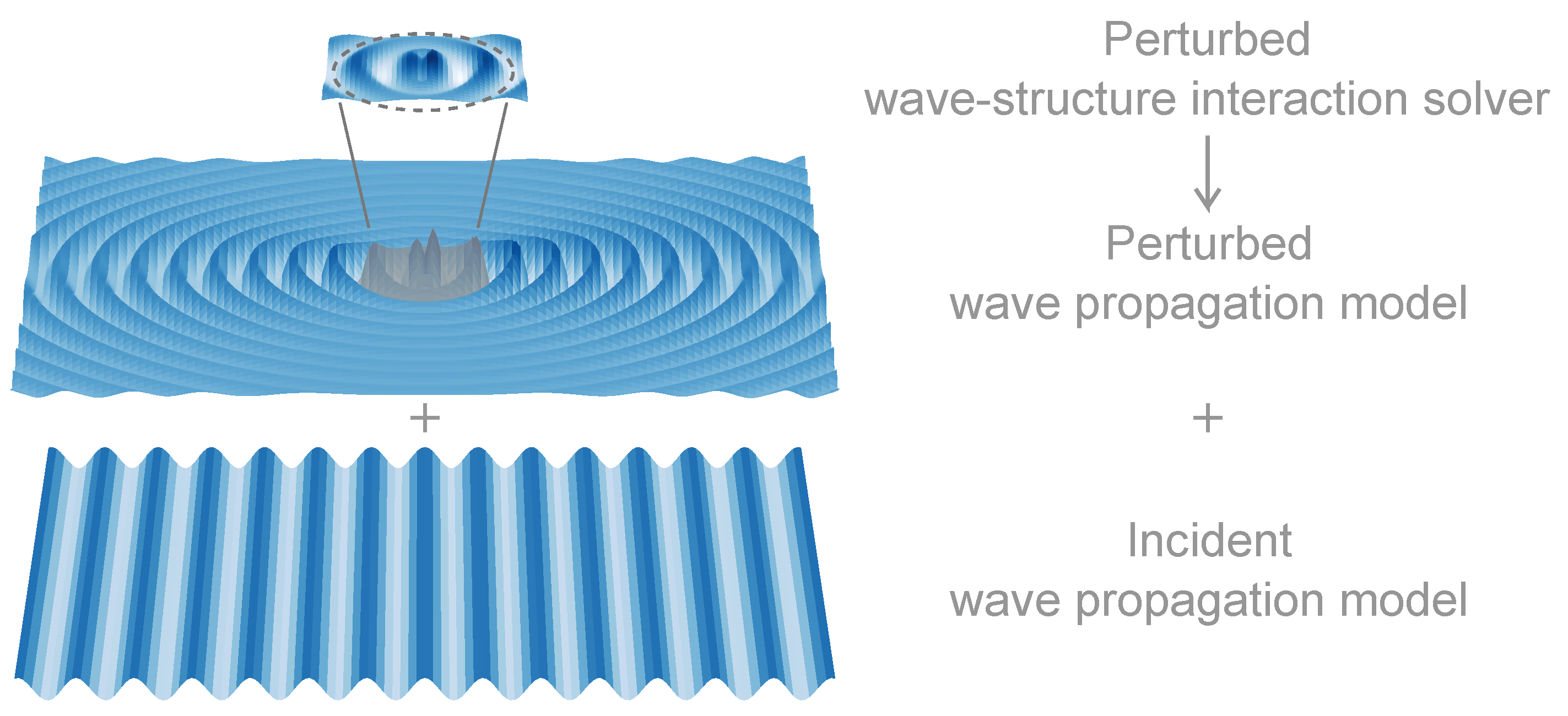
The goal of the coupling methodology is to predict the total wave field, by superposing the perturbed (reflected + diffracted + radiated) wave field and the incident wave field. For the perturbed waves, a frequency domain wave-structure interaction solver is used within a restricted zone around the floating or fixed devices. The propagation and transformation of the incident waves in a large domain is calculated by employing a wave propagation model. The coupling methodology is applicable to both floating and fixed offshore devices. However, in this paper, the focus is put on floating devices or structures, which is the most complex and computationally demanding case. The general concept is sketched in
Figure 2.
The main coupling mechanism is a superposition of two separate simulations: one for the perturbed wave field and another for the incident wave field. The perturbed wave field is a combination of the radiation and diffraction (including wave reflection) and is calculated during a first run in the frequency domain by the wave-structure interaction solver, within a restricted zone around the device/structure, indicated by the dashed circle in
Figure 2. Note that this zone can be used either around a single device/structure or around a cluster of devices/structures. Within the wave propagation model, the perturbed field is propagated outwards from the center of the domain. In a separate run, the incident waves are propagated over the entire domain in the wave propagation model. It is only after both runs have finished that the wave fields are superposed to result in the total wave field. This superposition principle is possible, since the linear wave theory is applicable.
2.2. Calculating the Perturbed Wave Field
The perturbed wave field is the superposition of the radiated and diffracted field and is calculated in two steps. First, a frequency domain simulation is performed in the wave-structure interaction domain with a flat bathymetry; here, we use a linear BEM solver, where the static and dynamic pressure are integrated over the floating body resulting in radiation and diffraction forces. These quantities depend on the body shape, the degrees of freedom, the wave period and the local water depth. Many different body shapes are possible, ranging from axisymmetric shapes to WEC devices, barges, ships and offshore platforms.
The wave-structure interaction calculation results in the complex, frequency-dependent radiated and diffracted wave fields (including the wave reflection), which are calculated on a rectangular grid. This grid is chosen smaller and finer than the wave propagation grid, which offers higher accuracy.
In the next step, the diffracted and radiated waves, as calculated in the previous step, are propagated in the wave propagation model with varying bathymetry. Specifically, they are imposed on a circular wave generation zone and are propagated towards the outside of the domain. At this point, it is to be noted that this internal wave propagation zone should not necessarily be circular and can be otherwise defined. In order to impose the perturbed wave field in the wave propagation model, it is necessary to transform both the radiated and diffracted wave field to the time domain within that coupling zone:
Within Equations (
1) and (
2),
is the radiated wave field in the time domain. This is a summation of the radiated wave field for each device/structure in the array.
is the diffracted wave field for the complete array.
A is the wave amplitude.
is the amplitude of the complex response amplitude operator for the corresponding device/structure
j, defined by Equation (
3) [
37], while
is the phase angle.
is the amplitude of the complex radiated wave field for device/structure
j and a specific frequency, coming directly from the wave-structure interaction model, while
is the phase angle.
is the amplitude of the diffracted wave field, while
is the phase angle. The parameters calculated with the BEM solver are indicated with bold font.
In Equation (
3),
is the complex wave excitation force,
the mass of device/structure
,
the added mass,
the hydrodynamic damping coefficient and
the hydrostatic stiffness. The effect of a linear Power Take-Off (PTO) system on the radiated wave field is taken into account by adding external mass
, damping
or spring coefficient
. The parameters calculated with the BEM solver are indicated with bold font.
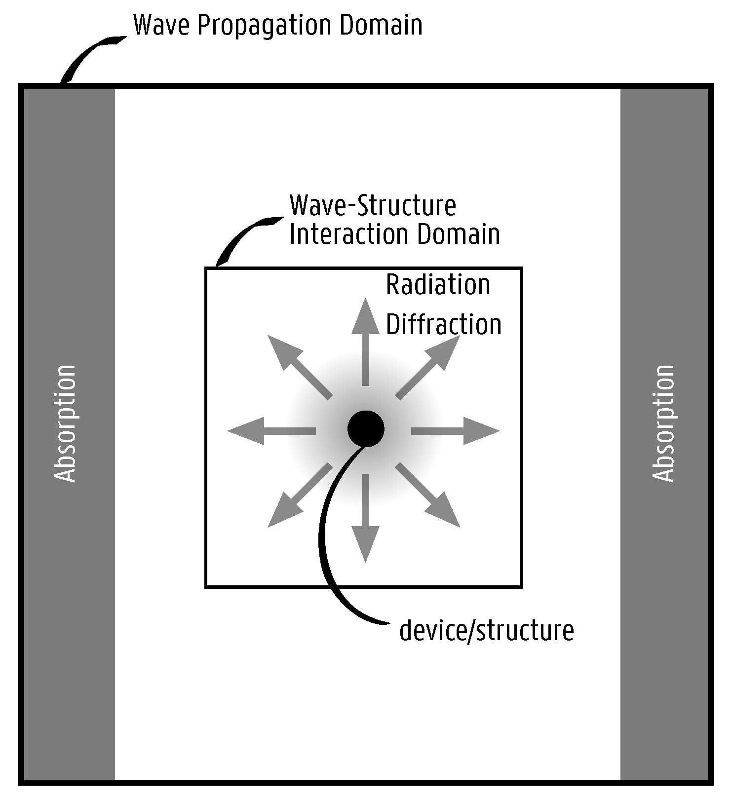
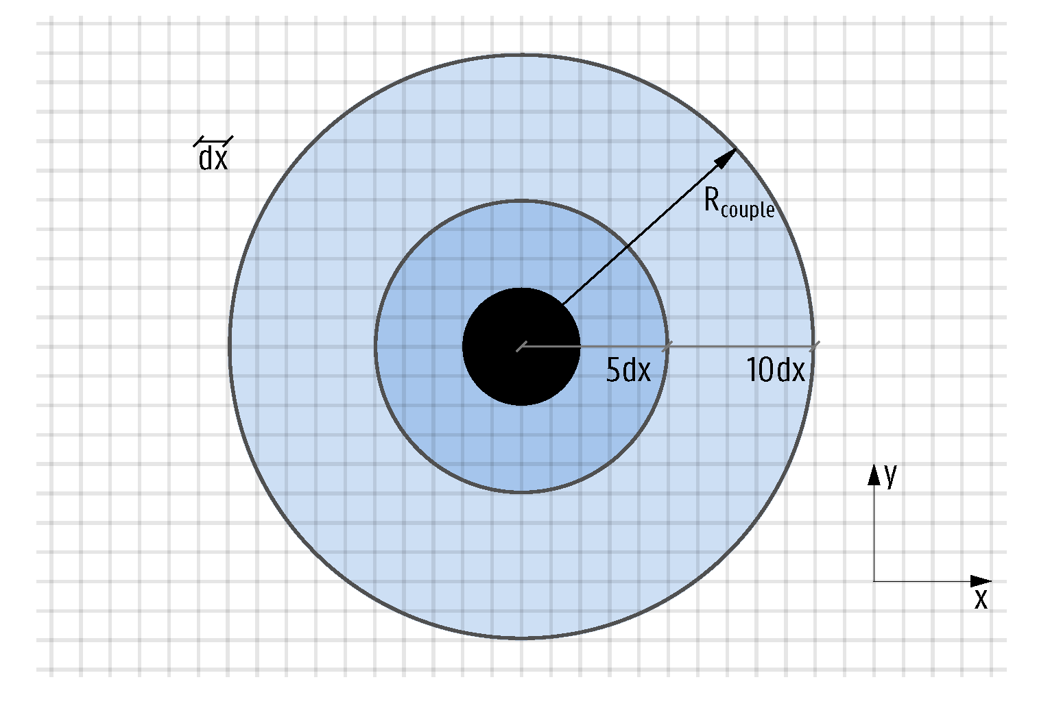
The perturbed (radiation + diffracted) wave field is propagated using the wave propagation model from within a circular zone around the device/structure (see
Figure 3). The circular area (light grey gradient) is a wave generation zone defined by a radius
, termed as the “coupling radius”. Within that circular zone, the surface elevation is imposed, so waves are forced to propagate away from the device/structure. At the interface between the wave generation zone and the wave propagation domain, the waves are released and propagate across the domain. From that point onwards, the governing wave propagation equations take over and take into account the (variable) bathymetry. At the left and right side of the wave propagation domain, wave absorbing boundary conditions such as relaxation zones or sponge layers are applied (dark grey zones).
2.3. Calculating the Incident Wave Field
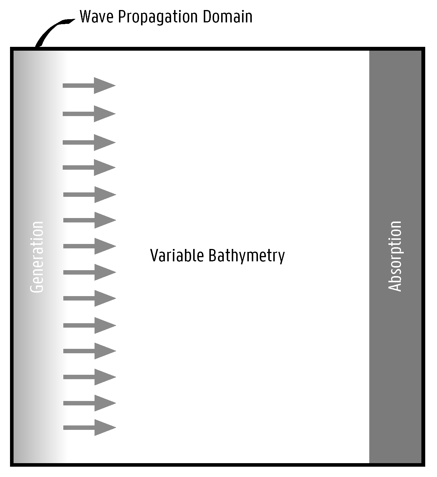
The incident wave field is directly calculated in the time domain within the wave propagation model. However, special attention is needed for the phase angle of the incident wave. It is important that at the center of the circular coupling zone, the phase angle is always equal to
. This is necessary since the perturbed wave field is coming from the frequency domain, where the phase is referenced with respect to the center of the device/structure. This phase matching is ensured by calculating the phase angle in the incident wave run, at the center of the coupling zone, and subtracting this value from the perturbed wave field phase angle. The numerical setup is illustrated in
Figure 4. The wave propagation models are able to simulate shoaling and refraction of incident waves over complex bathymetries. In the case of mild-slope equation models, the slopes need to remain within a gradient of
, while Boussinesq-type models and fully non-linear potential flow models can handle any type of bathymetry, however with a certain pre-processing and numerical instability cost [
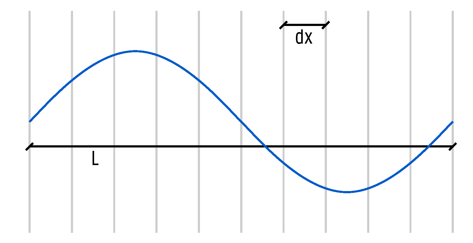
38]. At the left, boundary conditions of the generation of regular linear waves are applied:
In Equation (
4),
is the incident surface elevation,
A is the wave amplitude,
is the wave frequency (in rad/s),
k is the wave number and
is the wave direction. Waves propagate towards the right side, where the waves are absorbed by a relaxation boundary condition or a sponge layer. The top and bottom boundaries can be reflective (no-flux boundary condition) or absorbing, depending on the selected wave propagation model. When reflective boundaries are applied, it is advised to extend the wave propagation domain, perpendicular to the incident wave direction.
In the case of irregular incident waves, the superposition principle can be applied. A linear, irregular wave can be represented as a sum of a finite number of regular wave components, each with a characteristic wave height and wave period derived from the wave spectrum. In order to avoid local attenuation of the surface elevation
, each regular wave component should be shifted with a random phase angle
:
Modeling the wave propagation of irregular waves through a closely-spaced cluster of floating/fixed offshore devices requires performing multiple coupled simulations with regular waves, each shifted with a random phase angle, and finally superposing all individual regular wave fields.
3. Application of the Coupling Methodology
In this section, the coupling methodology, described in
Section 2, will be demonstrated for predicting WEC array effects. Moreover, it will be demonstrated for two different wave propagation models. First, the employed wave-structure interaction solver is discussed, followed by the two wave propagation models. Next, the results obtained by the coupling methodology implemented in these two wave propagation models will be compared to each other and to experimental data.
3.1. Wave-Structure Interaction Model
The wave-structure interaction solver used in this research is the open-source software package Nemoh, developed at Ecole Centrale de Nantes [
12]. The current Version v2.03 is based on linear potential flow theory and thus makes the following assumptions:
The fluid is inviscid;
The fluid is incompressible ;
The flow is irrotational;
The wave amplitude is small w.r.t. the wavelength;
The amplitude of the body motion is small w.r.t. its dimension;
The sea bottom is flat;
The flow is described by a velocity potential
, as a function of time and space. The flow field
is expressed as the gradient of the velocity potential:
Combining Equation (
6) with Assumption 2 leads to the well-known Laplace equation:
This equation is valid in the entire fluid domain, denoted
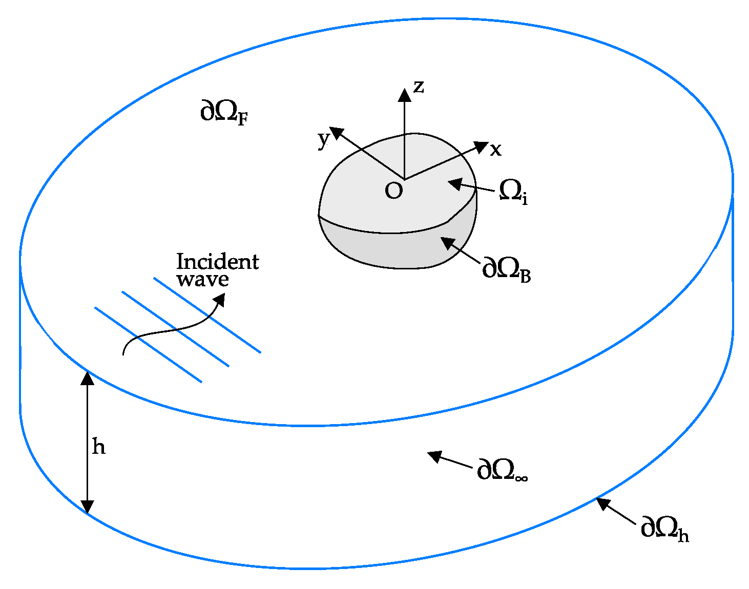
. The whole velocity potential problem becomes then a linear Boundary Value Problem (BVP), visually represented in
Figure 5. The boundary conditions are given in the set of Equation (
8).
Here, is a given point in the fluid domain, is a scalar function, is the wave number solution of the dispersion relation and is the incident wave potential at infinity. The boundary conditions are expressed over the different boundary surfaces, where the indices stand for:
This 3D problem can be transformed into the 2D problem of a source distribution on the body surface using Green’s second identity and the appropriate Green function [
9,
39]. The mathematical problem is then discretized using a constant panel method, leading to a linear matrix problem whose coefficients are the influence coefficients. The BVP is numerically solved in the frequency domain; leading to the full flow field underneath the body. From the flow field, several other quantities are calculated:
The hydrodynamic coefficients: added mass and hydrodynamic damping ;
The pressure field p on the body surface and the Froude–Krylov forces ;
Far-field diffracted and radiated velocity potential in the form of Kochin functions;
Near-field diffracted and radiated surface elevation and ;
These quantities are necessary for the coupling with each of the wave propagation models, which are discussed in the next section.
3.2. Wave Propagation Models
The second part of the coupling methodology is the wave propagation model. This model propagates the incident waves and predicts their interaction with the diffracted and radiated waves as predicted by Nemoh. For this, two separate software packages are applied: MILDwave, a 2D model based on mild-slope equations, and OceanWave3D, a 3D model based on fully non-linear potential flow equations. We will denote the coupled models as the MILDwave-Nemoh model and the OceanWave3D-Nemoh model, respectively.
3.2.1. MILDwave
In simulating the far-field effects, the wave propagation model MILDwave is employed [
27,
36]. MILDwave, developed at the Coastal Engineering Research Group of Ghent University, Belgium, is a phase-resolving model based on the depth-integrated mild-slope Equations (
9) and (
10) by Radder and Dingemans [
40]. This particular model has been used also in modeling WEC arrays in a number of recent studies [
26,
27,
41,
42,
43,
44,
45]. The mild-slope Equations (
9) and (
10) are solved using a finite difference scheme that consists of a two-step space-centered, time-staggered computational grid, as detailed in [
46].
Here, and are, respectively, the surface elevation and the velocity potential at the free water surface, g is the gravitational acceleration, C is the phase velocity and the group velocity for a wave with wave number k and angular frequency .
3.2.2. OceanWave3D
The second applied wave propagation model is called OceanWave3D. The software is open-source and applies a fully-non-linear potential flow solver [
29,
47]. It is aimed at closing the performance gap between traditional Boussinesq-type models and volume-based solvers and enables fast (near) real-time hydrodynamics calculations. The fully-non-linear potential flow problem for waves on a fluid of variable depth is applied to find the free surface elevations on a 3D grid, with vertical sigma layers. This allows for the prediction of velocity profiles, in contrast to MILDwave, which only supports depth-averaged velocities. The evolution of the free surface is governed by the kinematic and
dynamic boundary conditions:
These are expressed as a function of the free surface quantities and . The problem is discretized using a method of lines approach, and for the time-integration of the free-surface conditions, a classical explicit four-stage, fourth-order Runge–Kutta scheme is employed. Spatial derivatives are replaced by the discrete counterparts using the high-order finite difference method, and non-linear terms are treated by direct product approximations at the collocation points. At the structural boundaries of the domain, i.e., at the bottom and wall sides, Neumann conditions are imposed. When applying the coupling method to OceanWave3D, the non-linear effects are omitted. Consequently, the linear superposition method can be applied and the total transformed wave field can be created by summation of the independent surface elevations and potentials.
3.3. Experimental Dataset
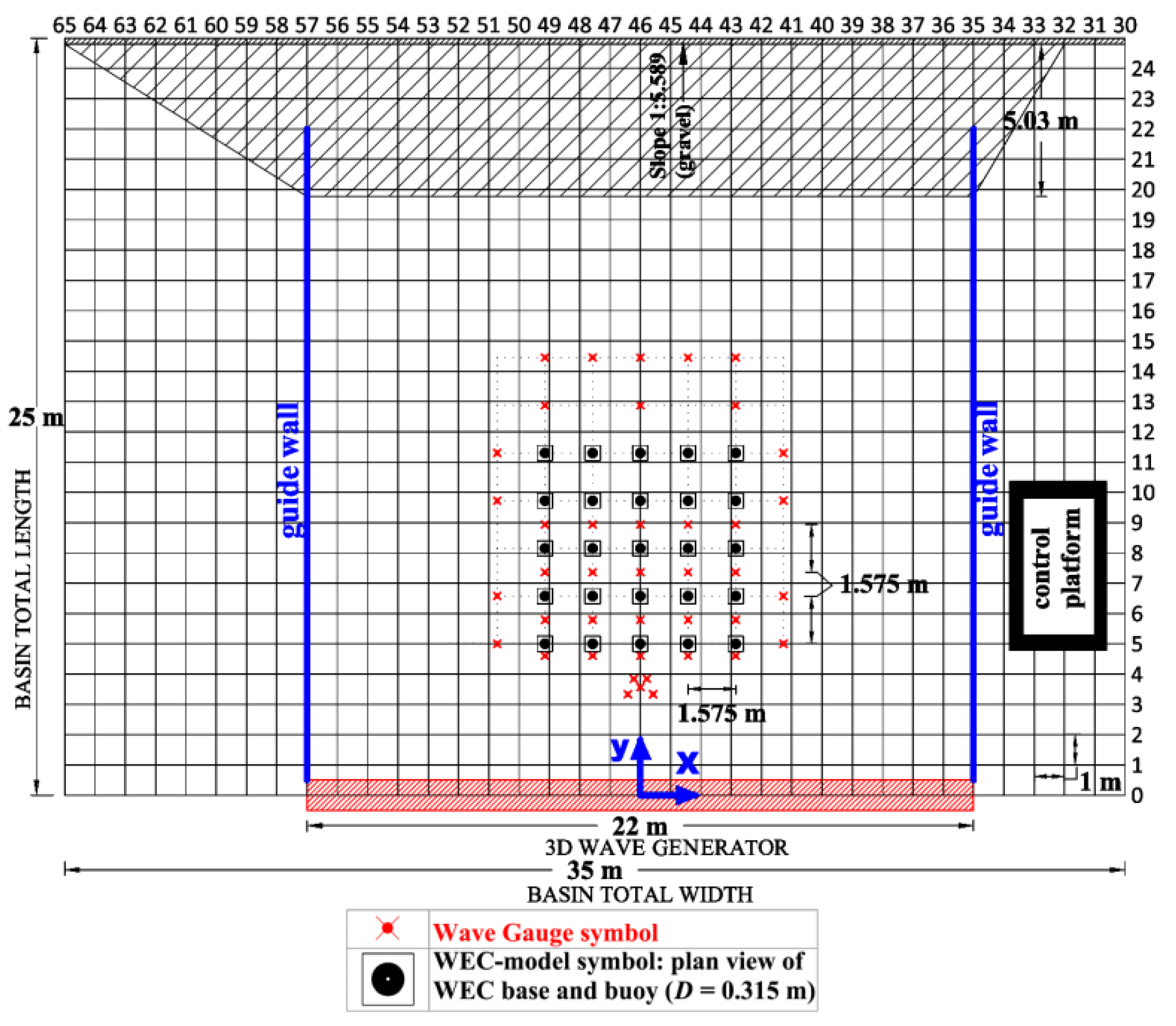
In 2013, as part of the WECwakes research project funded by the EU FP7 HYDRALAB IV program, experiments have been conducted in the Shallow Water Wave Basin of the Danish Hydraulic Institute (DHI) in Hørsholm, Denmark [
3]. A large number of tests was performed on large arrays of point absorber-type WECs (up to 25 units, see
Figure 6). The research performed within the WECwakes project focuses on generic heaving WECs, intended for validation purposes of numerical models.
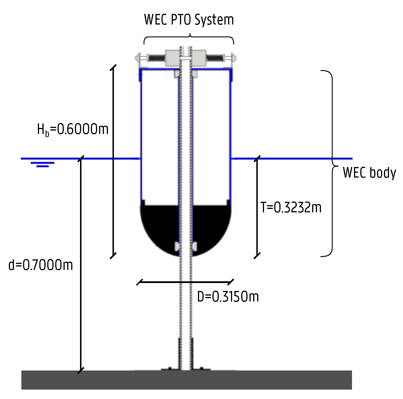
A range of WEC array geometric configurations and wave conditions have been tested. Each WEC unit is composed of a buoy, designed to heave along a vertical shaft only, and can thus be modeled as a single degree of freedom system (see
Figure 7). The WEC consists of a cylindrical body and a spherical bottom. The diameter is 0.3150 m, while the draft is 0.3232 m. The water depth is fixed at 0.7000 m. Energy absorption through the WECs’ PTO system, is modeled by realizing energy dissipation through friction-based damping of the WECs’ heave motion. Wave gauges are used to measure the wave field within and around the arrays. Displacement meters are mounted on each WEC unit for the measurement of the heave displacement. The wave induced surge force is measured on five WECs along the central line of the array.
The experimental setup of 25 individual WEC units in an array layout, placed in the large wave tank, is at present the largest setup of its kind, studying the important impacts on power absorption and wave conditions of WEC array effects. Most importantly, the WECwakes database is comprehensive and is applicable not only to WEC arrays, but also to floating structures/platforms, stationary cylinders under wave action, etc., for understanding of, e.g., wave impact on the cylinders and wave field modifications around them. The WECwakes database is accessible to the research community as specified under the HYDRALAB rules.
3.4. Test Program
3.4.1. Comparison between Wave Propagation Models Using the Coupling Methodology
The first objective of this research is to compare the results obtained by the application of the introduced coupling methodology to both wave propagation models. For this reason, a test program based on long-crested regular and irregular waves is set up, as presented in
Table 1. The WEC-WEC distance
is fixed at
with
D the diameter of the WEC. A cylindrical device is chosen with
m and a draft of
m. The following characteristics are varied during the tests:
Wave type: regular (REG) and irregular waves (IRR)
Water depth d: deep and transitional water
Number of WECs: ranging from one to five
Array geometrical layout: several configurations
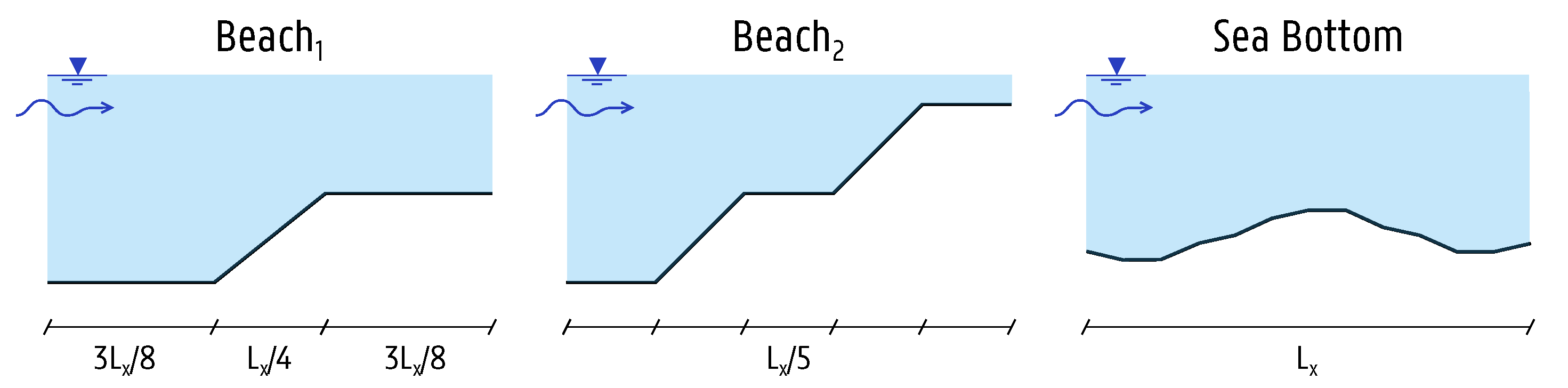
Bathymetry: fixed bottom; two beach profiles (Beach1, Beach2); one sea bottom
Tests 3 to 10 are performed with multiple WECs. It is important to mention that the coupling methodology is applied by coupling the complete array of WECs, instead of coupling each WEC individually. Tests 7 to 9 and 10 are performed with varying bathymetry. Test 7 refers to wave propagation over a gradual beach slope (Beach
1) with a gradient of
going from 50 m depth to 25 m over a length of 300 m. The bathymetry of Test 8 (Beach
2) consists of two consecutive beach slopes with a gradient of around
with water depths from 50 m to 25 m to 1 m. Finally, Tests 9 and 10 are based on a sea bottom bathymetry with an average depth of 37 m. All bottom profiles are illustrated in
Figure 8.
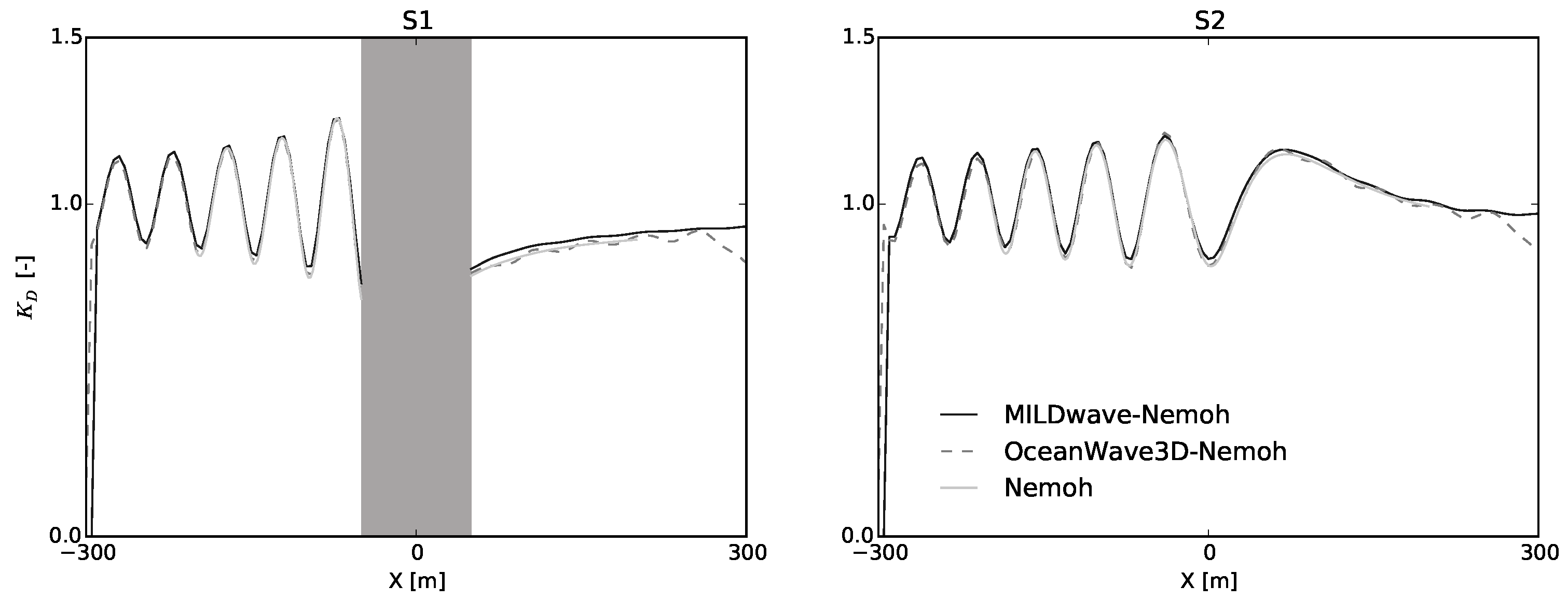
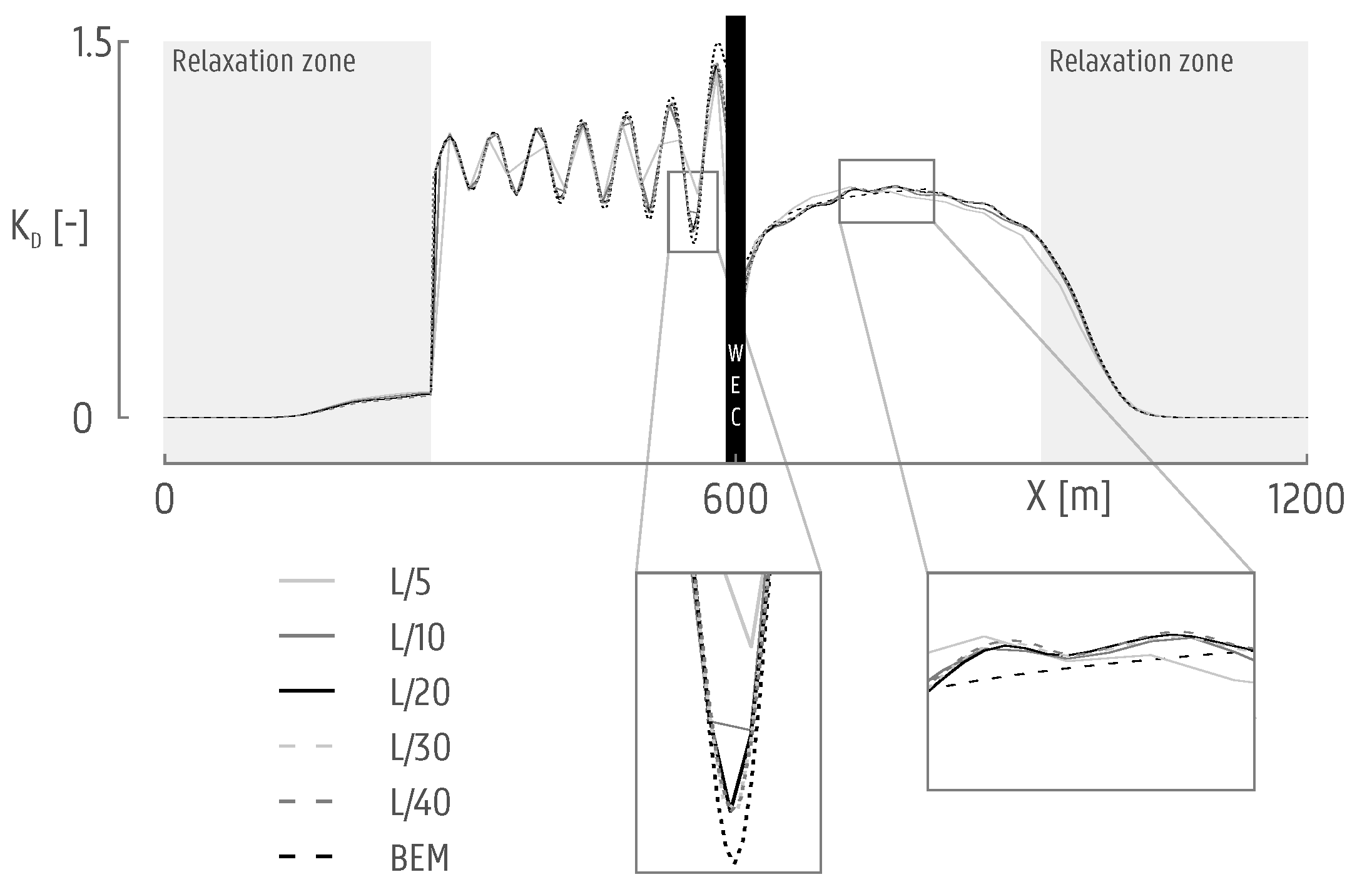
The accuracy of the results will be assessed by calculating the
value, over a specific time window
, as defined in Equation (
13). It is the ratio of the numerically-calculated disturbed wave height
to the incident wave height
. The surface elevation
is squared and summed up over all
n time steps within the time window
. It is multiplied with the relative time step
and a factor of eight. From this value, the square root is taken and finally divided by the incident wave height
(for regular waves) or significant wave height
(for irregular waves).
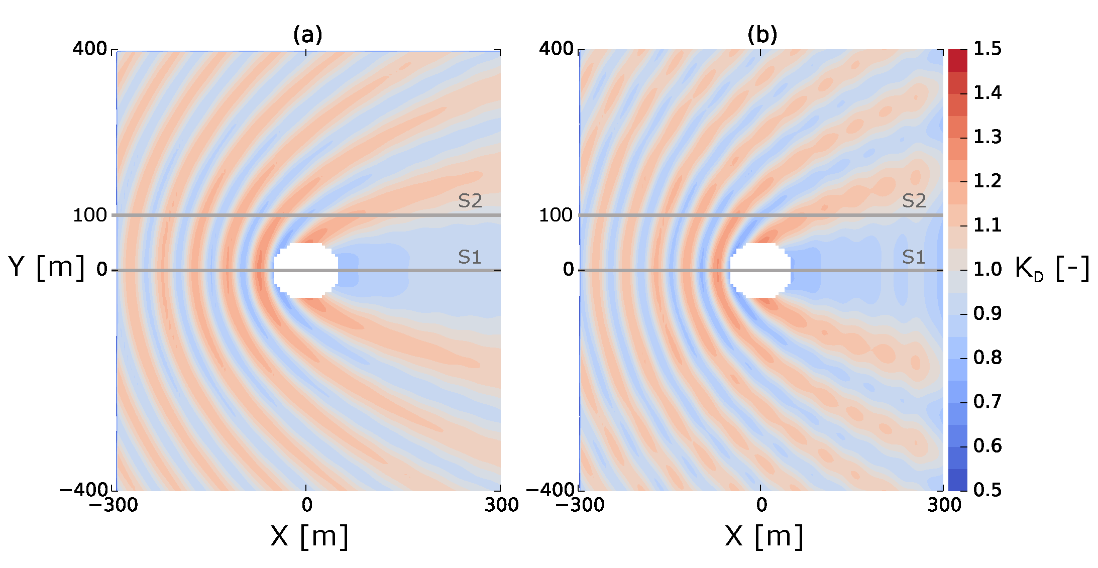
The value summarizes the wave interactions during the entire simulation duration in one value per grid cell. When , it indicates a local increase of wave height or “hot spot”, while a value indicates a local decrease of wave height or “wake”.
Within the comparison study, results from both wave propagation models are compared with each other. Additionally, the results are compared to a pure BEM solution where possible (regular waves with constant water depth). The accuracy of the models is estimated based on the following outputs:
Contour plots of the values throughout the entire domain
Line cross-sections of the values along the wave direction
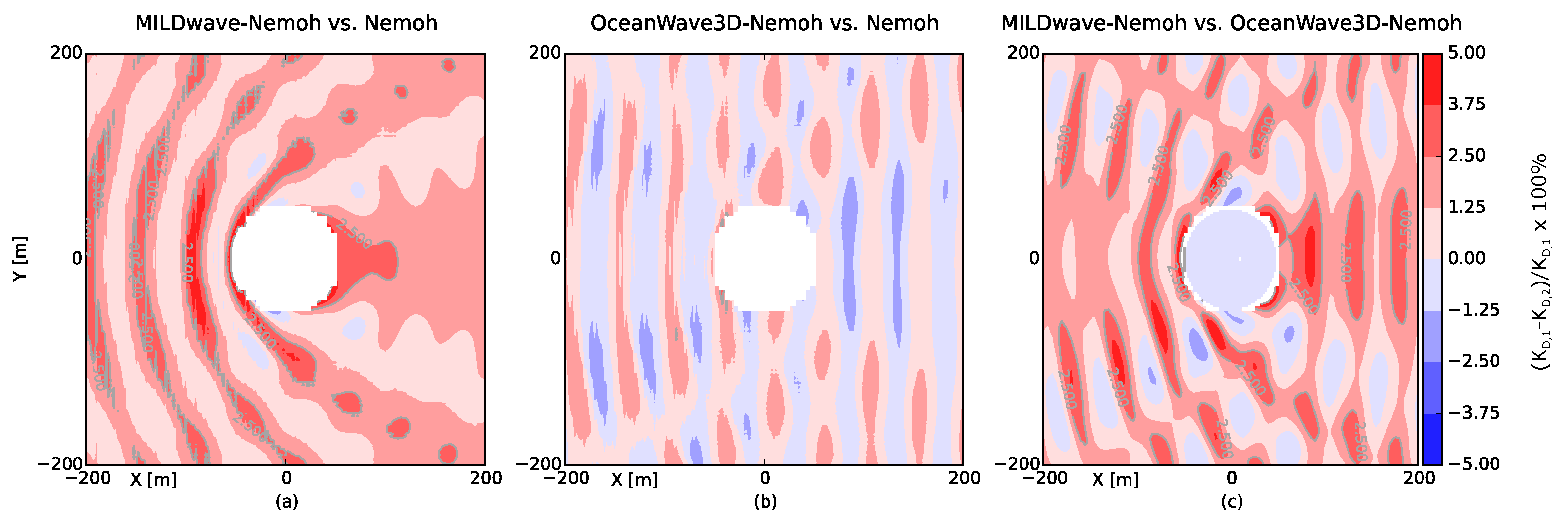
Contour plots of the relative differences between the results obtained by the wave propagation models
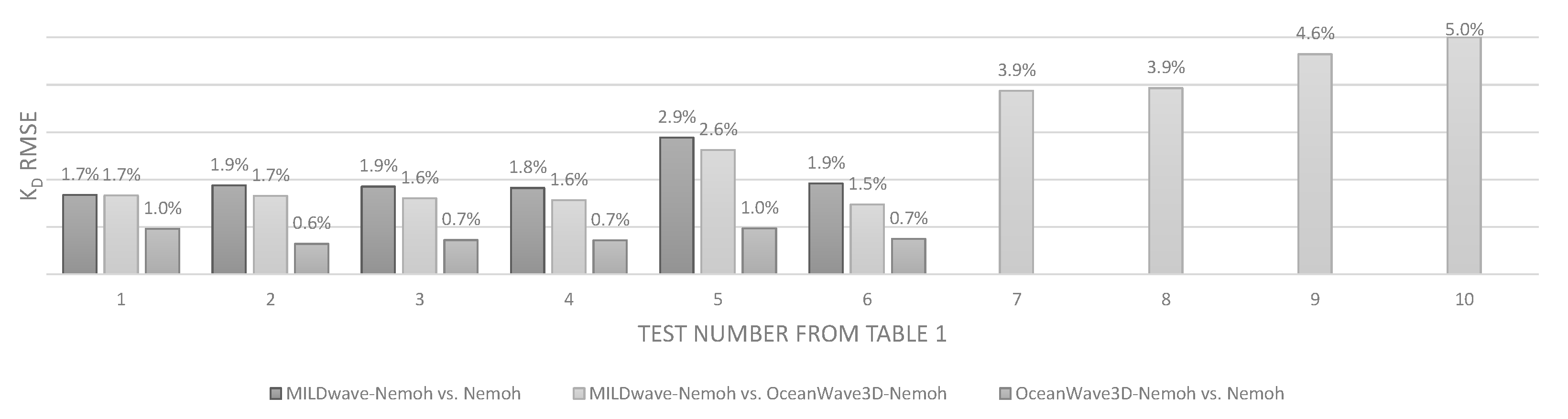
Calculation of relative error values
3.4.2. Comparison to Experimental Data
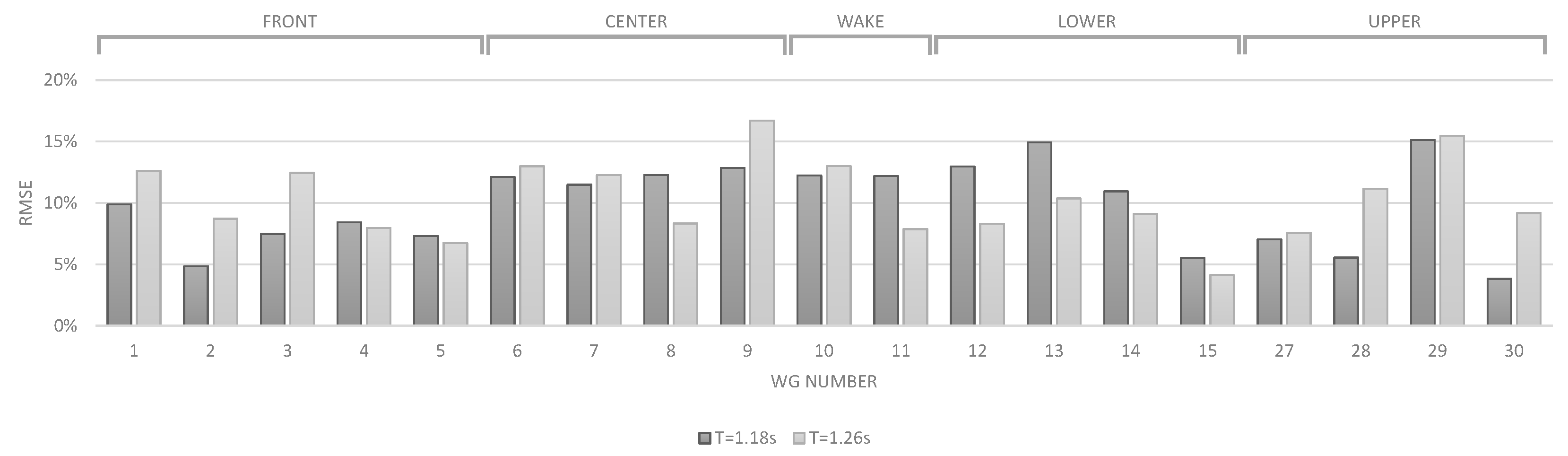
The WECwakes experiments consisted of 591 tests in total. Out of these tests, one geometrical array configuration is selected for the comparison with the results of the coupling methodology. There are two sets of regular incident wave conditions with wave height
m and wave period
T, either
s (close to the resonance period
of the device) or
s. These wave conditions, combined with a constant water depth of
m, result in non-linear Stokes second order waves. Although the numerical model is only valid for linear waves, the incident waves are only weakly non-linear. The wave propagation model OceanWave3D will be ran in non-linear mode, in contrast to what was advised in
Section 3.2.2, to ensure maximum accuracy of incident waves. Superposing the weakly non-linear incident and perturbed waves will lead to an error smaller than
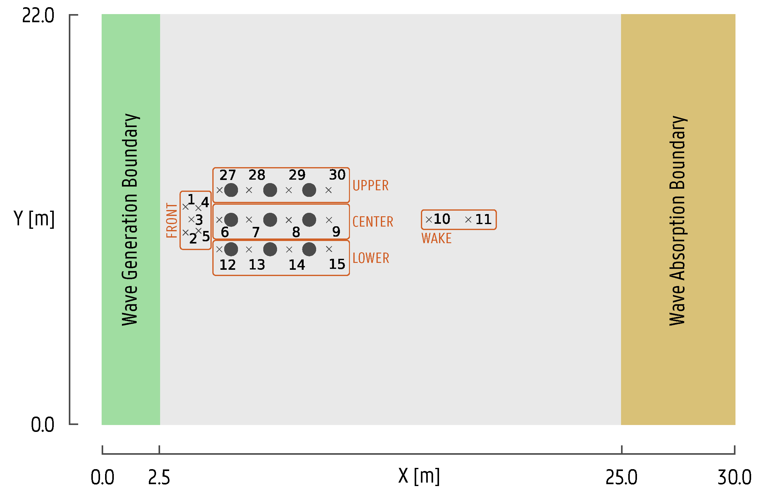
on the wave trough in comparison to linear wave theory, justifying the application of the superposition principle. The comparison is performed for a configuration of nine WEC units, arranged in a 3 × 3 layout (see
Figure 9). The WEC units have an equal spacing of five WEC diameters
m.
The DHI wave basin has a wave generation width of 22 m, while the waves propagate over a length of 25 m. Side walls are installed in the basin to guide the incident waves and reflect the perturbed waves. This is mainly done to simplify the comparison to numerical models, where it is difficult to absorb waves from different directions.
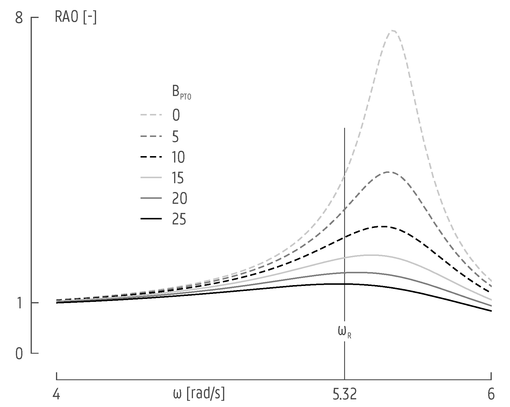
Each WEC unit is equipped with a friction-based PTO system. The effect of this PTO is included in the simulations by adding an external numerical damping term
to the RAO, as previously demonstrated in Equation (
3). In order to identify the correct value for this added damping, the RAO is calculated for several values of
. When the peak of the RAO curve is located exactly on the natural frequency
rad/s, the external damping is considered correct. As illustrated in
Figure 10, the correct value of
lies between 20 and 25 kg/s. Further iterations lead to a value of
kg/s.
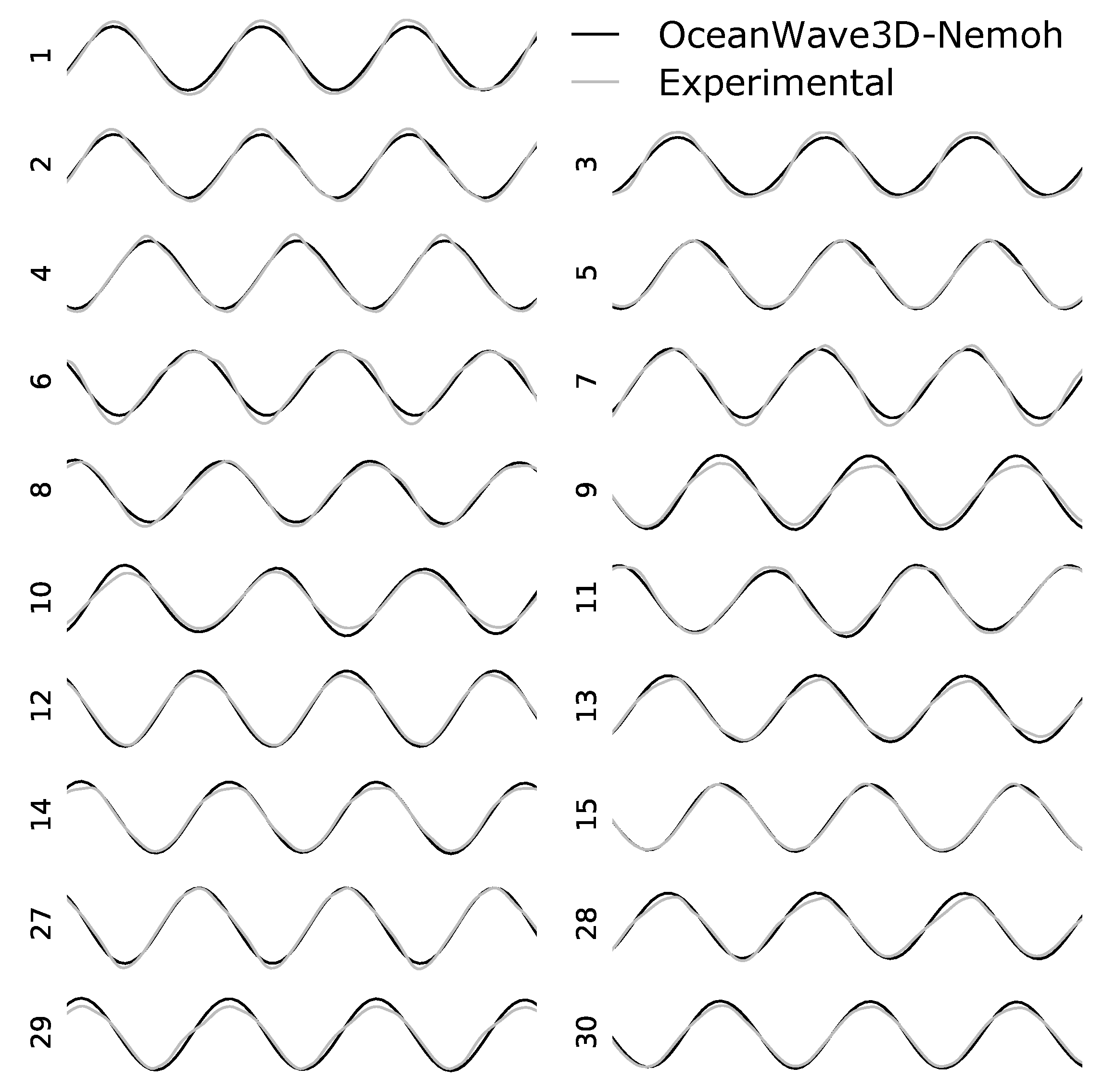
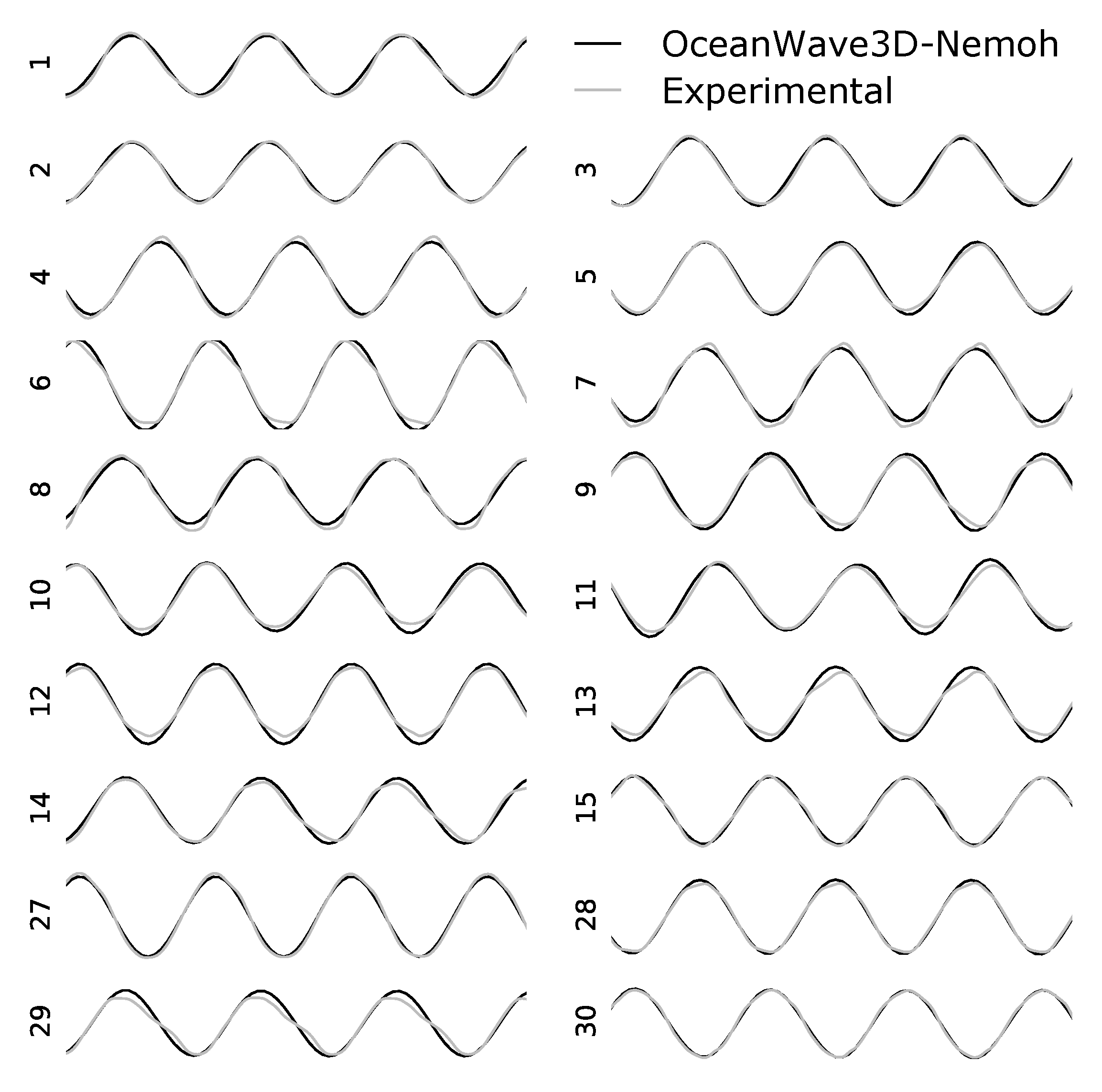
The comparison of the results is based on the surface elevation, registered by 19 resistive wave gauges, distributed over the domain as illustrated in
Figure 9. For each wave gauge, the surface elevation is compared to the signal obtained by the numerical model. The location of the wave gauges is not perfectly aligned with the computational grid, so results are interpolated. The accuracy of the numerical model is quantified by calculating the normalized RMSE between the surface elevation of the numerical model and the experimental data:
Additionally, the domain is shown in
Figure 9, measuring 30 m long and 22 m wide, with a 2.5 m-long wave generation zone and a 5 m-long wave absorption boundary. The grid size is set to
dx = 0.1 m, which corresponds to the suggested value of
, as explained in
Section 4.1.1. The time step is set to
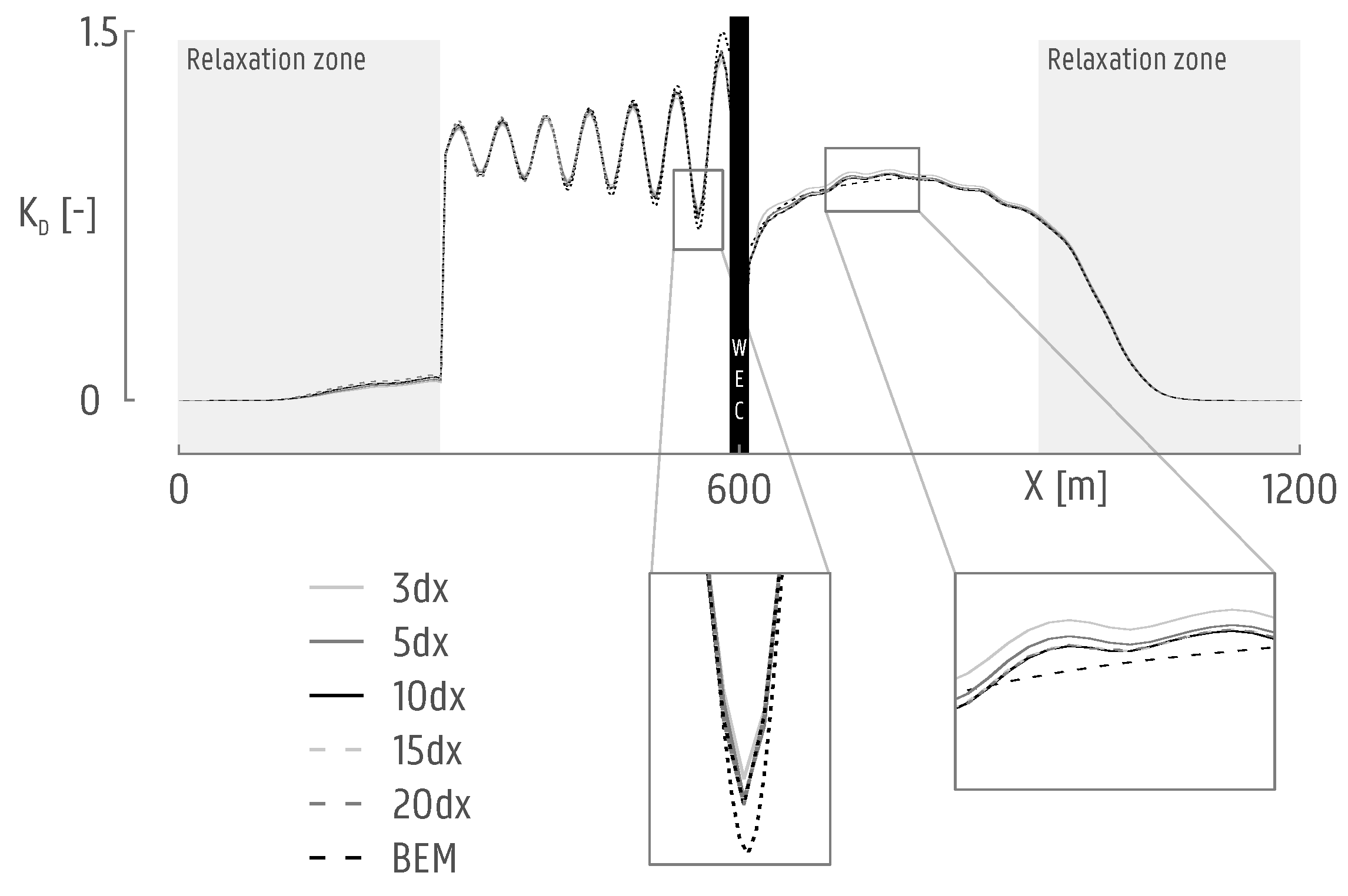
dt = 0.05 s, and the coupling radius is
Rc = 10,
dx = 1 m (see
Section 4.1.2).
5. Conclusions
In this paper, a generic coupling methodology was introduced to perform numerical modeling of (closely-spaced) offshore floating or fixed structures. By combining the accurate near-field wave-structure interaction solver with fast far-field wave propagation models, it is possible to model regular and irregular waves propagating through offshore device clusters over a variable bathymetry. This was demonstrated by employing two different wave propagation models, MILDwave and OceanWave3D, to model wave propagation through floating wave energy converter arrays. The numerical comparison proved that both MILDwave-Nemoh and OceanWave3D-Nemoh are capable of providing accurate surface elevations for a range of different test cases. In general, it is advised to apply MILDwave-Nemoh, since it calculates reasonably faster. However, OceanWave3D-Nemoh can be applied for bathymetries with steep slopes, for the calculation of non-depth averaged 3D simulations and weakly non-linear simulations.
The introduced coupling methodology has limitations, as well. Firstly, since the methodology uses the superposition principle for obtaining a total wave field, only linear waves conditions lead to correct results. However, applying the methodology to weakly non-linear wave conditions only introduces a small error, as demonstrated in
Section 4.3. Secondly, within the coupling zone, the solution is coming solely from the wave-structure interaction solver. It is thus necessary to have a flat bottom within that zone. Thirdly, typical BEM wave-structure interaction solvers are limited to a maximum number of fixed or floating bodies (e.g., Nemoh allows up to 25 bodies). However, in practice, they are enough for typical device farm applications. This limitation can be solved by applying a different type of wave-structure interaction solver. Fourthly, the coupling methodology does not allow direct simulation of irregular waves. Only a summation of several regular waves can be applied, which leads to an increase of the computational time.
In conclusion, despite some limitations, the coupling methodology has proven to be a valuable tool that is applicable in the following fields:
Far-field simulations of fixed/floating offshore devices, such as assessment of coastal impact, with significant higher accuracy than previously applied spectral methods;
Generic wave-wave and wave-structure interactions;
Assessing energy production of large WEC arrays;
Assessing wave propagation through large floating or fixed structure arrays, e.g., floating wind farms;
Optimization of floating or fixed structure array layout, based on the local wave climate and bathymetry.

 ,
, 


