Applications of Hybrid EMD with PSO and GA for an SVR-Based Load Forecasting Model


1
College of Mathematics & Information Science, Ping Ding Shan University, Pingdingshan 467000, China
2
School of Education Intelligent Technology, Jiangsu Normal University, 101 Shanghai Rd., Tongshan District, Xuzhou 221116, China
*
Author to whom correspondence should be addressed.
Energies 2017, 10(11), 1713; https://doi.org/10.3390/en10111713
Submission received: 30 September 2017
/
Revised: 19 October 2017
/
Accepted: 21 October 2017
/
Published: 26 October 2017
(This article belongs to the Special Issue Hybrid Advanced Optimization Methods with Evolutionary Computation Techniques in Energy Forecasting)
Abstract
:Providing accurate load forecasting plays an important role for effective management operations of a power utility. When considering the superiority of support vector regression (SVR) in terms of non-linear optimization, this paper proposes a novel SVR-based load forecasting model, namely EMD-PSO-GA-SVR, by hybridizing the empirical mode decomposition (EMD) with two evolutionary algorithms, i.e., particle swarm optimization (PSO) and the genetic algorithm (GA). The EMD approach is applied to decompose the load data pattern into sequent elements, with higher and lower frequencies. The PSO, with global optimizing ability, is employed to determine the three parameters of a SVR model with higher frequencies. On the contrary, for lower frequencies, the GA, which is based on evolutionary rules of selection and crossover, is used to select suitable values of the three parameters. Finally, the load data collected from the New York Independent System Operator (NYISO) in the United States of America (USA) and the New South Wales (NSW) in the Australian electricity market are used to construct the proposed model and to compare the performances among different competitive forecasting models. The experimental results demonstrate the superiority of the proposed model that it can provide more accurate forecasting results and the interpretability than others.
1. Introduction
Due to the difficult-reserved property of electricity, providing accurate load forecasting plays an important role for the effective management operations of a power utility, such as unit commitment, short-term maintenance, network power flow dispatched optimization, and security strategies. On the other hand, inaccurate load forecasting will increase operating costs: over forecasted loads lead to unnecessary reserved costs and an excess supply in the international energy networks; under forecasted loads result in high expenditures in the peaking unit. Therefore, it is essential that every utility can forecast its demands accurately.
There are lots of approaches, methodologies, and models proposed to improve forecasting accuracy in the literature recently. For example, Li et al. [1] propose a computationally efficient approach to forecast the quantiles of electricity load in the National Electricity Market of Australia. Arora and Taylor [2] present a case study on short-term load forecasting in France, by incorporating a rule-based methodology to generate forecasts for normal and special days, and by a seasonal autoregressive moving average (SARMA) model to deal with the intraday, intraweek, and intrayear seasonality in load. Takeda et al. [3] propose a novel framework for electricity load forecasting by combining the Kalman filter technique with multiple regression methods; Zhao and Guo [4] propose a hybrid optimized grey model (Rolling-ALO-GM (1,1)) to improve the accurate level of annual load forecasting. For those applications of neural networks in load forecasting, the authors of references [5,6,7,8,9] have proposed several useful short-term load forecasting models. For these applications of hybridizing popular methods with evolutionary algorithms, the authors of references [10,11,12,13,14] have demonstrated that the forecasting performance improvements can be made successfully. These proposed methods could receive obvious forecasting performance improvements in terms of accurate level in some cases, however, the issue of modeling with good interpretability should also be taken into account, as mentioned in [15]. Furthermore, these proposed models are almost embedded with strong intra-dependency association to experts’ experiences, as well as, they often could not guarantee to receive satisfied accurate forecasting results. Therefore, it is essential to propose some kind of combined model, which hybridizes popular methods with advanced evolutionary algorithms, also combining expert systems and other techniques, to simultaneously receive high accuracy forecasting performances and interpretability.
Due to advanced higher dimensional mapping ability of kernel functions, support vector regression (SVR) is drastically applied to deal with the forecasting problem, which is with small but high dimensional data size. SVR has been an empirically popular model to provide satisfied performances in many forecasting problems [16,17,18]. As it is known that the biggest disadvantage of a SVR model is the premature problem, i.e., suffering from local minimum when evolutionary algorithms are used to determine its parameters. In addition, its robustness also could not receive a satisfied stable level. To look for effective novel algorithms or hybrid algorithms to avoid trapping into local minimum, and to simultaneously receive satisfied robustness is still the very hot point in the SVR modeling research fields [19]. In the meanwhile, to improve the forecasting accurate level, it is essential to extract the original data set with nonlinear or nonstationary components [20] and transfer them into single and conspicuous ones. The empirical mode decomposition (EMD) is dedicated to provide extracted components to demonstrate high accurate clustering performances, and it has also received lots of attention in relevant applications fields, such as communication, economics, engineering, and so on [21,22,23]. As aforementioned, the EMD could be applied to decompose the data set into some high frequency detailed parts and the low frequent approximate part. Therefore, it is easy to reduce the interactions among those singular points, thereby increasing the efficiency of the kernel function. It becomes a useful technique to help the kernel function to deal well with the tendencies of the data set, including the medium trends and the long term trends. For determining the values of the parameters in a SVR model well, it attracts lots of relevant researches during two past decades. The most effective approach is to employ evolutionary algorithms, such as GA [24,25], PSO [26,27], and so on [28,29]. Based on the authors’ empirical experiences in applying the evolutionary algorithms, PSO is more suitable for solving real problems (with more details of data set), it is simple to be implemented, its shortcoming is trapped in the local optimum. For GA, it is more suitable for solving discrete problems (data set reveals stability), however one of its drawbacks is Hamming cliffs. In this paper, the data set will be divided into two parts by EMD (i.e., higher frequent detail parts and the lower frequent part), the higher frequency part is the so-called shock data which demonstrates the details of the data set, thus, SVR’s parameters for this part are suitable to be determined by PSO due to its suitable for solving real problems. The lower frequency part is the so-called contour trend data which reveals its stability, thus, SVR’s parameters for this part could be selected by GA due to its suitable for solving discrete problems.
Therefore, in this paper, the mentioned two parts divided by EMD are conducted by SVR-PSO and SVR-GA, respectively; eventually the improved forecasting performances of proposed model (namely EMD-PSO-GA-SVR model) would be demonstrated. The comprehensive framework could be shown in the following illustrations: (1) the data set is divided by EMD technique into high frequency part with more detailed information and low frequency part with more tendency information, respectively; (2) for the high frequency part, PSO is used to determine the SVR’s parameters, i.e., SVR-PSO is implemented to forecast to receive higher accurate level; (3) for the low frequency part, due to stationary characteristics of tendency information, GA is employed to select suitable parameters in a SVR model, i.e., SVR-GA is implemented to forecast; and, (4) the final forecasting results are obtained from steps (2) and (3). There are also several advantages of the proposed EMD-PSO-GA-SVR model: (1) the proposed model is able to smooth and reduce the noise effects due to inheriting them from from EMD technique; (2) the proposed model is capable to filter data set with detail information and improve microscopic forecasting accurate level due to applying the PSO with the SVR model; and, (3) the proposed model is also capable of capturing the macroscopic outline and to provide accurate forecasting in future tendencies due to inherited from GA. The forecasting processes and superior results would be demonstrated in the next sections.
To demonstrate the advantages and suitability of the proposed model, 30-min electricity loads (i.e., 48 data collected daily) from New South Wales are selected to construct model and to compare the forecasted accurate level with other competitive models, namely, original SVR model, SVR-PSO model (SVR parameters determined by PSO), SVR-GA (SVR parameters selected by GA), and the AFCM model (an adaptive fuzzy model based on a self-organizing map). The second example is from the New York Independent System Operator (NYISO, New York, NY, USA), similarly, 1-h electricity loads (i.e., only 24 data collected daily) are collected to model and to compare the forecasting accurate level. The results demonstrate that the proposed EMD-PSO-GA-SVR model could receive a higher forecasting accuracy level and more comprehensive interpretability. In addition, due to employing the EMD technique, the proposed model could consider more information during the modeling process; thus, it is able to provide more generalization in modeling.
The remainder of this paper is organized as follows. Section 2 provide the modeling details of the proposed EMD-PSO-GA-SVR model. Section 3 provides the description of the data set and relevant modeling design. Section 4 investigates the forecasting results and compares with other competitive models, some insightful discussions are also provided. Section 5 concludes the study.
2. The EMD-PSO-GA-SVR Model
2.1. The Empirical Mode Decomposition (EMD) Technique
The principal assumption of the EMD technique is that any data set contains several simple intrinsic modes of fluctuations. For every linear or non-linear mode, it would have only one extreme value among continuous zero-crossings. Thereby, each data set is theoretically able to be decomposed into several intrinsic mode functions (IMFs) [30]. The decomposition steps of a data set (x(t)) are briefed as follows.
- Step 1
- Identify. Determine all of the local extremes (including all maxima and minima) of the data set.
- Step 2
- Produce Envelope. Connect all of the local maxima and minima by two cubic spline lines as the upper envelope and lower envelope, respectively. The mean envelope, m1, is set by the mean of upper envelope and lower envelope.
- Step 3
- IMF Decomposition. Define the first component, h1, as the difference between the data set x(t) and m1, and is displayed in Equation (1),
Notice that h1 does not have to be a standard IMF, thus, it is unnecessary with the conditions of the IMF. m1 would be approximated to zero after k times evolutions, then, the kth component, h1k, could be shown as Equation (2),
where h1k is the kth component after k times evolutions; h1(k−1) is the (k − 1)th component after k − 1 times evolutions. The standard deviation (SD) for the kth component is given in Equation (3),
where L is the total number of the data set.
- Step 4
- New IMF Component. If h1k reaches the conditions of SD, then, the first IMF component, c1, could be obtained, i.e., c1 = h1k. A new series, r1, could be decomposed after deleting the first IMF, as shown in Equation (4),
- Step 5
- IMF Composition. Repeat steps 1–4 until no any new IMF component could be decomposed. The process is demonstrated in Equation (5). The series, rn, is the remainder of the original data set x(t), as Equation (6).
2.2. The Support Vector Regression Model
By introducing the concept of ε-insensitive loss function, support vector machines have successfully been applied to deal with nonlinear regression problems [31], the so-called support vector regression (SVR). The principal idea of SVR is mapping the non-linear data set into a higher dimensional feature space to receive more satisfied forecasting performances. Thus, given a data set, , with total N input data, xi, and actual values, ai, the SVR function could be shown as Equation (7),
where is the so-called feature mapping function, which is capable to conduct nonlinear mapping to feature space from the input space x. The w and b are coefficients that are estimated by optimizing the regularized risk function, as shown in Equation (8),
where
In Equation (8), is the so-called ε-insensitive loss function, the loss could be viewed as zero only if the forecasted value is within the defined ε-tube (refer Equation (9)); the second term, , could be used to measure the flatness of the function. Obviously, parameter C is used to determine the trade-off between the loss function (empirical risk) and the flatness of the function. Two positive slack variables, and , which measure the distance from actual values to the associate boundary of ε-tube, are employed to help in solving the problem. Then, Equation (8) could be transformed to the optimization problem with inequality constraints as Equation (10),
with the constraints,
After solving Equation (10), the solution of the weight, w, in Equation (7) is calculated as Equation (11),
Hence, the SVR function has been constructed as Equation (12),
K(x,xi) is the so-called kernel function. The value of the kernel is equal to the inner product of two vectors x and xi in the feature space and , i.e., . It is difficult to decide which type of kernel functions is suitable for which specific data pattern. However, only if the function satisfies Mercer’s condition [31], it can be employed as the kernel function. Due to its easiness to implement and the non-linear mapping capability, the Gaussian function, , is used in this paper. The selection of three parameters, ε, σ, and C, in a SVR model would influence the forecasting accurate level. Authors have conducted a series researches to test the suitability of different evolutionary algorithms hybridizing with a SVR model. Based on authors’ research results, in this paper, two evolutionary algorithms, PSO and GA, are applied to determine the parameters of SVR models from high frequency and low frequency, respectively.
2.3. Particle Swarm Optimization (PSO) Algorithm
Due to its simple framework and easy fulfillment, particle swarm optimization [32] has become a famous optimization algorithm [33]. While PSO modeling, each particle adjusts its searching direction not only based on its search experiences (local search), but also on its social learning experiences from neighboring particles (global search) to eventually find out the global best position of the system, i.e., successful the exploration-exploitation trade off would guarantee to succeed in position searching.
In the meanwhile, during the PSO modeling process, the degree of inertia also plays the critical role in terms of the speed of convergence. With a larger inertia, it would facilitate implementation of the global exploration, the convergent speed would be hence slowed down; on the contrary, with a smaller inertia, it would lead well to asearch for the current range, the convergence is speedy but might be suffering from a local optimum. There are several novel approaches to well tune the inertia weight in literature [34,35].
The procedure of SVR-PSO is briefly demonstrated as following steps. Interested readers could refer to [25] for more detail.
- Step 1
- Initialization. Initialize the population of three particles (σ, ε, C), the random positions and velocities.
- Step 2
- Compute Initial Objective Values. Compute the objective values by using the three particles. Set the local initial objective values, fbesti, based on their own best position, and set the global initial objective values, fglobalbesti, based on their global best position.
- Step 3
- Update Inertia, Velocity, and Position. According to Equations (13)–(15) to update the inertia, velocity, and position for these three particles. Evaluate the objective values by using these particles. By the way, the inertia weight is employed the most popular linear decreasing function [34], as shown in Equation (13).where α is a constant, its value is less than but closed to 1; i = 1, 2, …, N.where q1 and q2 are positive acceleration constants; rand() and Rand() are independent random distributed within range [0, 1]; pi is the best position for each particle itself; Pi is the global best position; Xi is the position for each particle itself; i = 1, 2, …, N.
- Step 4
- Update Objective Values. For each iteration, by using its current position of the three particles to compare the current objective value with fbesti. If the current objective value is better (i.e., with smaller forecasting errors), then, update its objective value. In this paper, mean absolute percentage error (MAPE) and the root mean square error (RMSE), as shown in Equations (16) and (17), respectively, are used to measure the forecasting errors. In the meanwhile, a switching between MAPE and RSME is employed once found the error of MAPE is less than those of RMSE and vice versa, to ensure the smallest objective values that could be selected.where N is the total number of data; is the actual load value at point i; is the forecasted load value at point i.
- Step 5
- Determine Best Particles. If the current objective value is also smaller than fglobalbesti, then the best particles could be determined in this iteration.
- Step 6
- Stopping Criteria. If the stopping criteria (forecasting error) are reached, the final fglobalbesti would be the solution; otherwise, go back to Step 3.
The detail procedure of the SVR-PSO is illustrated in Figure 1.
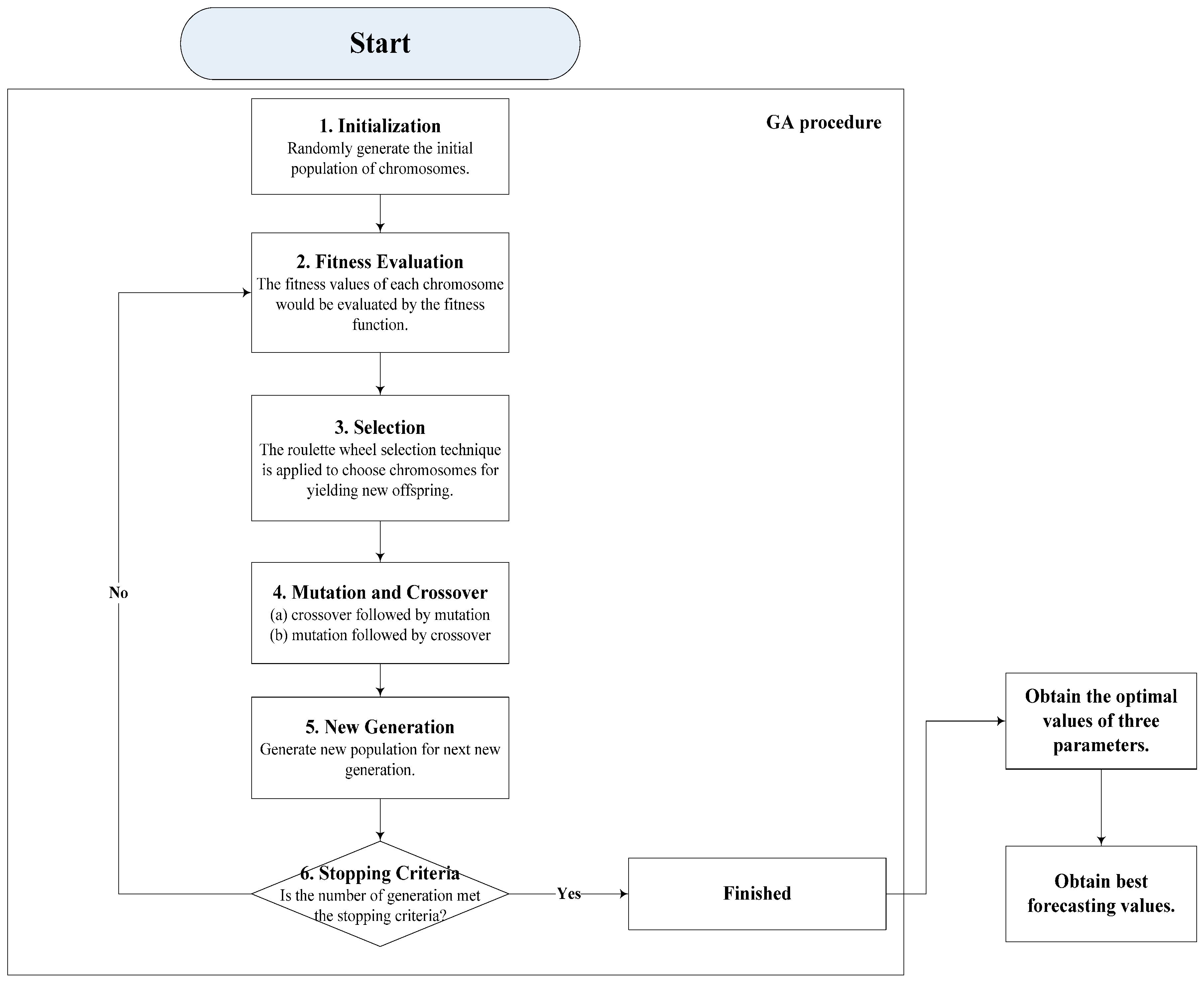
2.4. Genetic Algorithm (GA)
Genetic algorithm is the most famous evolutionary algorithm. Its primary concept is its elitist selection principle to keep best gene to be well survival from generation to generation during the evolutionary process in the natural systems. GA has several important operations, including selection, crossover, and mutation, to generate new individuals. It is able to effectively avoid trapping into local optima if more satisfied objective values could be successfully found. GA has been applied in many optimization problems.
The procedure of SVR-GA is briefly demonstrated as following steps and illustrated in Figure 2. Interested readers could refer to [27] for more detail.
- Step 1
- Initialization. Randomly generate the initial population of chromosomes.
- Step 2
- Fitness Evaluation. The fitness values of each chromosome would be evaluated by the fitness function. Similarly, in SVR-GA modeling process, MAPE and RMSE are used to measure the fitness (i.e., forecasting errors), and a switching between MAPE and RSME is also employed to ensure the smallest objective values could be selected.
- Step 3
- Selection. Elitism policy is employed while selecting good chromosomes, which receive satisfied fitness values for yielding new offspring in the next generation. Practically, the useful roulette wheel selection technique is applied to choose chromosomes for yielding new offspring.
- Step 4
- Mutation and Crossover. For crossover operation, this paper uses the single point technique, i.e., any paired chromosomes are exchanged at the same breaking points. For mutation operation, it is implemented randomly. The both techniques in GA, i.e., (a) crossover followed by mutation, and (b) mutation followed by crossover are tested in both of the series. In this paper, the rates of crossover and mutation operations are set as 0.8 and 0.05, as Hong et al. [26] suggested, respectively.
- Step 5
- New Generation. Generate new population for next new generation.
- Step 6
- Stopping Criterion. If the number of generation meets the stopping criterion, the current chromosome should be the best solution; otherwise, get back to Step 2 and repeat the procedure.
2.5. The Complete Processes of the Proposed Model
The complete processes of the proposed EMD-PSO-GA-SVR model is indicated as follows, the associate total flowchart is demonstrated in Figure 3.
- Step 1
- Data Decomposed. Apply the EMD technique to decompose the load data (training data) into intrinsic mode functions (IMFs) with higher and lower frequency parts, respectively. The details could be found in Section 2.1.
- Step 2
- Higher Frequency IMFs Modeling (by SVR-PSO). Higher frequency IMFs are modeled by an SVR model, and, as abovementioned that its parameters are determined by the PSO algorithm. Most suitable parameter combinations will be finalized with only the smallest forecasting errors (i.e., smallest MAPE value). The modeling details could be found in the relevant Section 2.2 and Section 2.3, and Figure 1.
- Step 3
- Lower Frequency IMFs Modeling (by SVR-GA). On the contrary, lower frequency IMFs are modeled by an SVR model, and, its parameters are determined by the GA algorithm. Similarly, only with smallest MAPE value, the associate parameters in the SVR model will be determined to be the most suitable combination. The relevant details could be referred Section 2.4 and Figure 2.
- Step 4
- EMD-PSO-GA-SVR Modeling. While the forecasting values for higher and lower frequencies IMFs have been calculated, respectively, then, the final forecasting results will also be performed.
3. Experimental Examples
Two experimental examples are used to demonstrate the advantages of the proposed model in terms of applicability, superiority, and generality. The data of the first example (Example 1, in Section 3.1) is obtained from Australian New South Wales (NSW) electricity market; the data of the second example (Example 2, in Section 3.2) is from American New York Independent System Operator (NYISO). Furthermore, to demonstrate the overtraining effect for different data sizes, in this paper, two kinds of data sizes, i.e., small data size and large data size, are employed to modeling and analysis, respectively.
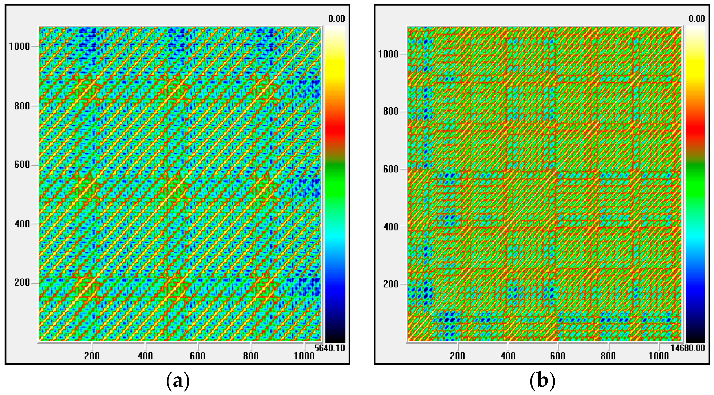
To ensure the feasibility of employing EMD to decompose the target data sets (both Examples 1 and 2) into higher and lower frequent parts, it is necessary to verify whether they are nonlinear and non-stationary. This paper applies the recurrence plot (RP) theory [36,37] to analyze these two characteristics. As it is known that RP reveals all of the times when the phase space trajectory of the dynamical system visits roughly the same area in the phase space, therefore, it is suitable to analyze the nonlinear and non-stationary characteristics of a data set. The RP analysis for Examples 1 and 2, as shown in Figure 4a,b, indicate: (1) it is clearly to see the parallel diagonal lines in both figures, i.e., both data sets reveal periodicity and deterministic, and this is the reason that authors could use these data sets to conduct forecasting; (2) it is also clearly to see the checkerboard structures in both figures, i.e., both data sets reveal that, after a transient, they go into slow oscillations that are superimposed on the chaotic motion; and, (3) it obviously demonstrates that vertical and horizontal lines cross at the cross, both data sets reveal laminar states, i.e., non-stationary characteristics. The relevant recurrence rate (the lower rate implies the nonlinear characteristic) and laminarity (the smaller value represents the non-stationary characteristic) for these two data sets also support the abovementioned RP analysis results. Based on the RP analysis, both the electricity load data set demonstrate macroscopic periodicity tendency (i.e., lower frequent part) and the microscopic chaotic oscillations tendency (i.e., higher frequent part), therefore, it is useful to employ EMD to decompose these two data sets into higher and lower frequent part, respectively.
3.1. The Forecasting Results of Example 1
3.1.1. Data Sets for Small and Large Sizes
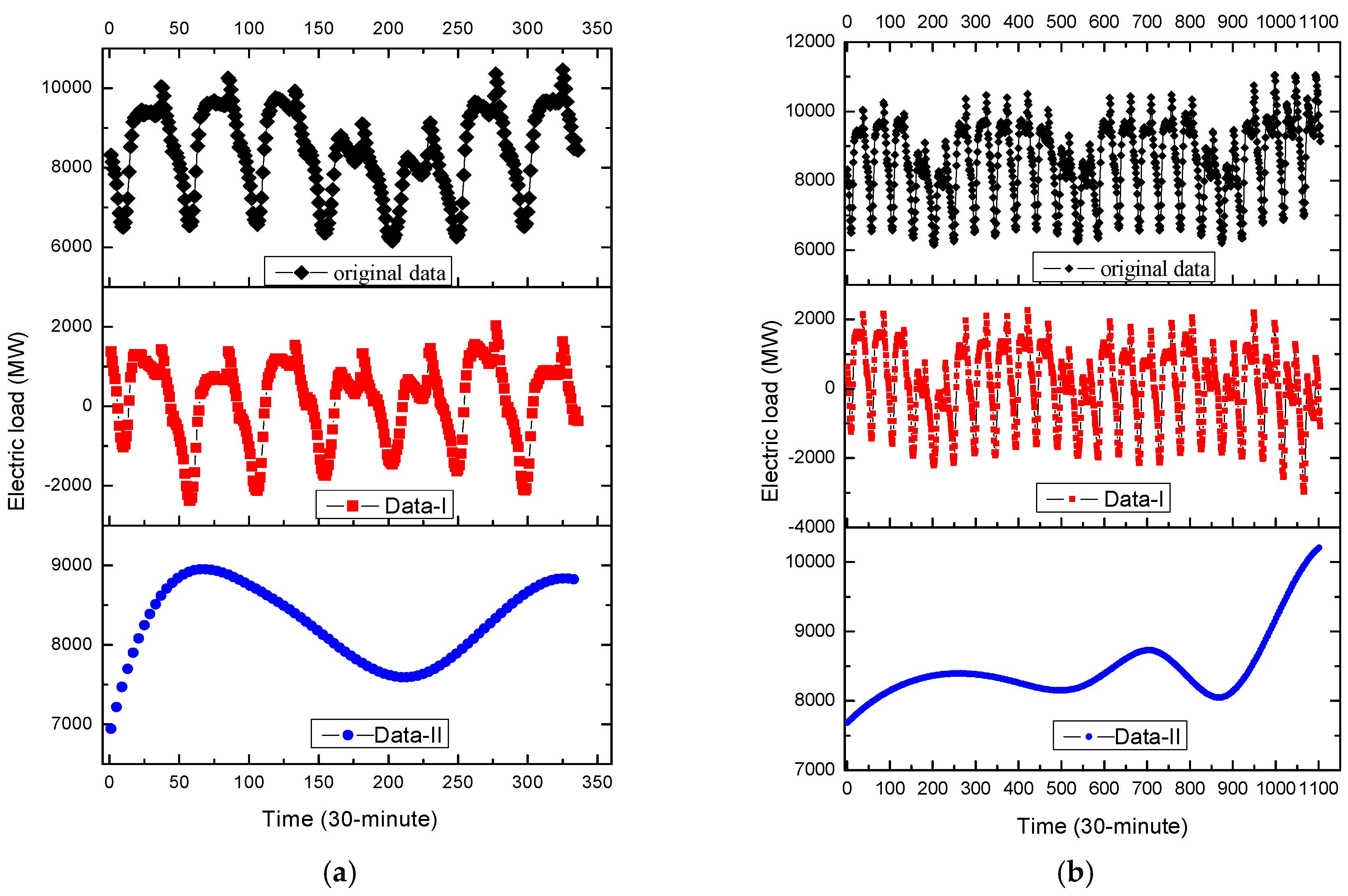
In Example 1, for small data size, there are totally 336 electricity load data per 30 min for seven days, i.e., from 2 to 8 May 2007. In which, the former 288 load data are used as the training data set, the latter 48 load data are as testing data set. The original data set is shown in Figure 5a.
On the other hand, for large data size, there are totally 1104 electricity load data from 2 to 24 May 2007, based on 30-min scale. In which, the former 768 load data (i.e., from 2 to 17 May 2007) are used as the training data set, the remainder 336 load data are used as the testing data set. The original data set is shown in Figure 5b.
3.1.2. Decomposition Results by EMD
The EMD is employed to decompose the original data set into higher and lower frequency items. For small data size, it could be divided into eight groups, as demonstrated in Figure 6a–h. In the meanwhile, the time delay of the data set in RP analysis (which value is 4) is simultaneously considered to select the higher and lower frequent parts. Consequently, the former four groups with much more frequency are classified as higher frequency items; the continued four groups with less frequency are classified as lower frequency items. The latest figure represents the original data; by the way, Figure 6h represents the trend term (i.e., residuals). As also shown in Figure 5a,b, the fluctuation characteristics of higher frequency item (namely Data-I) are almost the same with the original data, on the contrary, the macrostructure of lower frequency item (namely Data-II) is more stable. Data-I and Data-II will be further analyzed by SVR-PSO and SVR-GA models, respectively, to receive satisfied regression results. The details are illustrated in the next sub-section.
3.1.3. SVR-PSO for Data-I
As shown in Figure 5, Data-I almost presents as periodical stability every 24 h, which is consistent with people’s production and life. It also reflects the details of continuous changes. In this sub-section, SVR model is employed to conduct forecasting of Data-I, and as it is known that SVR requires evolutionary algorithms to appropriately determine its parameters to improve its forecasting accurate level. When considering that PSO is capable of solving the parameter determination problem from the data set with mentioned continuous change details, therefore, PSO is applied to be hybridized with the SVR model to forecast Data-I.
Firstly, the higher frequency items (i.e., Data-I) from small and large data sizes are both used for SVR-PSO modeling. Then, the best modeled results in training and testing stages are received, as shown in Figure 7a,b, respectively. As demonstrated in Figure 7, it is obvious to learn about the forecasting accuracy improvements from the hybridization of PSO.
3.1.4. SVR-GA for Data-II
As shown in Figure 6e–h, the lower frequency item has not only less frequency, but also demonstrates more stability, particularly for the residuals, Figure 6h. In addition, in the long term, there would suffer from nonlinear mechanical changes, which are relatively discrete. In this sub-section, the SVR model is also used to conduct forecasting of Data-II, and also requires appropriate algorithm to well determine its three parameters. Therefore, it is more suitable to apply GA, while the SVR model is modeling. As abovementioned, GA is familiar to solve discrete problems, thus, the parameters settings of the SVR model for small and large data sizes are the same as shown in Table 3.
Similarly, the lower frequency items (i.e., Data-II) from small and large data sizes are used for SVR-GA modeling. Then, the best modeled results in training and testing stages are received, as shown in Figure 8a,b, respectively. In which, it has demonstrated the superiority from the hybridization of GA. The determined parameters of the SVR-GA model are shown in Table 4.
3.2. The Forecasting Results of Example 2
3.2.1. Data Sets for Small and Large Sizes
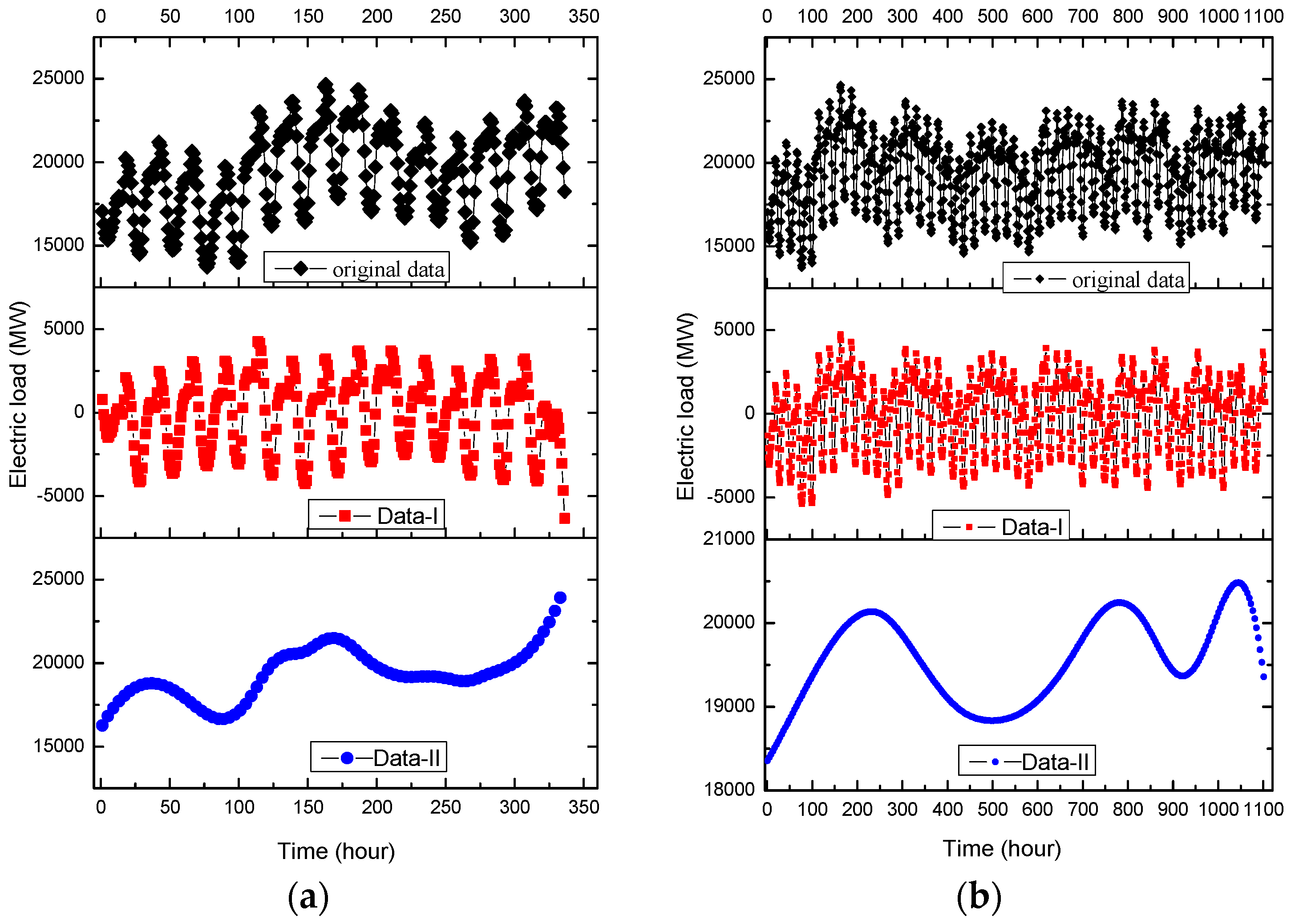
In Example 2, small data size, also totaling 336 hourly load data for 14 days (from 1 to 14 January 2015) are collected. In which, the former 288 load data are used as the training data set, the latter 48 load data are as testing data set. The original data set is shown in Figure 9a.
For large data size, totally 1104 hourly load data for 46 days (from 1 January to 15 February 2015) are collected to model. The former 768 load data are employed as the training data set, and the remainder 336 load data are used as the testing data set. The original data set is illustrated in Figure 9b.
3.2.2. Decomposition Results by EMD
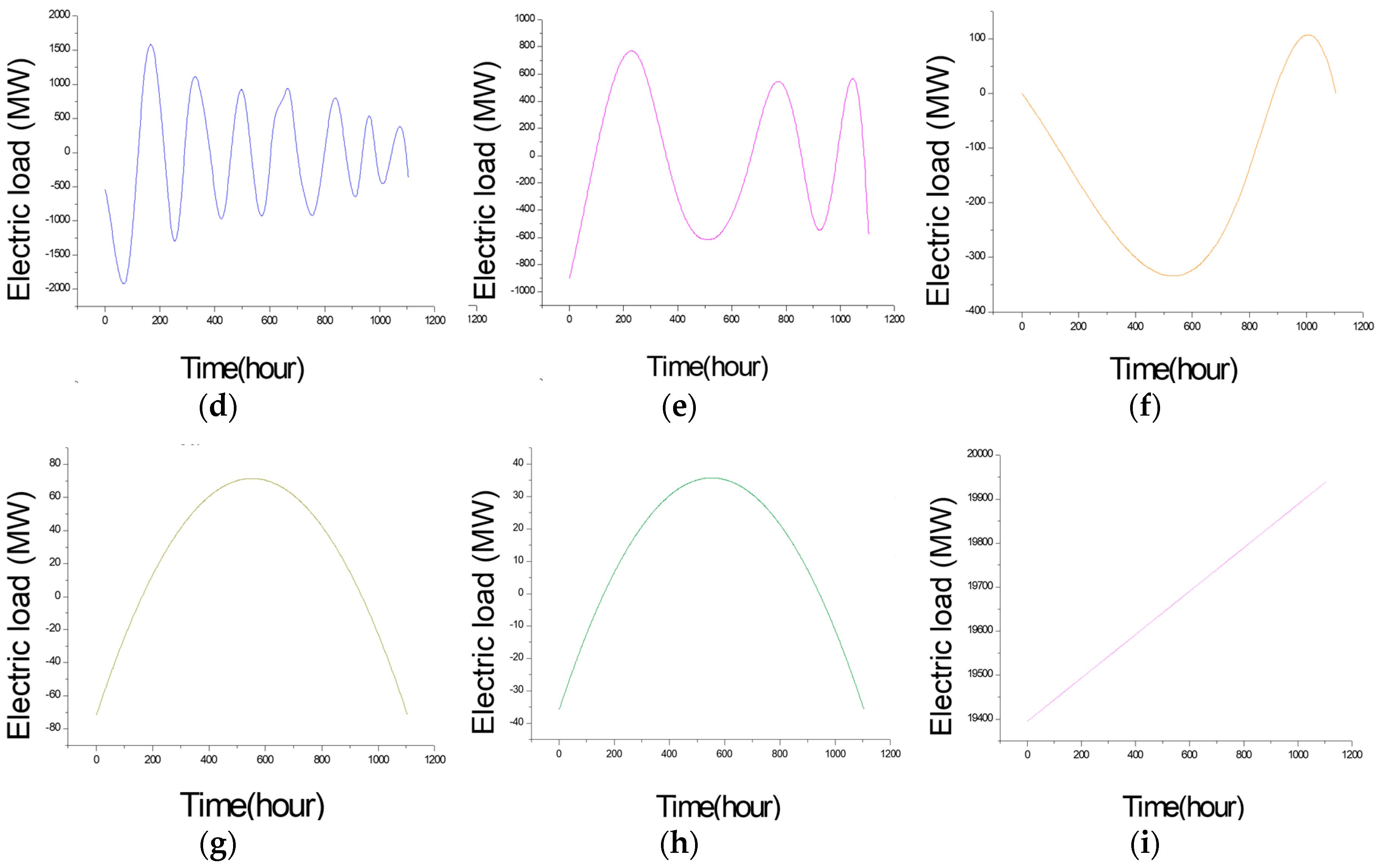
Similar as in Example 1, EMD is used to decompose the original data set into higher and lower frequency items. For small data size, it could be divided into nine groups, as shown in Figure 10a–i. In the meanwhile, the time delay of the data set in RP analysis (which value is 4) is simultaneously considered to select the higher and lower frequent parts. Consequently, the former five groups with much more frequency are classified as higher frequency items; the continued four groups with less frequency are classified as lower frequency items. Figure 10i also represents the trend term (i.e., residuals). The fluctuation characteristics of Data-I are also obviously the same as the original data, as demonstrated in Figure 9a,b. On the contrary, the macrostructure of Data-II is more stable. Data-I and Data-II will also be further analyzed by SVR-PSO and SVR-GA models, respectively, to receive satisfied regression results.
3.2.3. SVR-PSO for Data-I
As shown in Figure 9, Data-I also presents as periodical stability every 24 h, which is the same with the original data. Therefore, it is as similar as in Example 1, PSO is applied to be hybridized with the SVR model to forecast the Data-I.
Firstly, the higher frequency items (i.e., Data-I) from small and large data sizes are both used for SVR-PSO modeling. The best modeled results in the training and testing stages are received, as shown in Figure 11a,b, respectively. In which, it is obvious to observe that the forecasting accuracy improvements from the hybridization of PSO. The parameters settings of the SVR model for small and large data sizes are as the same as in Example 1, i.e., as shown in Table 1; the determined parameters of the SVR-PSO model are illustrated Table 5.
3.2.4. SVR-GA for Data-II
As shown in Figure 10f–i, the lower frequency item (i.e., Data-II) has less frequency and stability. Therefore, it is as the same as in Example 1, GA is also hybridized with the SVR model to forecast the Data-II. The parameters settings of the SVR model for small and large data sizes are also as the same as shown in Table 3. The best modeled results in training and testing stages are received, as shown in Figure 12a,b, respectively. In which, it has demonstrated the superiority from the hybridization of GA. The determined parameters of the SVR-GA model are shown in Table 6.
4. Forecasting Results and Analyses
This section will completely address the forecasting results of these two employed examples with two data sizes and associate higher and lower frequency items (Data-I and Data-II), to further demonstrate the efficiency of the proposed EMD-PSO-GA-SVR model in terms of forecasting accuracy and interpretability.
4.1. Forecasting Accuracy Evaluation Indexes
To completely reflect the forecasting performances of the proposed model, three representative forecasting accuracy evaluation indexes are employed to conduct the evaluation. Except the mean absolute percentage error (MAPE) and the root mean square error (RMSE), as introduced in Equations (16) and (17), the other one is the mean absolute error (MAE), which is calculated by Equation (18),
where is the actual load value at point i; is the forecasted load value at point i; and, N is the total number of data.
In addition, two famous criteria for model selection among a finite set of models, i.e., Akaike information criterion (AIC) [38,39] and Bayesian information criterion (BIC) [39,40], are employed to further compare which model performs (fits) better. The AIC estimates the quality of each of the collected models for fitting the data, relative to each of the other models. The AIC value of the selected model is calculated as Equation (19). During the model fitting processes, it is possible to increase the accuracy by adding parameters, and it eventually results in overfitting problems. The BIC value of the selected model is calculated as Equation (20).
The model with the lowest AIC and BIC is preferred. They both attempt to resolve the overfitting problem by introducing a penalty term for the number of parameters in the model.
where N is the total number of data; k is the number of parameters in a model.
4.2. Forecasting Performances
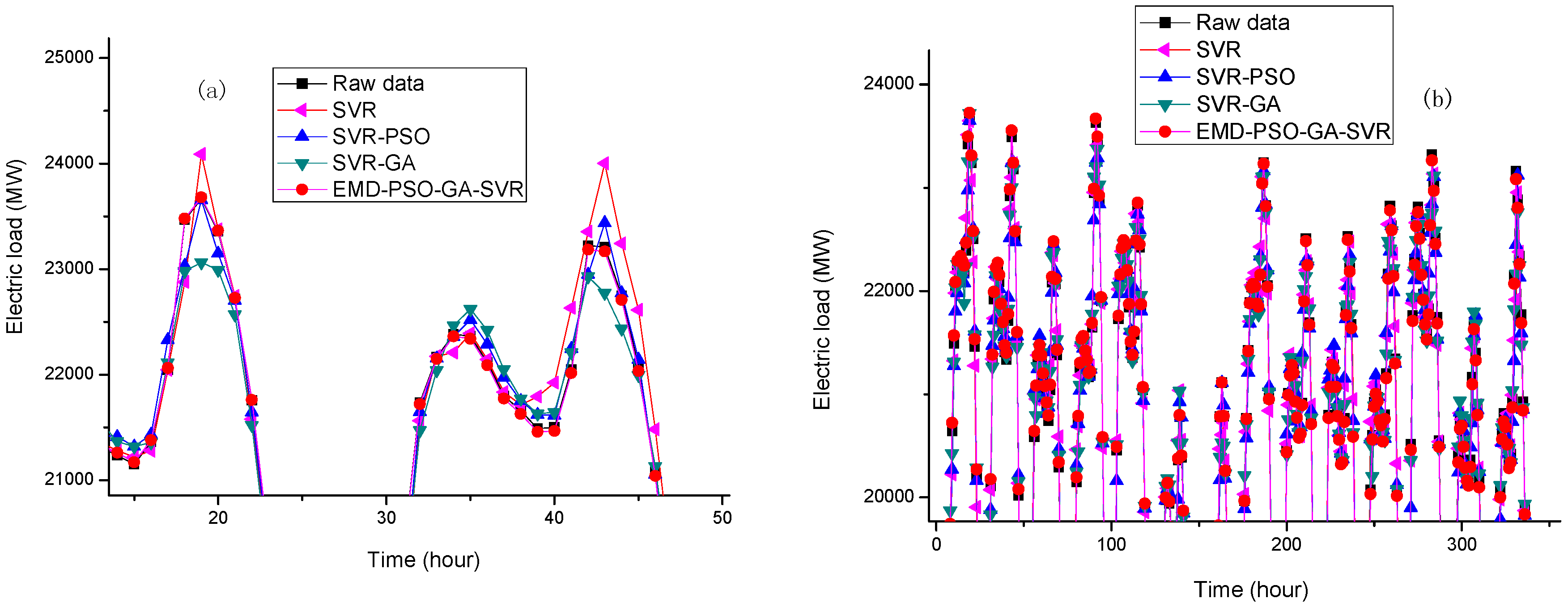
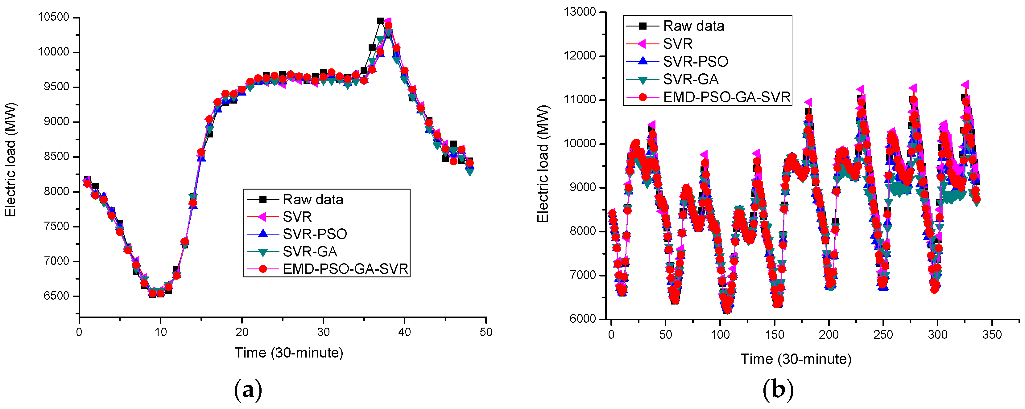
In Example 1, the forecasting performances of the proposed EMD-PSO-GA-SVR model for small data size and large data size are illustrated in Figure 13, in which other competitive models are also shown, such as the original SVR model, SVR-PSO model, and SVR-GA model. Figure 13 demonstrates clearly that the proposed model provides better fitness than other competitive models for both small and large data sizes.
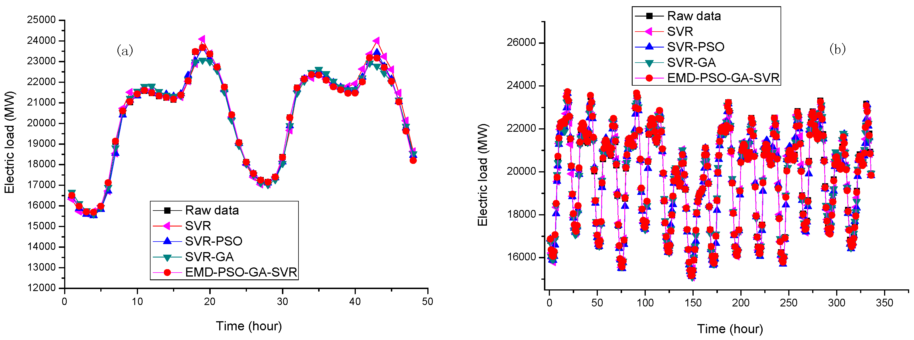
In Example 2, for both small and large data sizes, the forecasting performances of the proposed model and other competitive models are shown in Figure 14. Once again, the proposed model also receives better fitness, particularly within the period peak loads occurs, i.e., the proposed EMD-PSO-GA-SVR model demonstrates a better generalization capability than other competitive models. To verify this result clearly, the local enlargement around the period of peak load in Figure 14a,b are enlarged in Figure 15a,b, respectively. It is shown that the extraction of microscopic detail can express its periodic characteristics very well, and the macroscopic structure is also in the lower frequency range. The discretization characteristic is expressed by GA, especially at the sharp point; in addition, 24-h periodicity has also been reflected. It is clearly to learn that the forecasting curve of the proposed model can fit closer to the actual load curve than other competitive models. It is powerful to capture the changing tendency of the data, including the nonlinear fluctuation tendency.
The forecasting detail results in both Examples 1 and 2 are listed in Table 7 and Table 8, respectively. When comparing the proposed EMD-PSO-GA-SVR model with other competitive models, it could be found that the proposed model is superior in terms of all of the forecasting performance evaluation indexes. Therefore, it could be concluded that the proposed model performs with effectiveness and efficiency more than other competitive models, and eventually, the proposed hybrid model could receive better forecasting accuracy levels and statistical interpretation. Particularly, as illustrated in Figure 15, the proposed model demonstrates a higher fitness capability and excellent flexibility during the period of peak point or inflection point, due to capturing redundant information by GA in the modeling process, and by significantly increasing the forecasting accurate level.
Some advantages of the proposed model could be concluded based on the forecasting performances, as abovementioned. The first one should be that the proposed model is superior to other competitive models based on the comparisons (Figure 14 and Figure 15, Table 7 and Table 8). Secondly, based on Figure 14 and Figure 15 in Example 2, the proposed EMD-PSO-GA-SVR model has been trained to receive a better generalization ability while dealing with different input patterns. In addition, based on the forecasting performance comparisons from small and large data sizes in Examples 1 and 2, the proposed model is capable learning about more redundant information and to successfully model the model with large data size. Eventually, as illustrated in Table 7 and Table 8, the proposed model performance satisfied forecasting accuracy and well interpretability parameters, i.e., the robustness and effectiveness are received. Thus, the proposed model is a remarkable approach to easily forecast electricity load. Particularly, in terms of AIC and BIC criteria, the proposed model also receives smallest values of AIC and BIC than the other competitive models, it indicates that the proposed model fits better and avoid overfitting problems.
Finally, to ensure the significance of forecasting accuracy improvements among the proposed model and other competitive models, a statistical test, namely Wilcoxon signed-rank test, is implemented at the 0.05 significant level under one-tail-test. The test results are illustrated in Table 9. Obviously, the proposed model outperforms the other competitive models significantly.
5. Conclusions
This paper proposes a novel SVR-based electricity load forecasting model, by hybridizing EMD to decompose the time series data set into higher and lower frequency parts, and, by hybridizing PSO and GA algorithms to determine the three parameters of the SVR models for these two parts, respectively. Via two experimental examples from Australian and American electricity market open data sets, the proposed EMD-PSO-GA-SVR model receives significant forecasting performances rather than other competitive forecasting models in published papers, such as original SVR, SVR-PSO, SVR-GA, and AFCM models.
The most significant contribution of this paper is to overcome the practical drawbacks of an SVR model: the SVR model could only provide poor forecasting for other data patterns, if it is over trained to some data pattern with overwhelming size. Authors firstly apply EMD to decompose the data set into two sub-sets with different data patterns, the higher frequency part and the lower frequency part, to take into account both the accuracy and interpretability of the forecast results. Secondly, authors employ two suitable evolutionary algorithms to reduce the performance volatility of an SVR model with different parameters. PSO and GA are implemented to determine the parameter combination during the SVR modeling process. The results indicate that the proposed EMD-PSO-GA-SVR model demonstrates a better generalization capability than the other competitive models in terms of forecasting capability. It is shown that the extraction of microscopic detail can express its periodic characteristics well, and the macroscopic structure is also in the lower frequency range. The discretization characteristic is expressed by GA, especially at the sharp point, i.e., GA can effectively capture the exact sharp characteristics while the embedded effects of noise and the other factors intertwined. Eventually receiving more satisfying forecasting performances than the other competitive models.
Acknowledgments
This paper is sponsored by the Start-up Foundation for Doctors (No. PXY-BSQD-2014001), Educational Commission of Henan Province of China (No. 15A530010), The Youth Foundation of Ping Ding Shan University (No. PXY-QNJJ-2014008), Jiangsu Distinguished Professor Project by Jiangsu Provincial Department of Education, and Ministry of Science and Technology, Taiwan (MOST 106-2221-E-161-005-MY2).
Author Contributions
Guo-Feng Fan and Wei-Chiang Hong conceived and designed the experiments; Li-Ling Peng and Xiangjun Zhao performed the experiments; Guo-Feng Fan and Wei-Chiang Hong analyzed the data and wrote the paper.
Conflicts of Interest
The authors declare no conflict of interest.
References
- Li, Z.; Hurn, A.S.; Clements, A.E. Forecasting quantiles of day-ahead electricity load. Energy Econ. 2017, 67, 60–71. [Google Scholar] [CrossRef]
- Arora, S.; Taylor, J.W. Rule-based autoregressive moving average models for forecasting load on special days: A case study for France. Eur. J. Oper. Res. 2017. [Google Scholar] [CrossRef]
- Takeda, H.; Tamura, Y.; Sato, S. Using the ensemble Kalman filter for electricity load forecasting and analysis. Energy 2016, 104, 184–198. [Google Scholar] [CrossRef]
- Zhao, H.; Guo, S. An optimized grey model for annual power load forecasting. Energy 2016, 107, 272–286. [Google Scholar] [CrossRef]
- Dedinec, A.; Filiposka, S.; Dedinec, A.; Kocarev, L. Deep belief network based electricity load forecasting: An analysis of Macedonian case. Energy 2016, 115, 1688–1700. [Google Scholar] [CrossRef]
- Mordjaoui, M.; Haddad, S.; Medoued, A.; Laouafi, A. Electric load forecasting by using dynamic neural network. Int. J. Hydrogen Energy 2017, 42, 17655–17663. [Google Scholar] [CrossRef]
- Khwaja, A.S.; Zhang, X.; Anpalagan, A.; Venkatesh, B. Boosted neural networks for improved short-term electric load forecasting. Electr. Power Syst. Res. 2017, 143, 431–437. [Google Scholar] [CrossRef]
- Hua, R.; Wen, S.; Zeng, Z.; Huang, T. A short-term power load forecasting model based on the generalized regression neural network with decreasing step fruit fly optimization algorithm. Neurocomputing 2017, 221, 24–31. [Google Scholar] [CrossRef]
- Mahmoud, T.S.; Habibi, D.; Hassan, M.Y.; Bass, O. Modelling self-optimised short term load forecasting for medium voltage loads using tunning fuzzy systems and artificial neural networks. Energy Convers. Manag. 2015, 106, 1396–1408. [Google Scholar] [CrossRef]
- Bessec, M.; Fouquau, J. Short-run electricity load forecasting with combinations of stationary wavelet transforms. Eur. J. Oper. Res. 2018, 264, 149–164. [Google Scholar] [CrossRef]
- Zeng, N.; Zhang, H.; Liu, W.; Liang, J.; Alsaadi, F.E. A switching delayed PSO optimized extreme learning machine for short-term load forecasting. Neurocomputing 2017, 240, 175–182. [Google Scholar] [CrossRef]
- Liu, N.; Tang, Q.; Zhang, J.; Fan, W.; Liu, J. A hybrid forecasting model with parameter optimization for short-term load forecasting of micro-grids. Appl. Energy 2014, 129, 336–345. [Google Scholar] [CrossRef]
- Kouhi, S.; Keynia, F.; Ravadanegh, S.N. A new short-term load forecast method based on neuro-evolutionary algorithm and chaotic feature selection. Int. J. Electr. Power Energy Syst. 2014, 62, 862–867. [Google Scholar] [CrossRef]
- Bahrami, S.; Hooshmand, R.-A.; Parastegari, M. Short term electric load forecasting by wavelet transform and grey model improved by PSO (particle swarm optimization) algorithm. Energy 2014, 72, 434–442. [Google Scholar] [CrossRef]
- An, X.; Jiang, D.; Liu, C.; Zhao, M. Wind farm power prediction based on wavelet decomposition and chaotic time series. Expert Syst. Appl. 2011, 38, 11280–11285. [Google Scholar] [CrossRef]
- Hung, W.M.; Hong, W.C. Application of SVR with improved ant colony optimization algorithms in exchange rate forecasting. Control Cybern. 2009, 38, 863–891. [Google Scholar]
- Hong, W.C. Traffic flow forecasting by seasonal SVR with chaotic simulated annealing algorithm. Neurocomputing 2011, 74, 2096–2107. [Google Scholar] [CrossRef]
- Pai, P.F.; Hong, W.C. A recurrent support vector regression model in rainfall forecasting. Hydrol. Process 2007, 21, 819–827. [Google Scholar] [CrossRef]
- Hong, W.C. Intelligent Energy Demand Forecasting; Springer: London, UK, 2013. [Google Scholar]
- An, X.; Jiang, D.; Zhao, M.; Liu, C. Short-term prediction of wind power using EMD and chaotic theory. Commun. Nonlinear Sci. Numer. Simul. 2012, 17, 1036–1042. [Google Scholar] [CrossRef]
- Huang, B.; Kunoth, A. An optimization based empirical mode decomposition scheme. J. Comput. Appl. Math. 2013, 240, 174–183. [Google Scholar] [CrossRef]
- Fan, G.; Qing, S.; Wang, S.Z.; Hong, W.C.; Dai, L. Study on apparent kinetic prediction model of the smelting reduction based on the time series. Math. Probl. Eng. 2012, 720849. [Google Scholar] [CrossRef]
- Premanode, B.; Toumazou, C. Improving prediction of exchange rates using differential EMD. Expert Syst. Appl. 2013, 40, 377–384. [Google Scholar] [CrossRef]
- Li, M.; Hong, W.-C.; Kang, H. Urban traffic flow forecasting using Gauss-SVR with cat mapping, cloud model and PSO hybrid algorithm. Neurocomputing 2013, 99, 230–240. [Google Scholar] [CrossRef]
- Hong, W.-C. Chaotic particle swarm optimization algorithm in a support vector regression electric load forecasting model. Energy Convers. Manag. 2009, 50, 105–117. [Google Scholar] [CrossRef]
- Hong, W.-C.; Dong, Y.; Zhang, W.; Chen, L.-Y.; Panigrahi, B.K. Cyclic electric load forecasting by seasonal SVR with chaotic genetic algorithm. Int. J. Electr. Power Energy Syst. 2013, 44, 604–614. [Google Scholar] [CrossRef]
- Chen, R.; Liang, C.; Hong, W.-C.; Gu, D. Forecasting holiday daily tourist flow based on seasonal support vector regression with adaptive genetic algorithm. Appl. Soft Comput. 2015, 26, 435–443. [Google Scholar] [CrossRef]
- Geng, J.; Huang, M.-L.; Li, M.-W.; Hong, W.-C. Hybridization of seasonal chaotic cloud simulated annealing algorithm in a SVR-based load forecasting model. Neurocomputing 2015, 151, 1362–1373. [Google Scholar] [CrossRef]
- Ju, F.-Y.; Hong, W.-C. Application of seasonal SVR with chaotic gravitational search algorithm in electricity forecasting. Appl. Math. Model. 2013, 37, 9643–9651. [Google Scholar] [CrossRef]
- Huang, Y.; Schmitt, F.G. Time dependent intrinsic correlation analysis of temperature and dissolved oxygen time series using empirical mode decomposition. J. Mar. Syst. 2014, 130, 90–100. [Google Scholar] [CrossRef]
- Vapnik, V.; Golowich, S.; Smola, A. Support vector machine for function approximation, regression estimation, and signal processing. Adv. Neural Inf. Process. Syst. 1996, 9, 281–287. [Google Scholar]
- Kennedy, J.; Eberhart, R.C. Particle swarm optimization. In Proceedings of the IEEE International Conference Neural Networks, Perth, Australia, 27 November–1 December 1995; pp. 1942–1948. [Google Scholar]
- Eberhart, R.C.; Shi, Y. Particle swarm optimization: Developments, applications and resources. In Proceedings of the 2001 Congress on Evolutionary Computation, Seoul, Korea, 27–30 May 2001; pp. 81–86. [Google Scholar]
- Sun, T.H. Applying particle swarm optimization algorithm to roundness measurement. Expert Syst. Appl. 2009, 36, 3428–3438. [Google Scholar] [CrossRef]
- Coelho, L.S. An efficient particle swarm approach for mixed-integer programming in reliability–redundancy optimization applications. Reliab. Eng. Syst. Saf. 2009, 94, 830–837. [Google Scholar] [CrossRef]
- Eckmann, J.P.; Kamphorst, S.O.; Ruelle, D. Recurrence plots of dynamical systems. Europhys. Lett. 1987, 5, 973–977. [Google Scholar] [CrossRef]
- Marwan, N.; Romano, M.C.; Thiel, M.; Kurths, J. Recurrence plots for the analysis of complex systems. Phys. Rep. 2007, 438, 237–329. [Google Scholar] [CrossRef]
- Akaike, H. A new look at the statistical model identification. IEEE Trans. Autom. Control 1974, 19, 716–723. [Google Scholar] [CrossRef]
- Aho, K.; Derryberry, D.; Peterson, T. Model selection for ecologists: The worldviews of AIC and BIC. Ecology 2014, 95, 631–636. [Google Scholar] [CrossRef] [PubMed]
- Schwarz, G.E. Estimating the dimension of a model. Ann. Stat. 1978, 6, 461–464. [Google Scholar] [CrossRef]
Figure 1.
Support vector regression (SVR)- particle swarm optimization (PSO) algorithm flowchart.
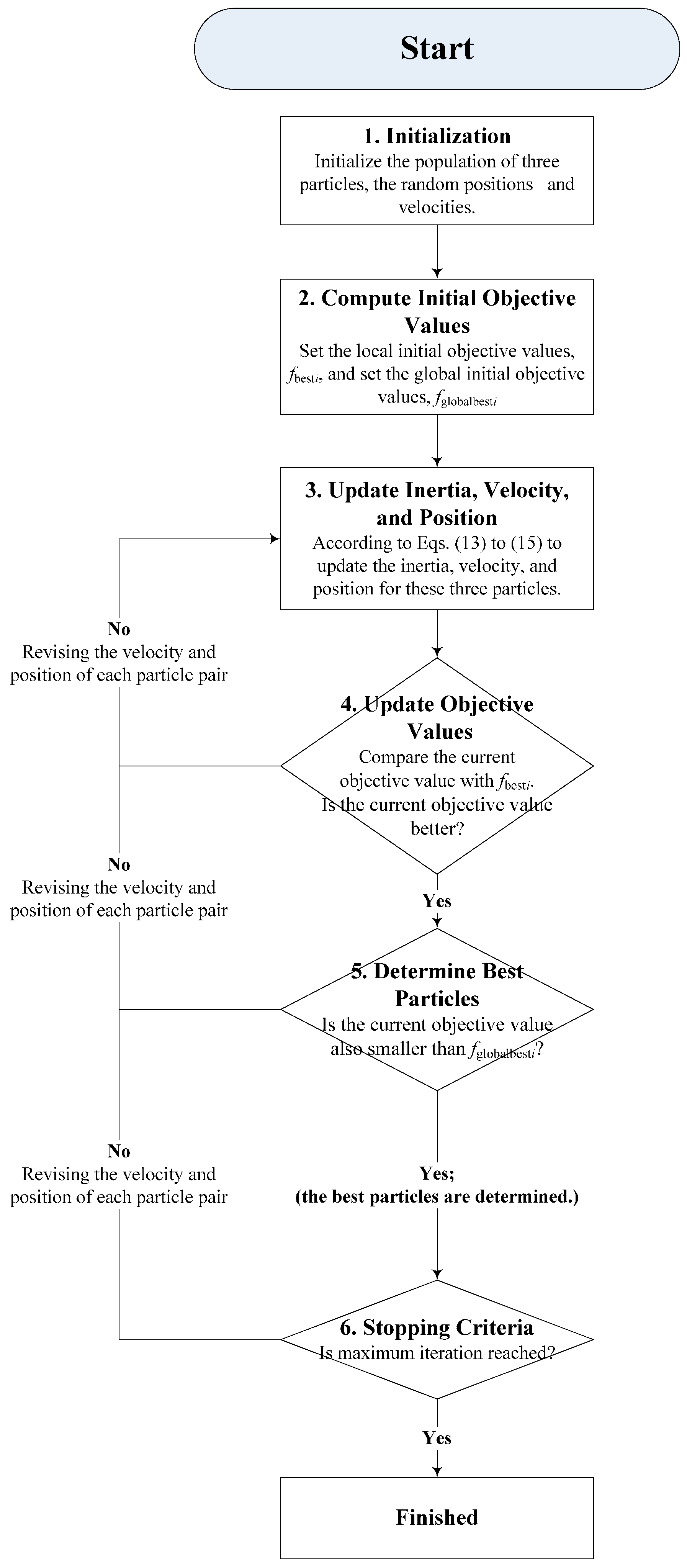
Figure 2.
SVR- genetic algorithm (GA) algorithm flowchart.

Figure 3.
The total flowchart of the proposed empirical mode decomposition (EMD)-PSO-GA-SVR model.
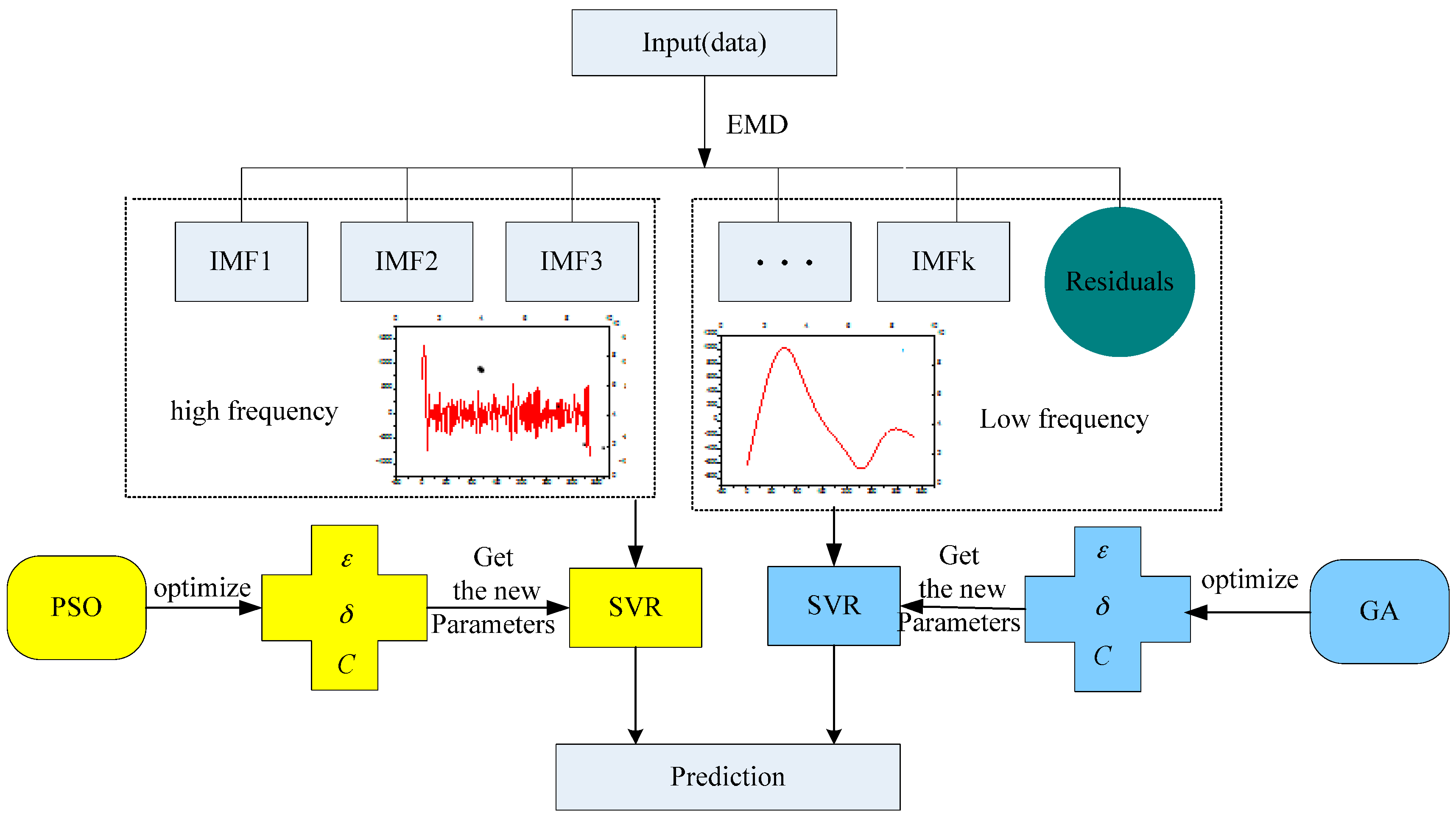
Figure 4.
The recurrence plot for Examples 1 and 2. (a) Example 1 embedding dimensions = 4; time delays = 13; recurrence rate = 33.3%; laminarity = 51.0% (Small data size from Australian New South Wales, NSW); (b) Example 2 embedding dimensions = 4; time delays = 4; recurrence rate = 38.1%; laminarity = 54.7% (Small data size from American New York Independent System Operator, NYISO).

Figure 5.
The 30-min based original data, Data-I, Data-II (Example 1). (a) Small data size (2–8 May 2007); (b) Large data size (2–24 May 2007).
Figure 5.
The 30-min based original data, Data-I, Data-II (Example 1). (a) Small data size (2–8 May 2007); (b) Large data size (2–24 May 2007).

Figure 6.
The decomposed different items for small data size (Example 1). (a) IMF (intrinsic modulo function) 1; (b) IMF 2; (c) IMF 3; (d) IMF 4; (e) IMF 5; (f) IMF 6; (g) IMF 7; (h) residuals; (i) the raw data.
Figure 6.
The decomposed different items for small data size (Example 1). (a) IMF (intrinsic modulo function) 1; (b) IMF 2; (c) IMF 3; (d) IMF 4; (e) IMF 5; (f) IMF 6; (g) IMF 7; (h) residuals; (i) the raw data.
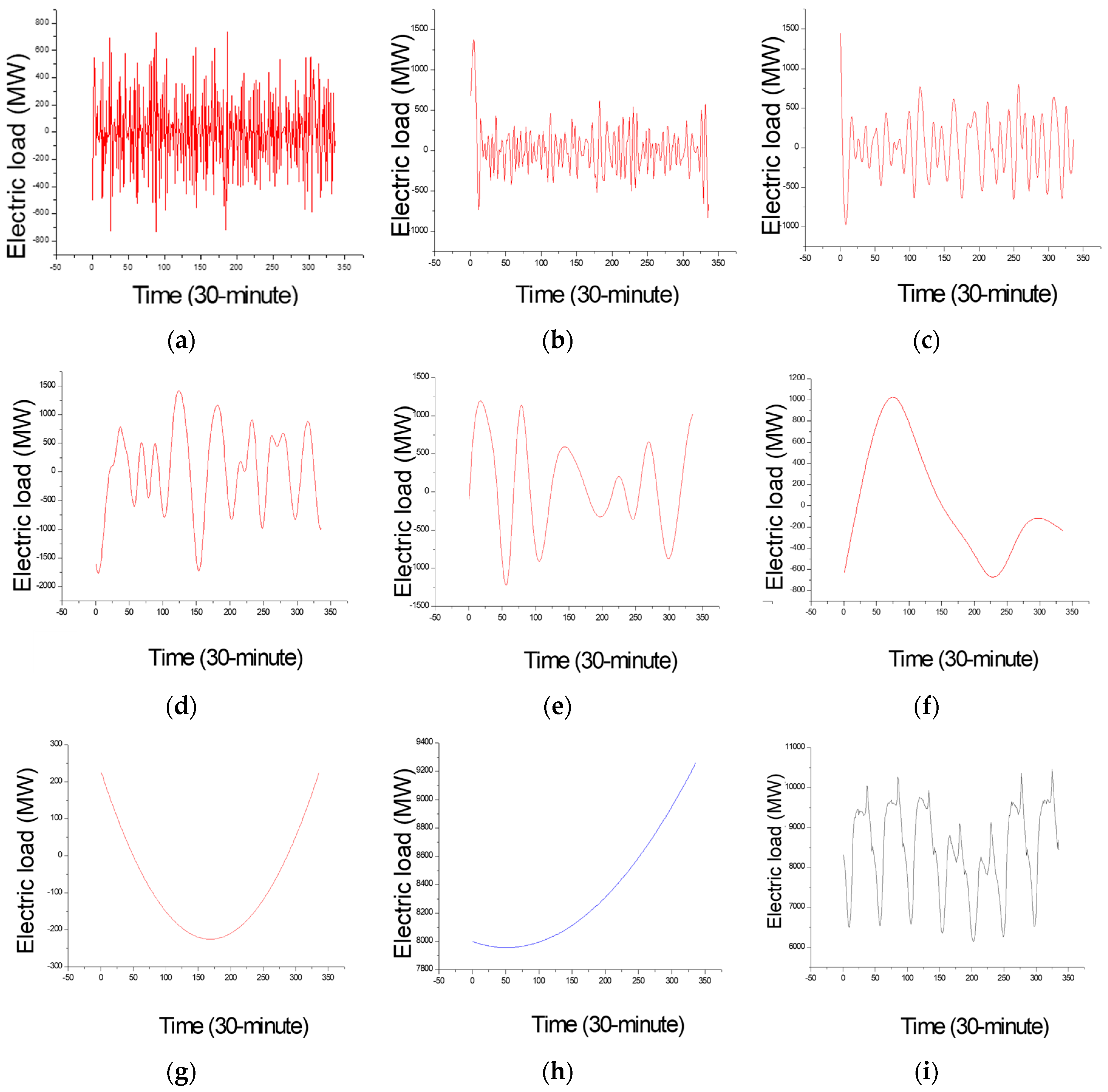
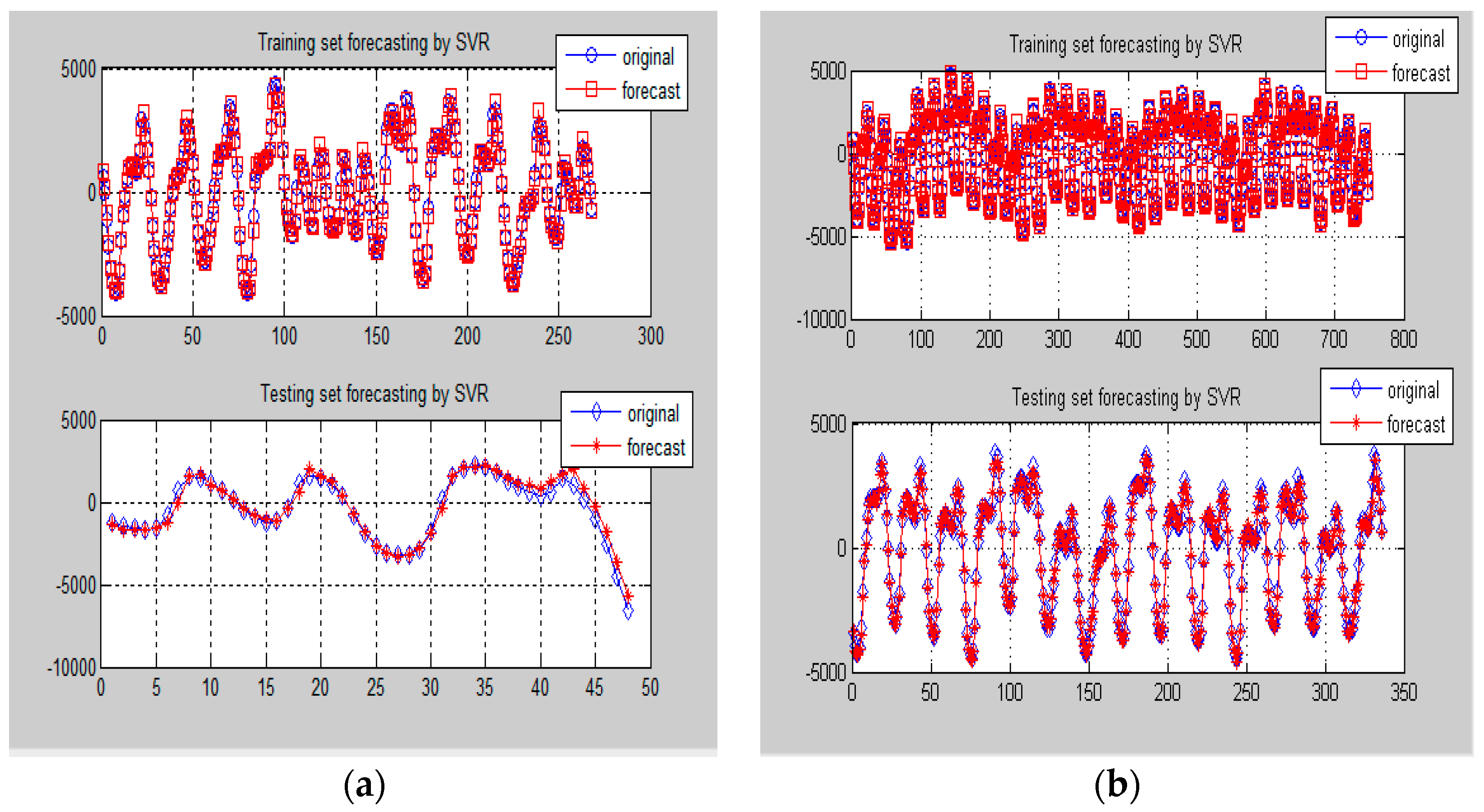
Figure 7.
Comparison of forecasting results by SVR-PSO model for Data-I (Example 1). (a) One-day ahead forecasting on 8 May 2007; (b) One-week ahead forecasting from 18 to 24 May 2007.
Figure 7.
Comparison of forecasting results by SVR-PSO model for Data-I (Example 1). (a) One-day ahead forecasting on 8 May 2007; (b) One-week ahead forecasting from 18 to 24 May 2007.
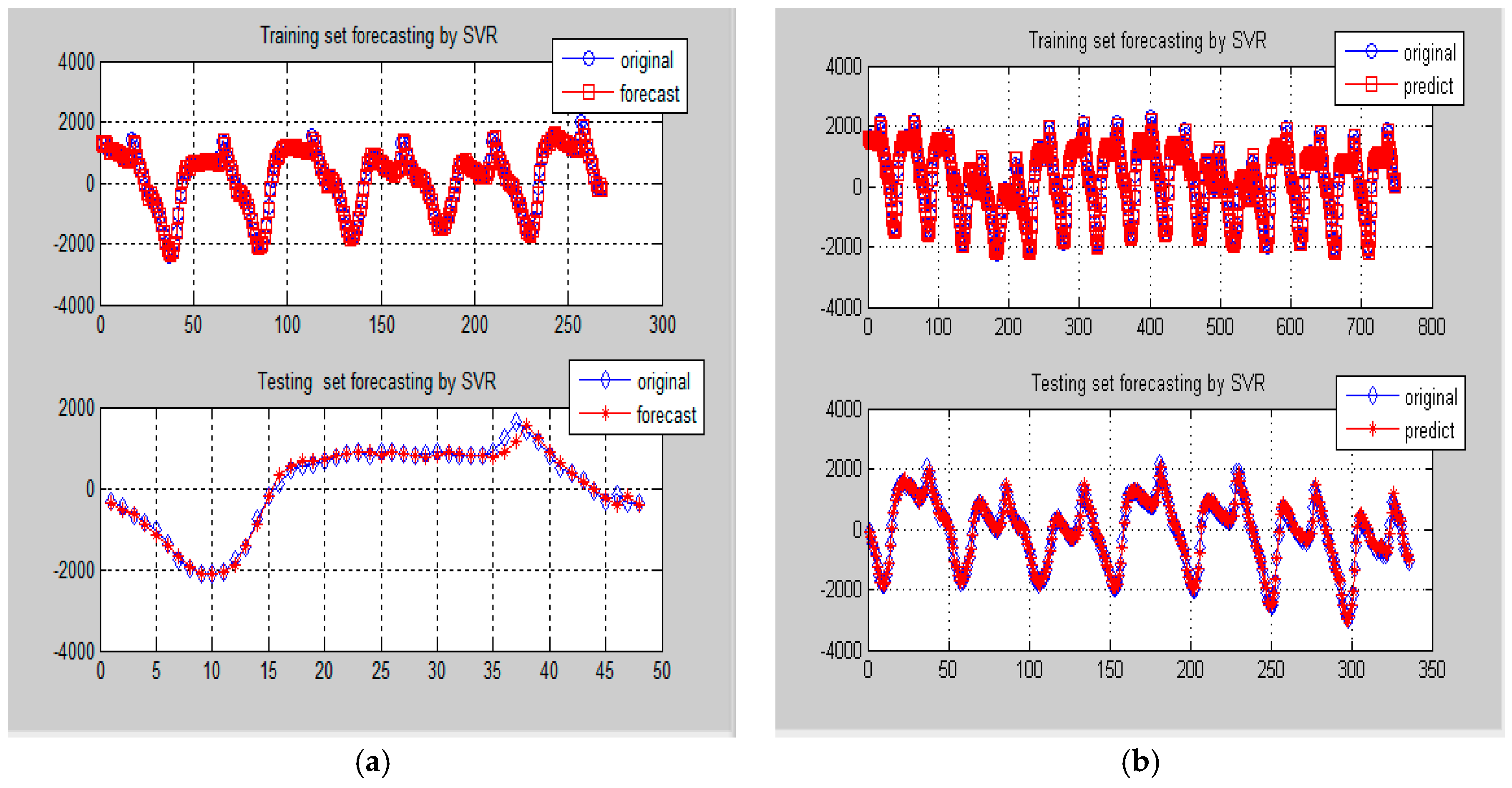
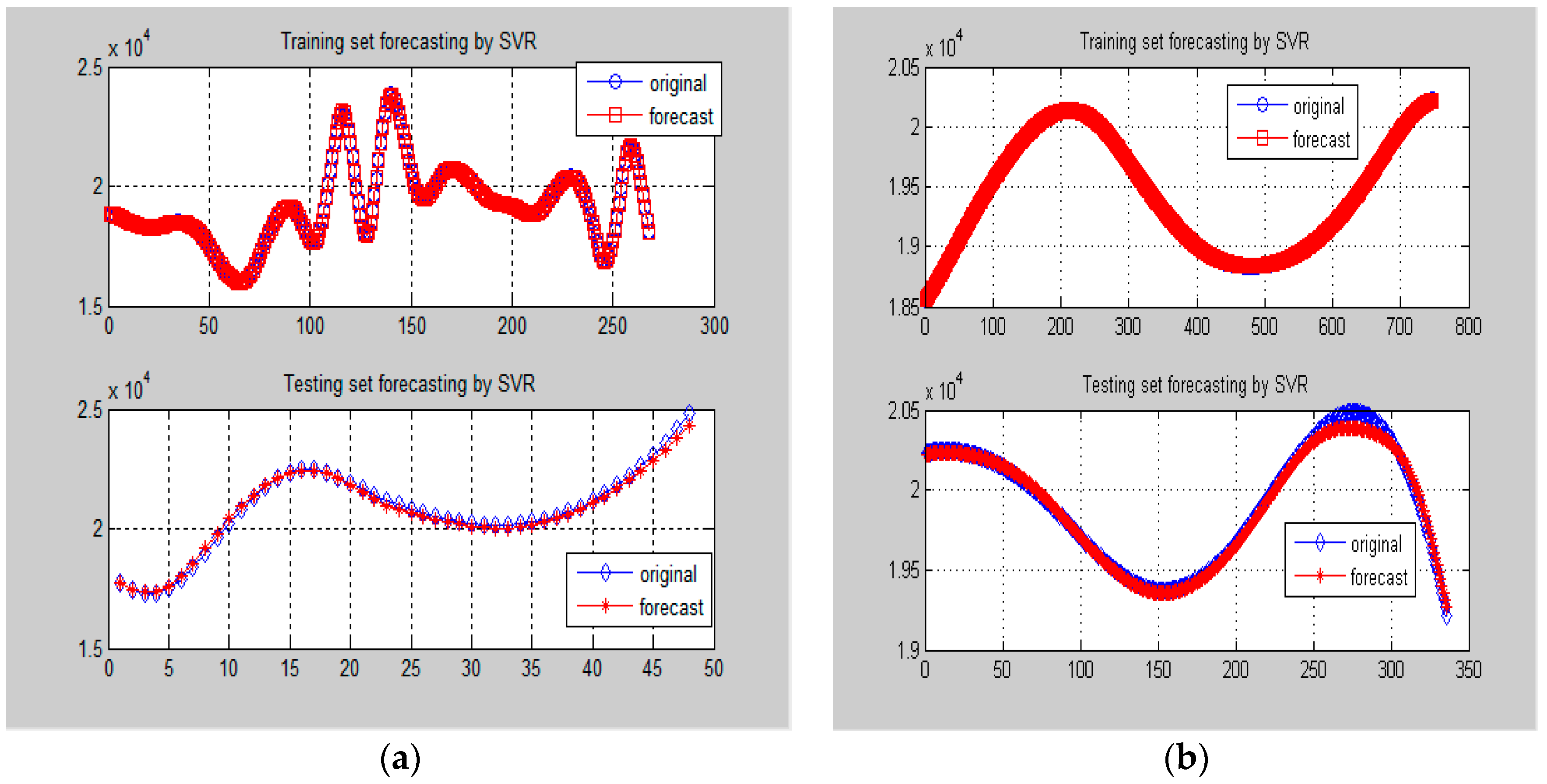
Figure 8.
Comparison of forecasting results by SVR-GA model for Data-II (Example 1). (a) One-day ahead forecasting on 8 May 2007; (b) One-week ahead forecasting from 18 to 24 May 2007.
Figure 8.
Comparison of forecasting results by SVR-GA model for Data-II (Example 1). (a) One-day ahead forecasting on 8 May 2007; (b) One-week ahead forecasting from 18 to 24 May 2007.
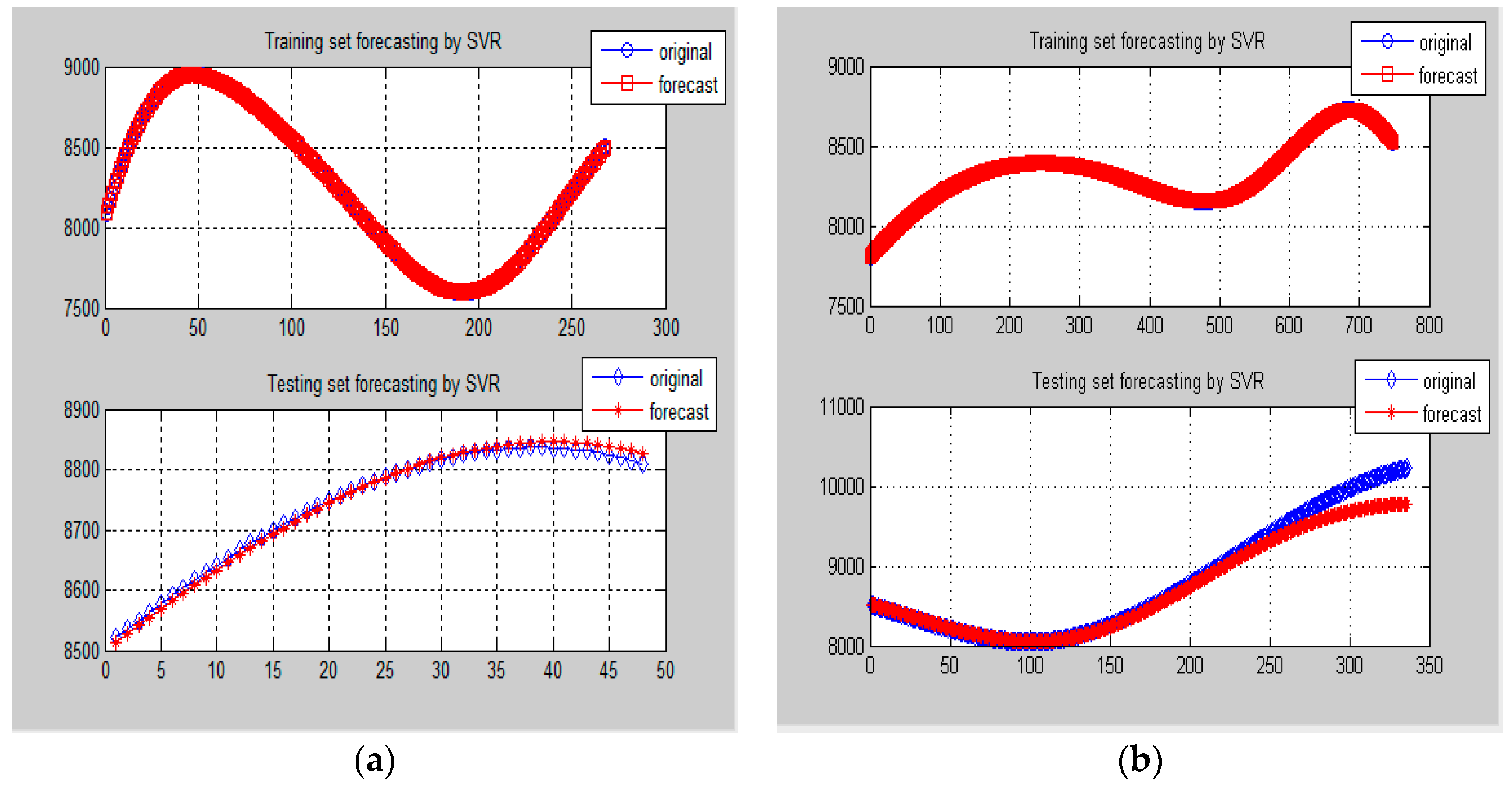
Figure 9.
The hour based original data, Data-I, Data-II (Example 2). (a) Small data size (1–14 January 2015); (b) Large data size (1 January–15 February 2015).
Figure 9.
The hour based original data, Data-I, Data-II (Example 2). (a) Small data size (1–14 January 2015); (b) Large data size (1 January–15 February 2015).

Figure 10.
The decomposed different items for the small data size (Example 2). (a) IMF (intrinsic modulo function) 1; (b) IMF 2; (c) IMF 3; (d) IMF 4; (e) IMF 5; (f) IMF 6; (g) IMF 7; (h) IMF 8; (i) residuals.
Figure 10.
The decomposed different items for the small data size (Example 2). (a) IMF (intrinsic modulo function) 1; (b) IMF 2; (c) IMF 3; (d) IMF 4; (e) IMF 5; (f) IMF 6; (g) IMF 7; (h) IMF 8; (i) residuals.
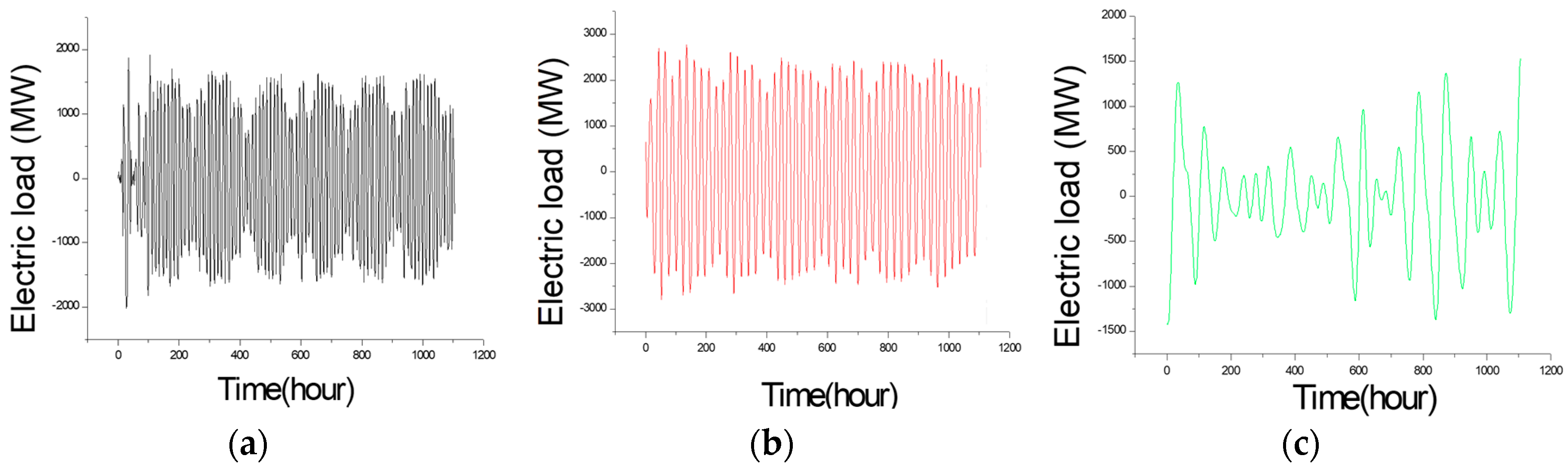

Figure 11.
Comparison of forecasting results by SVR-PSO model for Data-I (Example 2). (a) One-day ahead forecasting from 13 to 14 January 2015; (b) One-week ahead forecasting from 2 to 15 February 2015.
Figure 11.
Comparison of forecasting results by SVR-PSO model for Data-I (Example 2). (a) One-day ahead forecasting from 13 to 14 January 2015; (b) One-week ahead forecasting from 2 to 15 February 2015.

Figure 12.
Comparison of forecasting results by SVR-GA model for Data-II (Example 2). (a) One-day ahead forecasting from 13 to 14 January 2015; (b) One-week ahead forecasting from 2 to 15 February 2015.
Figure 12.
Comparison of forecasting results by SVR-GA model for Data-II (Example 2). (a) One-day ahead forecasting from 13 to 14 January 2015; (b) One-week ahead forecasting from 2 to 15 February 2015.

Figure 13.
Forecasting performances comparisons (Example 1). (a) One-day ahead forecasting on 8 May 2007; (b) One-week ahead forecasting from 18 to 24 May 2007.
Figure 13.
Forecasting performances comparisons (Example 1). (a) One-day ahead forecasting on 8 May 2007; (b) One-week ahead forecasting from 18 to 24 May 2007.

Figure 14.
Forecasting performance comparisons (Example 2). (a) One-day ahead forecasting from 13 to 14 January 2015; (b) One-week ahead forecasting from 2 to 15 February 2015.
Figure 14.
Forecasting performance comparisons (Example 2). (a) One-day ahead forecasting from 13 to 14 January 2015; (b) One-week ahead forecasting from 2 to 15 February 2015.

Figure 15.
The local enlargement (peak) comparisons (Example 2). (a) One-day ahead forecasting from 13 to 14 January 2015; (b) One-week ahead forecasting from 2 to15 February 2015.
Figure 15.
The local enlargement (peak) comparisons (Example 2). (a) One-day ahead forecasting from 13 to 14 January 2015; (b) One-week ahead forecasting from 2 to15 February 2015.

Table 1.
The parameters settings of SVR-PSO model for original data and Data-I (Examples 1 and 2).
| Data Types | Number of Particle | Length of Particle | Constant q1 | Constant q2 | Maximum of Iteration | Cmin | Cmax | σmin | σmax |
|---|---|---|---|---|---|---|---|---|---|
| Original data | 30 | 3 | 2 | 2 | 300 | 0 | 200 | 0 | 200 |
| Small data size | 20 | 3 | 2 | 2 | 50 | 0 | 200 | 0 | 200 |
| Large data size | 5 | 3 | 2 | 2 | 20 | 0 | 200 | 0 | 200 |
Table 2.
The SVR-PSO’s parameters for Data-I (Example 1).
| Data Size | σ | C | ε | Testing MAPE | Testing RMSE |
|---|---|---|---|---|---|
| Samall data size | 0.15 | 91 | 0.0025 | 9.14 | 101.76 |
| Large data size | 0.20 | 99 | 0.0012 | 4.15 | 102.57 |
Table 3.
The parameters settings of SVR-GA model for original data and Data-II (Examples 1 and 2).
| Data Types | Population Size | Mutation Rate | Crossover Rate | Maximum of Generation | Cmin | Cmax | σmin | σmax |
|---|---|---|---|---|---|---|---|---|
| Original data | 100 | 0.05 | 0.8 | 200 | 0 | 100 | 0 | 1000 |
| Small data size | 100 | 0.05 | 0.8 | 200 | 0 | 100 | 0 | 1000 |
| Large data size | 100 | 0.05 | 0.8 | 200 | 0 | 100 | 0 | 1000 |
Table 4.
The SVR-GA’s parameters for Data-II (Example 1).
| Data Size | σ | C | ε | Testing MAPE | Testing RMSE |
|---|---|---|---|---|---|
| Samall data size | 0.15 | 90 | 0.0022 | 8.70 | 69.79 |
| Large data size | 0.20 | 95 | 0.0015 | 3.83 | 98.79 |
Table 5.
The SVR-PSO’s parameters for Data-I (Example 2).
| Data Size | σ | C | ε | Testing MAPE | Testing RMSE |
|---|---|---|---|---|---|
| Small data size | 0.12 | 80 | 0.0021 | 7.21 | 110.04 |
| Large data size | 0.24 | 89 | 0.0012 | 4.70 | 115.63 |
Table 6.
The SVR-GA’s parameters for Data-II (Example 2).
| Data Size | σ | C | ε | Testing MAPE | Testing RMSE |
|---|---|---|---|---|---|
| Samall data size | 0.15 | 90 | 0.0023 | 7.02 | 82.11 |
| Large data size | 0.22 | 98 | 0.0012 | 4.41 | 96.83 |
Table 7.
Forecasting performances of competitive models for both small and large data sizes (Example 1).
Table 7.
Forecasting performances of competitive models for both small and large data sizes (Example 1).
| Models | MAPE | RMSE | MAE | AIC | BIC |
|---|---|---|---|---|---|
| Small Data Size | |||||
| Original SVR | 11.70 | 145.87 | 10.92 | −79.76 | −68.71 |
| SVR-PSO | 11.41 | 145.69 | 10.67 | −79.94 | −68.89 |
| SVR-GA | 13.52 | 150.38 | 11.88 | −75.31 | −64.26 |
| AFCM [35] | 9.95 | 125.32 | 9.26 | −101.92 | −90.87 |
| EMD-PSO-GA-SVR | 9.09 | 123.38 | 9.19 | −104.19 | −93.14 |
| Large Data Size | |||||
| Original SVR | 12.88 | 181.62 | 12.05 | −823.32 | −812.27 |
| SVR-PSO | 13.50 | 271.43 | 13.07 | −630.68 | −619.63 |
| SVR-GA | 14.31 | 183.57 | 15.31 | −818.20 | −807.15 |
| AFCM [35] | 11.10 | 158.75 | 10.44 | −887.85 | −876.80 |
| EMD-PSO-GA-SVR | 3.92 | 142.41 | 9.04 | −939.93 | −928.88 |
Table 8.
Forecasting performances of competitive models for both small and large data sizes (Example 2).
Table 8.
Forecasting performances of competitive models for both small and large data sizes (Example 2).
| Models | MAPE | RMSE | MAE | AIC | BIC |
|---|---|---|---|---|---|
| Small Data Size | |||||
| Original SVR | 19.43 | 220.92 | 22.33 | −19.19 | −8.14 |
| SVR-PSO | 18.76 | 200.53 | 21.19 | −33.32 | −22.27 |
| SVR-GA | 17.98 | 201.74 | 22.58 | −32.44 | −21.39 |
| AFCM [35] | 14.31 | 158.11 | 17.44 | −68.00 | −56.95 |
| EMD-PSO-GA-SVR | 7.15 | 137.30 | 14.44 | −88.59 | −77.54 |
| Large Data Size | |||||
| Original SVR | 33. 72 | 321.44 | 32.05 | −549.60 | −538.55 |
| SVR-PSO | 37.51 | 300.32 | 31.39 | −582.18 | −571.13 |
| SVR-GA | 34.20 | 298.11 | 26.31 | −585.73 | −574.68 |
| AFCM [35] | 11.29 | 289.21 | 20.76 | −600.26 | −589.21 |
| EMD-PSO-GA-SVR | 4.63 | 150.82 | 15.20 | −912.42 | −901.37 |
Table 9.
Wilcoxon signed-rank test.
| Examples | Compared Models | Wilcoxon Signed-Rank Test α = 0.05; W = 6 |
|---|---|---|
| Example 1 | EMD-PSO-GA-SVR vs. Original SVR | 3 a |
| EMD-PSO-GA-SVR vs. SVR-PSO | 2 a | |
| EMD-PSO-GA-SVR vs. SVR-GA | 2 a | |
| EMD-PSO-GA-SVR vs. AFCM | 2 a | |
| Example 2 | EMD-PSO-GA-SVR vs. Original SVR | 2 a |
| EMD-PSO-GA-SVR vs. SVR-PSO | 2 a | |
| EMD-PSO-GA-SVR vs. SVR-GA | 2 a | |
| EMD-PSO-GA-SVR vs. AFCM | 2 a |
a Denotes that the proposed EMD-PSO-GA-SVR model is significantly superior to other competitive models.
© 2017 by the authors. Licensee MDPI, Basel, Switzerland. This article is an open access article distributed under the terms and conditions of the Creative Commons Attribution (CC BY) license (http://creativecommons.org/licenses/by/4.0/).
Share and Cite
MDPI and ACS Style
Fan, G.-F.; Peng, L.-L.; Zhao, X.; Hong, W.-C. Applications of Hybrid EMD with PSO and GA for an SVR-Based Load Forecasting Model. Energies 2017, 10, 1713. https://doi.org/10.3390/en10111713
AMA Style
Fan G-F, Peng L-L, Zhao X, Hong W-C. Applications of Hybrid EMD with PSO and GA for an SVR-Based Load Forecasting Model. Energies. 2017; 10(11):1713. https://doi.org/10.3390/en10111713
Chicago/Turabian StyleFan, Guo-Feng, Li-Ling Peng, Xiangjun Zhao, and Wei-Chiang Hong. 2017. "Applications of Hybrid EMD with PSO and GA for an SVR-Based Load Forecasting Model" Energies 10, no. 11: 1713. https://doi.org/10.3390/en10111713
Note that from the first issue of 2016, this journal uses article numbers instead of page numbers. See further details here.