Aggregation Methods for Modelling Hydropower and Its Implications for a Highly Decarbonised Energy System in Europe

Abstract

Given the pursuit of long-term decarbonisation targets, future power systems face the task of integrating the renewable power and providing flexible backup production capacity. Due to its general ability to be dispatched, hydropower offers unique features and a backup production option not to be neglected, especially when taking the flexibility potential of multireservoir systems into account. Adequate hydropower representations are a necessity when analysing future power markets and aggregation methods are crucial for overcoming computational challenges. However, a major issue is that the aggregation must not be a too flexible representation. In a first step, a novel equivalent hydro system model implementation including a possibility to integrate pumping capacity and appropriate handling of multiple water paths (hydraulic coupling) by making use of an ex-ante optimisation is proposed. In a second step, a clustered equivalent hydro system model implementation employing k-means clustering is presented. A comparison of both aggregation approaches against the detailed reference system shows that both aggregated model variants yield significant reductions in computation time while keeping an adequate level of accuracy for a highly decarbonised power system scenario in Europe. The aggregation methods can easily be applied in different model types and may also be helpful in the stochastic case.

1. Introduction

1.1. Role of Hydropower in Future Power Systems

Pursuing its long-term decarbonisation targets, Europe’s power systems will be increasingly shaped by renewable power generation from wind power and solar photovoltaics. Given the fluctuating nature of these generation technologies, the future power system faces the task of integrating the renewable power and providing flexible backup production capacity from conventional power sources.

Although hydroelectric resources are mostly tapped into and its generation capacity is not expected to experience large-scale expansions, it can be assumed that renewable generation from hydropower is going to persist and continue playing an important role in future power systems. Due to its general ability to be dispatched, hydropower offers unique features and a backup production option not to be neglected. While still being subject to weather-dependent phenomena, i.e., variations of natural inflow, hydropower systems with storage reservoirs can provide valuable short- to long-term system flexibility, particularly cascaded multireservoir hydro valleys. Additionally, the availability of pumping capacity in hydropower systems adds a further degree of operational freedom. Hence, it is essential to adequately address hydropower when analysing future power systems.

1.2. Implications for Power Market Models

In the context of power systems, crucial tasks such as price forecasting, operation planning, analysis of the security of supply and investment analysis require sophisticated hydro-thermal market simulation and optimisation models. Depending on the area and focus of the analysis, a large number of hydro plants and reservoirs can severely amplify the market model complexity, e.g., in the Nordic and Alpine regions in Europe. This is particularly the case for cascaded multireservoir systems which are subject to uncertain natural inflows and require simultaneous operational decisions for each reservoir in the system [1].

As a consequence, market models with an ample geographical scope mostly rely on aggregated representations of the relevant hydro systems. Since the European power market will see stronger coupling and experience larger quantities of non-dispatchable renewable generation from wind and solar, these market modelling challenges are only becoming more difficult. At the same time, however, capturing short-, medium-, and long-term dynamics, including those of hydropower systems, is essential when analysing the need for future system flexibility and its implications.

1.3. Aggregation Methods in Power Market Models

Facing the challenge of solving high-dimensional optimisation problems, aggregation methods which develop auxiliary models with reduced complexity, but, at the same time, providing good approximations of the original problem can be instrumental [2]. There are various reasons for using aggregation approaches in operations research, as pointed out in [3]. In this context, a lack of reliable micro-level data for building a detailed model, the possibility of obtaining results at different levels of detail, as well as reducing the inherent computational burden are the most relevant among them.

A major challenge is that the aggregation must not be a too flexible representation in the power market model. For instance, a lump sum hydropower formulation as was used in [4] can yield flexibility overestimations of the power system, which can be problematic when analysing grid or generation capacity expansion planning problems.

1.4. Previous Work on Hydro System Aggregation

Ultimately, the challenges outlined above amount to the general and well known problem of determining the optimum operation of a multireservoir hydro system, particularly long-term operation [5]. As numerous computer simulations models were developed and applied within many river basins over the last decades, e.g., [6,7], the task of making rational operational decisions for reservoir systems has been extensively studied. Nowadays, various solution strategies for customised reservoir system optimisation problems exist and are being further developed [8].

Of particular interest is the previous work that has been carried out to identify seasonal operation strategies for multireservoir systems by using state aggregation approaches [9]. More specifically, the concept of a composite or equivalent reservoir model for the hydro system becomes necessary because a complexity reduction of the model is inevitable. By aggregating a hydro system with multiple interconnected hydraulic reservoirs into a single equivalent reservoir, this method tries to construct a suitable mathematical model producing the same water outputs as would be produced by the original hydro system. According to [10], this idea and its underlying principle of simplifying the complex multireservoir hydropower systems originates from [11]. In a similar manner and with a focus on the total hydro generation rather than the allocation among the various hydro plants, a composite model is put forward representing the main characteristics and capabilities of the original hydro system in [12].

Dynamic programming has been widely used to solve operational optimisation problems of hydropower systems [2]. As one important drawback, these programs can suffer from the curse of dimensionality, which is particularly true for systems with multiple interconnected hydraulic reservoirs [13]. To overcome the dimensionality problem in dynamic programming, the aggregation of all reservoirs into an equivalent reservoir (state aggregation) was, according to [8], first used by [14]. After obtaining the optimised operation schedule of the aggregated reservoir it is translated into individual policies for each reservoir bound by the aggregate solution.

In [15], this concept is extended to stochastic dynamic programming by using an equivalent reservoir representation of a large-scale hydropower system with stochastic inflows. Using a space-time aggregation-disaggregation procedure, this approach has, for instance, been applied to the real-time operation of a four-reservoir system in Venezuela by [16].

On a more general note, [10] outlines three guiding principles of disaggregation-aggregation for identifying the optimal operation of a multireservoir system. To be more specific, the resulting sub-problems of these principles have been summarised by [17] as:

• formulating a single equivalent hydro system model representing the multireservoir system,
• determining the optimal operation of such a single equivalent hydro system model,
• disaggregating such optimal operation into the operation of the original multireservoir system.

Regarding the third sub-problem of disaggregation, reference [13] presented a non-linear disaggregation technique for the operation of multireservoir systems incorporating neural networks and compared it to a principal component analysis technique. In [18], a hierarchical procedure based marginal values is used to disaggregate the hydropower production among the aggregated rivers of a 26 reservoir system. With that in mind, the disaggregation task is of lower priority in this context, particularly when long-term analyses are carried out, see Section 1.2. This is because achieving computationally efficient aggregations to reasonably capture their flexibility contribution is of greater importance than the scheduling decisions of individual plants.

More recently, research on extending the equivalent hydro system model has examined the possible gains of using a model with not one but two stations linked together to represent a larger system [19], and of incorporating hydraulically coupled sub-systems [20]. Using different hydro reservoir characteristics, such as the duration to empty the reservoir and the possibility of pumping, when building the equivalent hydro system models is referred to in [21]. Here, three independent aggregated reservoirs to calculate Bellman functions [22] for hydraulic reservoirs. Based on a serially linked two-stage reservoir system in [17], an aggregation/disaggregation technique is discussed in [2] to mitigate dimensionality problems in analysing multireservoir systems by means of a hypothetical composite reservoir.

An alternative method based on the stochastic dual dynamic programming approach (SDDP) was developed in [23], which overcomes the dimensionality problem so that large-scale systems can be investigated [24].

Contrary to the bottom-up approaches mentioned above, two top-down approaches for representing European hydropower in power system models have been studied in [25,26].

In summary, while some research has been carried out on aggregated models for multireservoir systems, no studies have been found which evaluate different levels of aggregation on the European power system level. As a notable exception, [9] examines the influence of the involved simplification procedures on the results obtained from equivalent reservoir models of the São Francisco River Hydroelectric System in Brazil by comparing them to those obtained from an operational optimisation model considering the individual reservoir characteristics. In [27], two power market models, one simplified and one detailed, are used to model possible balancing responses of Norwegian hydropower to a wind-driven exchange pattern for various amounts of exchange capacity.

What remains unclear is how a bottom-up aggregation approach based on detailed hydro systems, i.e., reservoir, plant, and interconnection data, can be adequately built and used to represent the entire hydropower complex in Europe, and what implications these aggregation measures can have on the results from power market analysis models.

Of equal importance is the fact that existing aggregation techniques are not well adapted to new challenges introduced by the system changes mentioned in Section 1.1. A larger share of new renewable energy, stronger coupling of market areas within Europe, and the potential for large-scale pumped storage enhance the weaknesses of the existing aggregation methods. The operation of pumped storage plants, often as part of cascaded multireservoir systems, has to be properly addressed in aggregated hydro system model formulations. For instance, pump operations in the aggregated EMPS model [7] rely on rule-based decisions resulting in potentially inadequate pumping strategies.

As a result of the above, computationally efficient aggregation methods improving the model properties in general and specifically with regard to the new market and system challenges in decarbonised energy systems are essential and need to be investigated.

1.5. Main Contributions

The main contributions of this article can be summarised as:

• bottom-up data base for hydropower systems across Europe comprising detailed hydro plant and reservoir information,
• natural inflow model relying only on basic prerequisite hydro reservoir data,
• novel equivalent hydro system model implementation including a possibility to integrate pumping capacity and adequate handling of multiple water paths (hydraulic coupling) by making use of an ex-ante optimisation,
• novel clustered equivalent hydro system model implementation employing k-means clustering,
• comparison and evaluation of both the equivalent and clustered equivalent hydro system model formulations with the detailed reference hydro system for a highly decarbonised power system scenario in Europe, in which flexibility is a key aspect.

In the remaining part of this article, Section 2 describes the bottom-up hydro reservoir and plant data base, and explains the natural inflow model. Serving as the reference representation throughout this analysis, the detailed hydro system model is presented in Section 3. Section 4 introduces the first level of aggregation by presenting the equivalent hydro system model. Employing a clustering technique, Section 5 proposes an additional level of aggregation to reduce the computational burden even further. In Section 6, both aggregation approaches are tested and evaluated against the detailed reference model in a case study. Section 7 discusses the obtained results and Section 8 concludes the study.

2. Hydropower Data Base and Inflow Model

2.1. Hydro Reservoir and Plant Data

Through a process of collecting and combining publicly available information, an extensive data base of all in all 734 hydro systems across Europe’s major market areas has been established. The underlying sources of information range from a large number of published reports, e.g., [28,29,30], spreadsheets, e.g., [31,32], and interactive maps, e.g., [33,34,35], on a federal and regional level, to individual operator’s hydro plant information provided on websites, e.g., [36,37]. Note that the data set includes existing hydro systems as well as substantiated future hydropower projects.

Regarding hydro plants, the data base comprises essential structural data, i.e., power rating, turbine type, (net) head, historical or expected average annual energy production, as well as information about market area participation. The latter information is particularly relevant for cross-border power plants participating in more than one market area, or plants located in one market area but generating or consuming their power in another. The hydro reservoir data includes active reservoir volume, reservoir stage, as well as spillage target information. Information about the interconnection of hydro reservoirs and plants was determined for each system and implemented in a flexible object-oriented MATLAB, R2016a (MathWorks, Natick, MA, USA) environment.

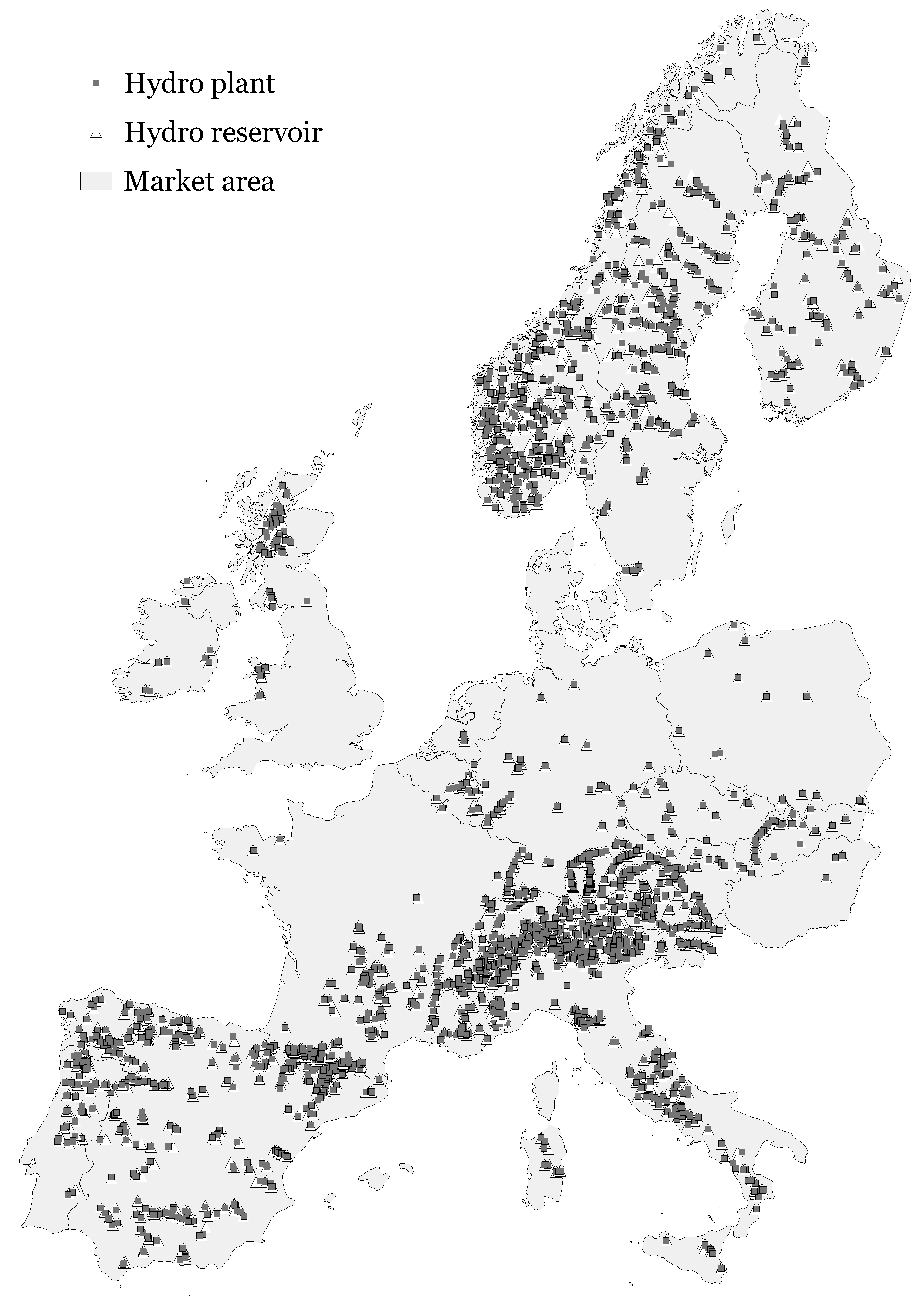
For all hydro plants and reservoirs, geographic locations have been gathered. Figure 1 illustrates their spatial coverage across the considered market areas in Europe. From the map, it can be seen that the majority of hydro systems in Europe is located in Scandinavia, the Alps, and the Iberian Peninsula.

In most market areas, a large number of hydropower plants exists with only a small turbine capacity, frequently below 10 MW. Because the available information for these systems is sparse, at best, the small hydropower plants are aggregated in each market area and considered as a generic conventional hydro storage system, or a generic run-of-the-river hydro system, or both. Exceptions are of course small hydro plants which already belong to a bigger hydro system.

2.2. Hydro System Classification

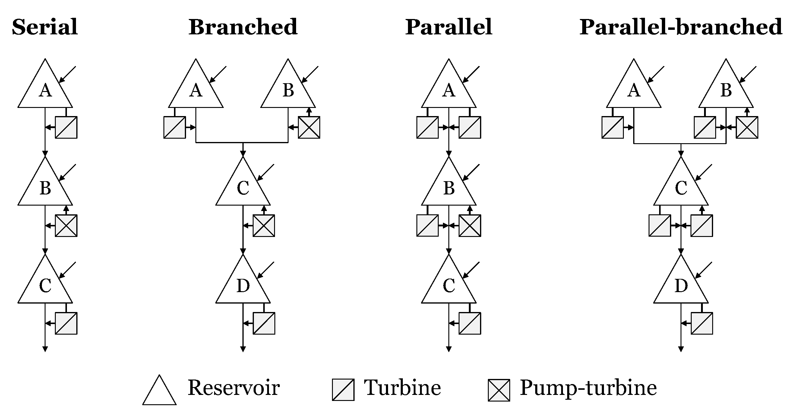
It is important to acknowledge the structural differences in hydro systems since they can have a significant impact on the applicability of aggregation techniques. More specifically, the way of how cascaded reservoirs are interconnected, as well as the presence of pumping capacities between those reservoirs, make the application of aggregation methods more complex and, therefore, cannot be ignored. To better understand and distinguish the decisive features, a classification of hydro systems is presented in Figure 2.

Beside one-stage hydro systems with only one separate upper reservoir, multistage reservoir systems are categorised in serial, branched, parallel, and parallel-branched systems in this context. Note that all system classifications can contain turbines, pumped hydro turbines, or pumps in any combination.

Serial systems commonly follow natural river beds to end up in big inland water bodies or estuaries. These systems mainly differ in the composition of reservoir capacities and natural inflow volumes.

Branched systems exist if multiple reservoirs are connected to one reservoir. Typically, these system configurations occur in mountainous regions where snow and water accumulate in elevated catchment areas and confluence during the descent. Less frequently, branched systems can split up in the intermediate or final stages.

Parallel systems imply a parallel interconnection of hydro reservoirs and plants. In many cases, large reservoirs exhibit several connected hydro plants enabling the water to take different downstream paths. The parallel paths are not necessarily limited to a step of one stage and can exhibit different lengths, i.e., reservoir stages. Regarding the aggregation approach, capturing these opportunities poses a significant challenge, see also [20].

Parallel-branched systems are the most complex systems as they show branched and parallel characteristics at the same time.

2.3. Natural Inflow Model

As with structural parameters characterising hydro plants and reservoirs in general, public availability of reservoir inflow data is particularly difficult. It often is the operator’s proprietary information or the data is not centrally gathered and managed, as is especially the case with smaller hydropower systems. Even if in some cases reservoir inflow data can be acquired, its temporal resolution or the necessary time span might be insufficient.

For the purpose of this study, a generic approach needs to be employed yielding natural inflow profiles of each single hydro reservoir in the considered market areas. To be more specific, the main idea is to use historical runoff data in order to create reservoir-specific normalised inflow profiles which are then adjusted to individual hydro plant production data.

The historical runoff data is based on the global atmospheric reanalysis ERA-Interim produced by the European Centre for Medium-Range Weather Forecasts (ECMWF) [38]. It covers the period from 1979 onward and continues being extended forward, generating gridded data of three-hourly surface parameters among others (for a detailed description of the ERA-Interim model, data and assimilation method see [39]).

ERA-Interim’s runoff parameter is measured in m of water and can be obtained on a 0.125${}^{\circ }$ × 0.125${}^{\circ }$ latitude/longitude grid. The availability of spatially distributed data allows the creation of site-specific normalised runoff profiles matching the reservoir’s surrounding conditions. Based on the reservoir’s geographic location, an initial cubic spatial interpolation of the available runoff data points is carried out. This is followed by a cubic temporal interpolation to obtain hourly data from the three-hourly data set for each considered historical climate reference years (2000–2013 in this case).

After determining a hydro reservoir’s normalised runoff profiles for the given set of meteorological reference years, the second crucial step involves adjusting these to the historical or expected (new plants) production data for all hydro plants connected to this reservoir. In the detailed hydro representation, the resulting inflow profile $q_{hjt}^{\mathrm{N}}$ for a given meteorological reference year is to resemble the corresponding amount of water flowing into the reservoir (${\mathrm{hm}}^3/\mathrm{h}$), which can be used for hydroelectric production in that year. A hydro plant’s detailed production data is rarely accessible for a full range of historical years, but an average annual energy generation figure can often be found or derived from published data. To determine the annual inflow variations, these average annual energy generation values are combined with the variations gathered from ERA-Interim’s total annual runoff data.

Since the natural inflow volumes are determined on an individual hydro reservoir basis, this approach can lead to over-estimations in a multireservoir system. For instance, if an upstream reservoir receives more water than the subsequent reservoir stage needs to produce its electricity, only a share of the water can remain in the considered hydro system. Therefore, a system conservation coefficient ${\kappa }_{hj}\in [0,1]$ is determined based on the annual amounts of inflowing water ($q_{hit}^{\mathrm{N}}$), indicating this share.

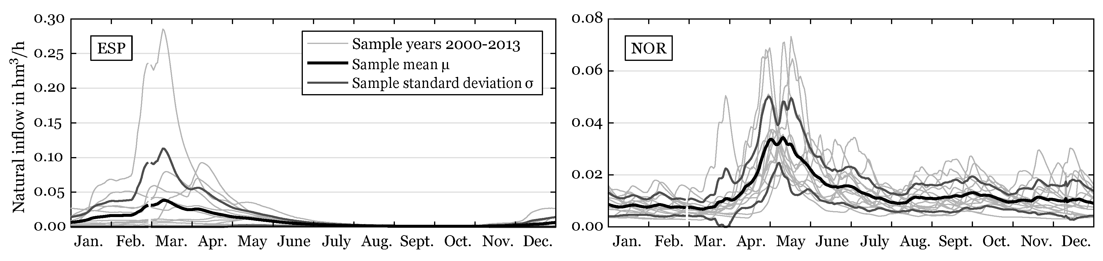
In Figure 3, the resulting natural inflow profiles for a hydro reservoir in Spain and Norway are shown for 14 meteorological reference years.

3. Detailed Hydro System Model

3.1. Hydraulic Coupling

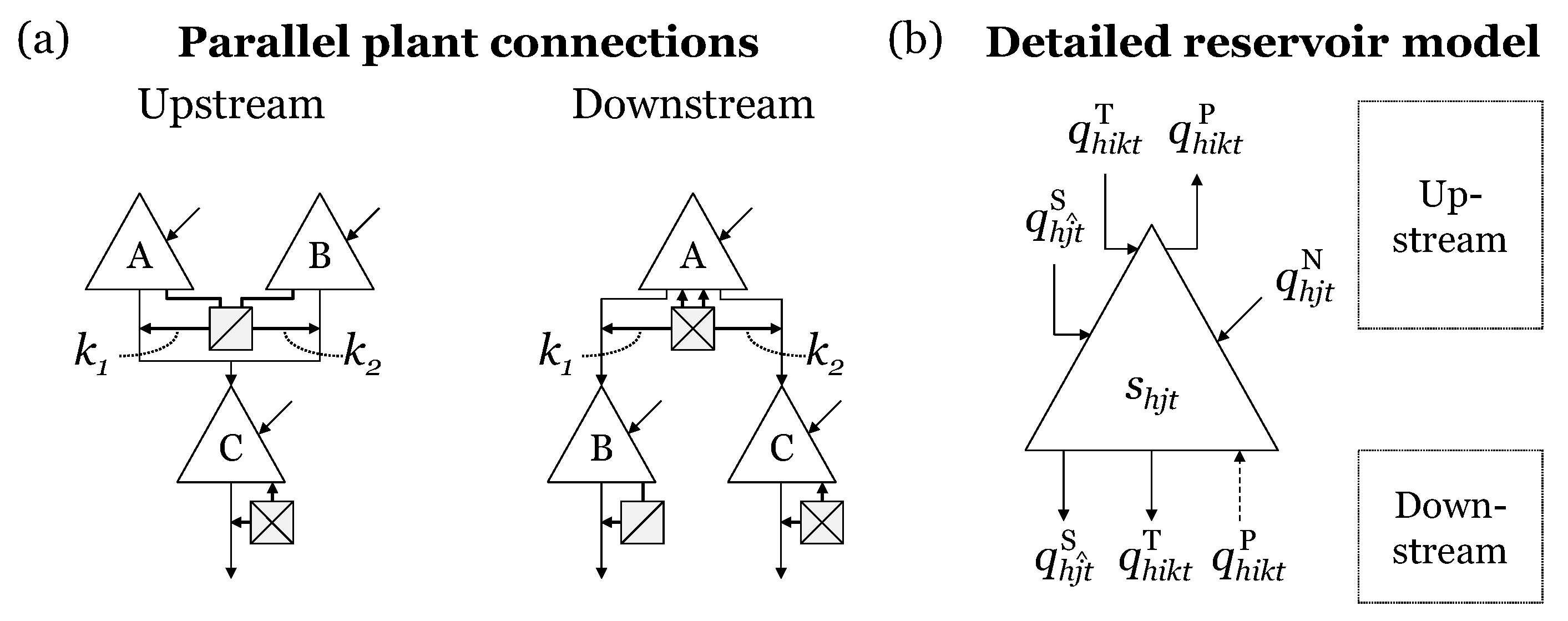
Before introducing the detailed hydro system model it is important to recognise the possibility of hydraulically coupled reservoir configurations. If two or more reservoirs are either coupled through a tunnel or channel, or connected to a common up- or downstream hydro plant (parallel plant connections), the water flow distribution is an optimisation result and needs to be treated as a decision variable, see Figure 4a.

3.2. Detailed Model Formulation

Besides the natural inflow, the detailed reservoir has many potential up- and downstream in- and outflow connections due to turbine, pump, and spillage links which need to be taken into account, see Figure 4b.

Based on the principle of continuity, Equation (1) ensures the balance of each hydro reservoir’s active storage level

$$\begin{array}{c}{s}_{hj{t}^{\prime }}=s_{hjt}+q_{hjt}^{\mathrm{N}}+{\displaystyle \sum _i^{I_{hj}^{\mathrm{US}}}}{\displaystyle \sum _k^{K_{hij}}}{q}_{hikt}^{\mathrm{T}}·{\kappa }_{hj}-{\displaystyle \sum _i^{I_{hj}^{\mathrm{DS}}}}{\displaystyle \sum _k^{K_{hij}}}{q}_{hikt}^{\mathrm{T}}-{\displaystyle \sum _i^{I_{hj}^{\mathrm{US}}}}{\displaystyle \sum _k^{K_{hij}}}{q}_{hikt}^{\mathrm{P}}+{\displaystyle \sum _i^{I_{hj}^{\mathrm{DS}}}}{\displaystyle \sum _k^{K_{hij}}}{q}_{hikt}^{\mathrm{P}}+{\displaystyle \sum _{\widehat{j}}^{J_{hj}^{\mathrm{US}}}}{q}_{h\widehat{j}jt}^{\mathrm{S}}·{\kappa }_{hj}-{\displaystyle \sum _{\widehat{j}}^{J_{hj}^{\mathrm{DS}}}}{q}_{hj\widehat{j}t}^{\mathrm{S}}\forall h,j,t\end{array}$$

(1)

where $I_{hj}^{\mathrm{US}}$ and $I_{hj}^{\mathrm{DS}}$ denote the subsets of all upstream (US) and downstream (DS) hydro plants directly connected to hydro reservoir j of hydro system h, respectively. Similarly, the subsets $J_{hj}^{\mathrm{US}}$ and $J_{hj}^{\mathrm{DS}}$ contain all upstream and downstream hydro reservoirs directly connected through spillage to hydro reservoir j of hydro system h, respectively. Note that evaporation is not considered here.

In all time steps, the reservoir storage belongs to the set of admissible storage volume, which is defined by Equation (2).

$$s_{hj}^{\min }\le s_{hjt}\le s_{hj}^{\max }\forall h,j,t$$

(2)

For the purpose of this study, the hydro system operation is carried out for an annual cycle, i.e., a full consecutive year in hourly resolution. Hence, Equation (3) ensures that the active storage volume complies with initial and final values which do not necessarily have to be equal.

$$s_{hj{t}_1}=s_{hj}^{\mathrm{initial}}{s}_{hj{t}_{\left|T\right|+1}}\ge s_{hj}^{\mathrm{final}}\forall h,j$$

(3)

Moreover, the amount of spilled water cannot be negative, implying that

$$0\le q_{hj\widehat{j}t}^{\mathrm{S}}\widehat{j}\in J_{hj}^{\mathrm{DS}}\forall h,j,t$$

(4)

As denoted in Equations (5) and (6), the turbine and pump energy conversion coefficients describe a hydro plant’s out- and input behaviour in a very simple linear form with a constant head:

$${\pi }_{hik}^{\mathrm{T}}=\frac{1}{3600}·\gamma ·g·h_{hik}^{\mathrm{T}}·{\eta }_{hi}^{\mathrm{T}}\forall h,i,k$$

(5)

$${\pi }_{hik}^{\mathrm{P}}=\frac{1}{3600}·\gamma ·g·h_{hik}^{\mathrm{P}}·\frac{1}{{\eta }_{hi}^{\mathrm{P}}}\forall h,i,k$$

(6)

Whereas in reality the efficiency of the plant will depend on its discharge and varying head, thereby rendering the hydroelectric production function non-linear, a constant energy equivalent coefficient for both turbine and pump units is assumed in this context. This implies that the hydroelectric generation and consumption in Equations (7) and (8) are only proportional to the water discharge and intake, respectively.

$$x_{hit}^{\mathrm{T}}=\sum _k^{K_{hi}}{\pi }_{hik}^{\mathrm{T}}·q_{hikt}^{\mathrm{T}}\forall h,i,t$$

(7)

$$x_{hit}^{\mathrm{P}}=\sum _k^{K_{hi}}{\pi }_{hik}^{\mathrm{P}}·q_{hikt}^{\mathrm{P}}\forall h,i,t$$

(8)

In view of the data availability and the purpose of this model, the simplification above is deemed reasonable. Importantly, it is then possible to quantify an amount of water in energy units (MWh) [40], which is vital for the aggregation approach [12].

In Equations (9) and (10), the constraints limit the hydro plant’s turbine generation and pump consumption of electrical energy.

$$x_{hi}^{\mathrm{T},\min }\le x_{hit}^{\mathrm{T}}\le x_{hi}^{\mathrm{T},\max }\forall h,i,t$$

(9)

$$x_{hi}^{\mathrm{P},\min }\le x_{hit}^{\mathrm{P}}\le x_{hi}^{\mathrm{P},\max }\forall h,i,t$$

(10)

4. Equivalent Hydro System Model

4.1. Assumptions

Before introducing the aggregation approach of a multireservoir hydroelectric system, it is mandatory to highlight the underlying assumptions which, in accordance with [15], are:

• The amount of electrical energy generated or consumed by any power plant i in period t is a constant times the discharge or intake, see Equations (7) and (8).
• The optimal operating policy of hydro system h is such that spillage will not occur in period t or will occur at every reservoir j of the hydro system h, and a shortage of water will not occur in period t or will occur in every reservoir j of the river.

4.2. Conversion Coefficients

Based on the assumptions above, an equivalent one-dam representation of each hydro system h can be built. To aggregate the reservoirs of a hydro system, it suffices to convert the water stored at each plant into its at-site and downstream generating capability and to sum over all plants. As this concept has been well established, e.g., in [12,15,18], the following part describes the conversion coefficients with a crucial level of implementational detail becoming necessary when not only dealing with serially linked hydro systems.

Particular attention has to be paid if the water being released from reservoir j can take more than one downstream path, either through different hydro plants i or different parallel plant connections k of one hydro plant, see Figure 2 and Figure 4.

It is suggested in [18] to assume that the water always takes the downstream path which maximises the potential energy. However, this paradigm can lead to significant overestimations, e.g., of the energy inflow, while building the equivalent model. Given a reservoir with two downstream paths, one exhibiting a higher conversion coefficient than the other, but only a small discharge capacity compared to the second one, the tendency to overestimate by always taking the first path becomes obvious.

Moreover, unavoidable spillage of single hydro reservoirs appearing in the detailed model must be factored in, since this effect will presumably be neglected by the equivalent hydro system model.

Therefore, a novel way of determining the conversion coefficients at each reservoir with multiple paths is required, especially if no detailed historical production data is available. To that end, the weighted average turbine conversion coefficient, measured in $\mathrm{MWh}/{\mathrm{hm}}^3$, is introduced for hydro reservoir j of hydro system h. It can be denoted as

$${\pi }_{hj}^{\mathrm{T}}=\sum _i^{I_{hj}^{\mathrm{DS}}}\sum _k^{K_{hij}}{\varphi }_{hik}^{\mathrm{T}}·\left({\pi }_{hik}^{\mathrm{T}}+{\pi }_{h{\widehat{j}}_{hik}}^{\mathrm{T}}·{\kappa }_{h{\widehat{j}}_{hik}}\right)\forall h,j$$

(11)

where ${\widehat{j}}_{hik}$ refers to the hydro reservoir directly connected to downstream path k of hydro plant i from hydro reservoir j, and ${\varphi }_{hik}^{\mathrm{T}}$ is the downstream path distribution coefficient which is represented by a constant weight, indicating how much water will be discharged through the corresponding path.

Thus, the weights of all potential downstream paths of hydro reservoir j in hydro system h must sum up to one:

$$\sum _i^{I_{hj}^{\mathrm{DS}}}\sum _k^{K_{hij}}{\varphi }_{hik}^{\mathrm{T}}=1\forall h,j$$

(12)

Note the recursive nature of Equation (11) for which the recursive term ${\pi }_{h{\widehat{j}}_{hik}}^{\mathrm{T}}$ diminishes in every last stage of the recursion tree, or, in this context, for every final reservoir at the end of a downstream path in hydro system h. Given the purpose of the system conservation coefficient in Equation (1), ${\kappa }_{hj}$ has to be taken into account when determining the average turbine conversion coefficient as well.

With that in mind, it has remained unclear how the downstream path distribution coefficient can be determined. In Equation (13), it is defined as the ratio of the accumulated amount of water being discharged during all considered time steps through one downstream path versus all possible paths leaving hydro reservoir j:

$${\varphi }_{hik}^{\mathrm{T}}=\frac{{\sum }_t^T{q}_{hikt}^{\mathrm{T}*}}{{\sum }_i^{I_{hj}^{\mathrm{DS}}}{\sum }_k^{K_{hij}}{\sum }_t^T{q}_{hikt}^{\mathrm{T}*}}\forall h,i,k$$

(13)

Here $q_{hikt}^{\mathrm{T}*}$ represents a known turbine discharge which can either be obtained from historical data, or, recalling the general applicability of the pursued aggregation approach, be retrieved from solving the optimisation problem proposed in Equation (14).

For each detailed hydro system h, the optimisation problem maximising the overall hydroelectric output is considered as

$$\begin{array}{cc}\mathrm{maximise}\hfill & {\displaystyle \sum _t^T\sum _i^{I_h}{x}_{hit}^{\mathrm{T}}-x_{hit}^{\mathrm{P}}}\hfill \\ \mathrm{subject} \mathrm{to}\hfill & \mathrm{Equations} \left(1\right) \mathrm{to} \left(10\right),\hfill \end{array}$$

(14)

where it is assumed that the hydro system operator tries to maximise its net turbine generation over the time horizon in question.

4.3. Equivalent Model Types

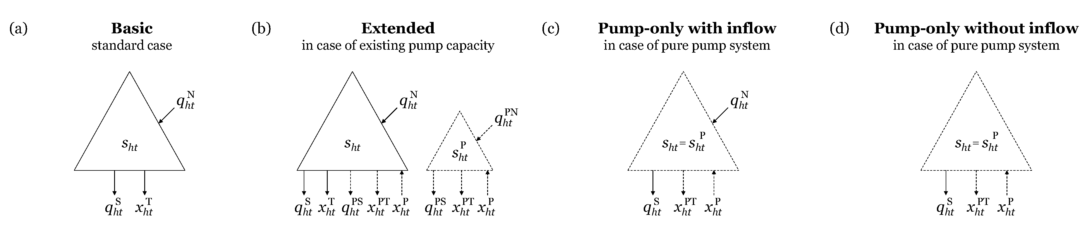
Before going into the formulations of the equivalent hydro system model, it is convenient to review the proposed model types that can become necessary to feature various configurations of detailed hydro systems. As shown in Figure 5, four different types of the equivalent hydro system model can be distinguished from each other.

The basic model type (a) represents a hydro system with one or more reservoirs which are only connected by conventional hydro turbines and spillage flows. Hence, aside from storing or spilling the natural energy inflow, it is only able to generate electricity (i.e., a conventional hydro storage or run-of-the-river system).

By including pumping capability, the extended model type (b) allows the equivalent model to also consume and store electricity. To not overestimate the flexibility of pumped-hydro storage, a second synthetic reservoir (dashed) is introduced to additionally limit the pump and pumped hydro turbine utilisation. Note that the conventional hydro turbine capacity (T) is distinguished from the pumped hydro turbine capacity (PT).

The pump-only model type is a special case since it is only applicable if the detailed hydro reservoir system does not feature any conventional hydro turbine capacity, or storage, for that matter. Thus, there is no need for an additional synthetic reservoir because the main reservoir already captures the full energy shifting potential. Depending on whether this model type possesses a natural inflow, two model types, either (c) or (d), have to be considered.

4.4. Equivalent Model Formulation

By using the conversion coefficients from Section 4.2, the amount of potential energy stored in the equivalent reservoir of hydro system h can be written as

$$s_{ht}=\sum _j^{J_h}{s}_{hjt}·{\pi }_{hj}^{\mathrm{T}}\forall h,t$$

(15)

where the equivalent reservoir level is subject to the lower and upper bounds:

$$s_h^{\min }\le s_{ht}\le s_h^{\max }\forall h,t$$

(16)

In the case of the extended equivalent hydro system model type, the storage capacity of the second synthetic hydro reservoir must only account for the detailed hydro reservoirs with pumping capacity connected to them. Hence, the subset of all pumped storage hydro reservoirs is defined as

$$J_h^{\mathrm{P}}=\left\{j\in J_h\mid I_{hj}^{\mathrm{DS}}\cap I_h^{\mathrm{P}}\ne ⌀\right\}\forall h$$

(17)

where $I_{hj}^{\mathrm{DS}}$ is the subset of all downstream (DS) hydro plants directly connected to hydro reservoir j, and $I_h^{\mathrm{P}}$ the subset of all hydro plants with pumping capacity of hydro system h, defined as

$$I_h^{\mathrm{P}}=\left\{i\in I_h\mid x_{hi}^{\mathrm{P},\max }>0\right\}\forall h$$

(18)

Moreover, the equivalent pumped storage level of a detailed hydro reservoir j is determined by the maximum conversion coefficient difference ${\pi }_{hj}^{\Delta }$ between its own average turbine conversion coefficient ${\pi }_{hj}^{\mathrm{T}}$ and the turbine conversion coefficients of its directly connected downstream reservoirs:

$$s_{ht}^{\mathrm{P}}=\sum _j^{J_h^{\mathrm{P}}}{s}_{hjt}·{\pi }_{hj}^{\Delta }\forall h,t$$

(19)

with

$${\pi }_{hj}^{\Delta }=\underset{{\widehat{j}}_{hik}}{max}\left({\pi }_{hj}^{\mathrm{T}}-{\pi }_{h{\widehat{j}}_{hik}}^{\mathrm{T}}·{\kappa }_{h{\widehat{j}}_{hik}}\right)i\in I_{hj}^{\mathrm{DS}},k\in K_{hij}$$

(20)

where ${\widehat{j}}_{hik}$ and ${\kappa }_{h{\widehat{j}}_{hik}}$ are in line with Equation (11), and the upper and lower storage level bounds correspond to Equation (16):

$$s_h^{\mathrm{P},\min }\le s_{ht}^{\mathrm{P}}\le s_h^{\mathrm{P},\max }\forall h,t$$

(21)

The natural inflow of potential energy to the equivalent reservoir of hydro system h is

$$q_{ht}^{\mathrm{N}}=\sum _j^{J_h}\left(q_{hjt}^{\mathrm{N}}·{\pi }_{hj}^{\mathrm{T}}-\sum _{\widehat{j}}^{J_{hj}^{\mathrm{DS}}}{q}_{hj\widehat{j}t}^{\mathrm{S}*}·\left({\pi }_{hj}^{\mathrm{T}}-{\pi }_{h\widehat{j}}^{\mathrm{T}}·{\kappa }_{h\widehat{j}}\right)\right)\forall h,t$$

(22)

where $q_{hj\widehat{j}t}^{\mathrm{S}*}$ is the unavoidable spillage resulting from the maximisation in Equation (14) and yielding a loss of potential energy between the spilling reservoir j and the spillage target reservoir $\widehat{j}$. Accordingly, the equivalent inflow to the pumped storage reservoir of the extended model type can be formulated as

$$q_{ht}^{\mathrm{PN}}=\sum _j^{J_h^{\mathrm{P}}}\left(q_{hjt}^{\mathrm{N}}·{\pi }_{hj}^{\Delta }-\sum _{\widehat{j}}^{J_{hj}^{\mathrm{DS}}}{q}_{hj\widehat{j}t}^{\mathrm{S}*}·\left({\pi }_{hj}^{\mathrm{T}}-{\pi }_{h\widehat{j}}^{\mathrm{T}}·{\kappa }_{h\widehat{j}}\right)\right)\forall h,t$$

(23)

which only accounts for the pumped storage reservoirs ($J_h^{\mathrm{P}}$), and credits their inflow by ${\pi }_{hj}^{\Delta }$ from Equation (20).

As with the detailed model, the spillage cannot be negative, which is ensured by the following constraints

$$0\le q_{ht}^{\mathrm{S}}0\le q_{ht}^{\mathrm{PS}}\forall h,t$$

(24)

where the main difference is that only one equivalent spillage variable $q_{ht}^{\mathrm{S}}$ is necessary for the whole hydro system. The additional pumped hydro spillage variable $q_{ht}^{\mathrm{PS}}$ is only required for the extended model type.

Note that $s_{ht}$, $s_{ht}^{\mathrm{P}}$, $q_{ht}^{\mathrm{N}}$, $q_{ht}^{\mathrm{PN}}$, $q_{ht}^{\mathrm{S}}$ and $q_{ht}^{\mathrm{PS}}$ are no longer measured in the amount of water (${\mathrm{hm}}^3$) but the amount of potential energy (MWh).

Since the hydraulic interconnection information within the hydro systems becomes obsolete in the explicit equivalent hydro system model formulation, only the energy in- and output variables need to be considered:

$$x_{ht}^{\mathrm{T}}=\sum _i^{I_h\backslash I_h^{\mathrm{PT}}}{x}_{hi}^{\mathrm{T}},x_{ht}^{\mathrm{T},\min }\le x_{ht}^{\mathrm{T}}\le x_{ht}^{\mathrm{T},\max }\forall h,t$$

(25)

$$x_{ht}^{\mathrm{PT}}=\sum _i^{I_h^{\mathrm{PT}}}{x}_{hi}^{\mathrm{T}},x_{ht}^{\mathrm{PT},\min }\le x_{ht}^{\mathrm{PT}}\le x_{ht}^{\mathrm{PT},\max }\forall h,t$$

(26)

$$x_{ht}^{\mathrm{P}}=\sum _i^{I_h^{\mathrm{P}}}{x}_{hi}^{\mathrm{P}},x_{ht}^{\mathrm{P},\min }\le x_{ht}^{\mathrm{P}}\le x_{ht}^{\mathrm{P},\max }\forall h,t$$

(27)

Here, the subset of all hydro plants with pumped hydro turbine capacity is

$$I_h^{\mathrm{PT}}=\left\{i\in I_{hj}^{\mathrm{DS}}\mid j\in J_h^{\mathrm{P}}\right\}\forall h$$

(28)

and is therefore not limited to the set defined by Equation (18), and rather includes all hydro plants directly connected downstream to all pumped storage reservoirs of a hydro system h, implying that their conventional turbine capacity can be used in a pump-turbine cycle.

In accordance with Equation (1), the active equivalent reservoir level becomes

$$s_{h{t}^{\prime }}=s_{ht}+q_{ht}^{\mathrm{N}}-x_{ht}^{\mathrm{T}}-x_{ht}^{\mathrm{PT}}+x_{ht}^{\mathrm{P}}·{\eta }_h^{\mathrm{P}}-q_{ht}^{\mathrm{S}}-q_{ht}^{\mathrm{PS}}\forall h,t$$

(29)

Similarly, the active storage level of the synthetic reservoir is denoted by

$$s_{h{t}^{\prime }}^{\mathrm{P}}=s_{ht}^{\mathrm{P}}+q_{ht}^{\mathrm{PN}}-x_{ht}^{\mathrm{PT}}+x_{ht}^{\mathrm{P}}·{\eta }_h^{\mathrm{P}}-q_{ht}^{\mathrm{PS}}\forall h,t$$

(30)

which is only relevant for the extended model type.

In both equivalent reservoir balance equations, the equivalent pump conversion coefficient is denoted as

$${\eta }_h^{\mathrm{P}}=\frac{1}{{\sum }_i^{I_h^{\mathrm{P}}}{x}_{hi}^{\mathrm{P},\max }}\sum _j^{J_h^{\mathrm{P}}}\sum _i^{I_h^{\mathrm{P}}\cap I_{hj}^{\mathrm{DS}}}\sum _k^{K_{hij}^{\mathrm{US}}}\frac{x_{hi}^{\mathrm{P},\max }}{\left|K_{hi}\right|}·\frac{{\pi }_{hj}^{\Delta }}{{\pi }_{hik}^{\mathrm{P}}}\forall h$$

(31)

where $K_{hij}^{\mathrm{US}}$ is the set of all downstream paths of pumped hydro plant i with an upstream connection to pumped hydro reservoir j, which is not to be confused with $K_{hi}$ denoting the set of all parallel paths of pumped hydro plant i, see Equation (10). The inner two sums essentially determine an equivalent pump conversion coefficient for each pumped storage reservoir $j\in J_h^{\mathrm{P}}$, proportional to the installed downstream pump capacity, and not disregarding potential parallel paths. The outer sum adds up the weighted equivalent pump conversion coefficients of every pumped storage reservoir which is then divided by the equivalent maximum pump capacity, presented in Equation (27).

In contrast to Equation (6), the equivalent pump conversion coefficient ${\eta }_h^{\mathrm{P}}$ describes the losses incurred during the entire pump and turbine operation cycle. Because the upper bound of $s_{ht}^{\mathrm{P}}$ is evaluated by the average turbine conversion coefficient in Equation (19), the combination of the equivalent pumped storage capacity and the equivalent pump conversion coefficient do not overestimate the overall pump cycle potential.

5. Clustered Equivalent Hydro System Model

Depending on the application, the equivalent hydro system model can already provide a sufficient reduction of complexity and computational burden. For instance, this is the case if the geographical scope only requires a small number of detailed, but highly complex hydro systems. However, since many applications, such as analysing the European power system, require the representation of a multitude of hydropower systems (see Figure 1), further aggregation can be necessary.

To that end, the core idea of the clustered equivalent hydro system model is to harness the fact that the instances of the uniforming model formulations in Section 4 can exhibit very similar characteristics. By clustering and merging these equivalent hydro units according to their coherent features, a further aggregation can be achieved.

Note that the model formulation of Section 4.4 remains the same, only the number of equivalent model instances is reduced.

5.1. Clustering Criteria

To identify the similarities among the equivalent hydro units, a set of four clustering criteria is used.

The first criterion is the inflow pattern of all relevant equivalent hydro units, i.e., the equivalent natural inflow profiles $q_{ht}^{\mathrm{N}}$. Their similarity is taken into account by explicitly including the normalised temporal sequences in the input data of the clustering process. By employing corresponding weights, the overall impact of the inflow pattern criterion is limited to an even contribution among the other active clustering criteria.

Determining the hydro reservoir’s ability to store natural inflow, the degree of regulation criterion is defined as

$${\alpha }_h=\frac{s_h^{\max }}{{\sum }_t^T{q}_{ht}^{\mathrm{N}}}\forall h$$

(32)

Determining the overall active storage capacity of an equivalent hydro system, the storage turbine ratio criterion is defined as

$${\beta }_h^{\mathrm{T}}=\frac{s_h^{\max }}{x_h^{\mathrm{T},\max }}\forall h$$

(33)

Determining the active storage capacity available for pumping of an equivalent hydro system, the storage pump ratio criterion is defined as

$${\beta }_h^{\mathrm{P}}=\frac{s_h^{\mathrm{P},\max }}{x_h^{\mathrm{P},\max }}\forall h$$

(34)

According to

Table 1. Model types and active criteria when clustering equivalent hydro models (active criteria indicated by •).

Model Type	Inflow Pattern	${\mathit{\alpha }}_{\mathit{h}}$	${\mathit{\beta }}_{\mathit{h}}^{\mathbf{T}}$	${\mathit{\beta }}_{\mathit{h}}^{\mathbf{P}}$
Basic	•	•	•	-
Extended	•	•	•	•
Pump-only with inflow	•	•	•	•
Pump-only without inflow	-	-	•	•

, the criteria being active in the clustering process differ depending on the model type.

The clustering process is carried out for each equivalent model type in each considered market area in Europe. Depending on a market area’s structure of hydro systems, the clustering step can yield a varying degree of aggregation benefits. For instance, a market area with numerous hydro systems, each consisting only of a few hydro reservoirs and plants, will result in the same number of equivalent hydro systems, still leaving some aggregation opportunity for the clustering process. Conversely, a market area with only a few hydro systems, each composed of multiple hydro reservoirs and plants, experiences the main aggregation benefits while building the equivalent hydro system model and does not present much additional potential for aggregation (see the number of detailed hydro reservoirs and plants compared to the number of equivalent and clustered equivalent hydro systems in

Table 2. Hydropower characteristics for all three model variants based on the collected bottom-up data for all considered market areas across Europe.

Market Area	Total Capacity in GW			Total Storage Capacity in TWh		Number of
	Turbine (T)	Pumped Hydro	Pump	Equivalent	Equivalent	Detailed	Detailed	Equivalent	Clustered eq.
		Turbine (PT)	(P)	Storage${}^{+}$	Pumped Storage${}^{+}$	Hydro Plants	Hydro Reservoirs	Hydro Systems	Hydro Systems
AUT	8.32	5.54	4.49	(3.21)	(1.02)	176	236	61	14
BEL	0.11	1.30	1.20	(0.02)	(0.01)	13	24	11	3
CHE	12.30	6.50	5.51	(10.12)	(2.10)	153	207	68	16
CZE	1.09	1.15	1.13	(0.34)	(0.03)	23	38	15	6
DEU	4.67	10.12	8.88	(0.48)	(0.11)	150	185	40	9
ESP	11.44	10.81	9.19	(17.58)	(3.60)	405	458	94	18
FIN	3.23	-	-	(5.22)	-	113	133	27	7
FRA	18.11	6.08	4.82	(8.53)	(0.74)	296	358	56	14
GBR	1.34	4.14	3.90	(1.41)	(0.08)	64	88	22	12
HUN	0.07	-	-	(<0.01)	-	4	8	4	2
IRL	0.24	0.72	0.72	(0.09)	(<0.01)	14	24	10	6
ITA	15.87	6.84	6.87	(11.63)	(0.32)	484	608	137	15
LUX	0.05	-	-	(<0.01)	(<0.01) *	5	6	3	2
NLD	0.05	-	-	(<0.01)	-	5	10	5	2
NOR	30.51	1.37	1.04	(82.41)	(2.36)	382	500	120	20
POL	0.55	1.76	1.65	(0.12)	(0.05)	18	32	14	9
PRT	5.19	4.22	3.28	(4.66)	(0.92)	65	70	13	8
SVK	1.85	1.62	1.62	(0.63)	(0.06)	34	42	9	5
SVN	1.57	0.58	0.62	(0.02)	(<0.01)	35	37	4	2
SWE	16.34	-	-	(32.16)	-	221	243	21	7
ALL	132.90	62.74	54.89	(178.64)	(11.42)	2660	3307	734	177

${}^{+}$ Total storage and pump storage capacity figures can merely be used as an indication since structural and inflow information is vital to the allocation of storage capacity among the hydro systems in one market area. * The pump storage reservoir capacity is geographically located in market area LUX, but the total pump turbine and pump capacities participate in market area DEU.

).

It has to be mentioned that hydro systems with a total turbine capacity below a minimum threshold of either 0.2% of the market area’s total installed capacity (relative threshold) or 10 MW (absolute threshold) are left out of the clustering process to avoid distortions. After the clustering procedure, those small hydro systems are allocated to the centroid closest to them.

5.2. Clustering Algorithm

Finding appropriate clusters in data sets is a standard problem which has been approached by a variety of methods. Here, the common k-means clustering technique using the squared Euclidean distance is employed. It is an iterative data-partitioning algorithm [41] (or Lloyd’s algorithm [42]) assigning n observations to exactly one of k clusters defined by centroids. Through this process, subsets of the full data set are created and the centroid of each subset corresponds to the mean of all measurements belonging to it.

As the number of clusters needs to be chosen beforehand, the clustering algorithm is run for multiple numbers, after which a knee-point detection is used. Finding good local minimums is ensured by repeating the clustering several times (100 replicates). Moreover, it is important to standardise the values of the criteria to a specific range in the preprocessing stage of the clustering procedure. In this context, the z-score standardisation method is used.

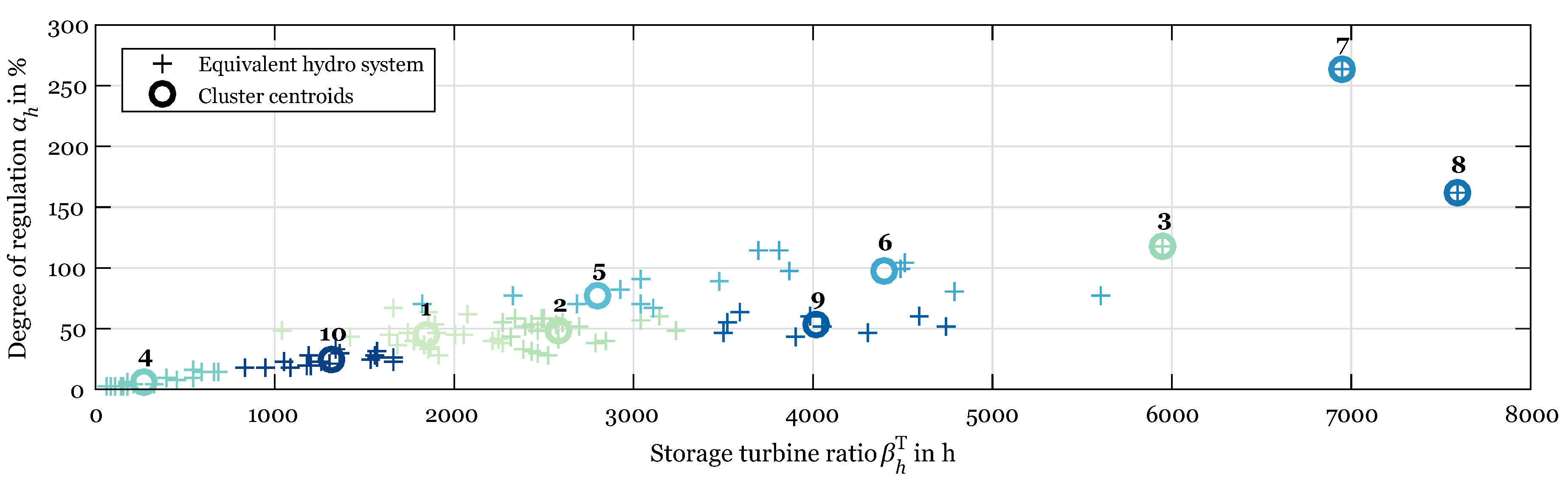
To give an illustration, Figure 6 depicts the clustering results for the basic model type, i.e., run-of-the-river and conventional storage hydro systems with natural inflow, in Norway (climate reference year 2011).

Note that, for the sake of clarity, the inflow pattern criterion is not shown in this diagram, but it is used during the clustering procedure. Inspecting the equivalent hydro systems of clusters, e.g., 1, 5, and 10, clearly reveals that the inflow pattern has an impact on the grouping results of the clustering procedure. As becomes obvious, the clustering process determined ten clustered equivalent hydro units.

5.3. Merging Clustered Units

It is important to stress that the cluster centroids (circles) in Figure 6 are only to be interpreted as an indication as to which equivalent hydro units are grouped together.

Setting up the clustered equivalent hydro system units is fairly straight-forward because almost all equivalent hydro model parameters belonging to an identified cluster are simply summed up. This means that the equivalent storage, pumped storage level, natural inflow profiles, as well as turbine, pumped hydro turbine, pump capacities are each summarised to their clustered equivalent values.

For each clustered equivalent unit, however, the pump conversion coefficient ${\eta }_h^{\mathrm{P}}$ is calculated as a mean, weighted by the installed equivalent pump capacity. What is more, the market area participation coefficients of each clustered equivalent hydro unit is updated to meet the turbine, pumped hydro turbine, and pump capacity allocation of the equivalent hydro units it aggregates.

6. Case Study

The following case study analysis presents a comparison of both the equivalent and clustered equivalent hydro system model with the detailed reference hydro system model. With that in mind, a power market simulation for the European energy market is carried out to identify the differences induced by using different levels of hydropower aggregation. Its objective is to minimise the operational costs of the power system including the interactions with the heat and transport sectors.

6.1. Scenario Description

The analysis is based on a decarbonised energy scenario for Europe with significant coupling of power, heat, industry, and transport sectors. This cost-optimised target scenario for 2050 is a result of the SCOPE model which is continually being developed at Fraunhofer IWES. A detailed formulation of the model is given in [43], and [44] contains a detailed input data description. Minimising system operation and investment costs, while at the same time complying with a given carbon emission target covering all relevant sectors, this deterministic generation expansion planning model is formulated as a linear program (LP) for a full consecutive year (chronological 8760 h). All time series data depending on meteorological information, e.g., wind and solar production, thermal and cooling loads, etc., is based on COSMO-EU data [45].

By targeting a 95% reduction of carbon emissions in Europe by 2050 below 1990 levels (Kyoto Protocol accounting rules), the scenario primarily needs the remaining 5% for non-energy emissions. Regarding the transport sector, key assumptions are based on [46] by assuming a moderate increase in transport performance and an overall share of electric vehicles in the amount of 85% by 2050. As described in [44], the heating demands for both buildings and industry processes are subject to high efficiency levels.

Table A1. Installed generation and flexibility capacity of decarbonised long-term energy scenario for all considered market areas in Europe.

Market Area	Renewable Generation Capacity in GW			Thermal Generation Capacity in GW				Storage Capacity in GW
	Wind Onshore	Wind Offshore	Solar PV${}^{+}$	Natural Gas	Natural Gas	Natural Gas	Nuclear	Battery Storage	Power-to-Gas
				OCGT	CCGT	CHP-CCGT*	Steam Turbine
AUT	9.6	-	46.2	-	-	-	-	0.8	-
BEL	4.8	6.0	48.4	-	6.5	4.9	-	3.1	-
CHE	2.0	-	53.6	-	-	-	-	4.1	-
CZE	23.9	-	26.3	-	-	4.0	1.9	0.2	-
DEU	112.3	31.9	192.4	3.3	-	22.2	-	6.6	-
DNK	16.0	6.0	6.1	-	-	1.8	-	0.5	2.2
ESP	91.5	0.7	121.2	-	-	3.8	-	6.8	4.3
FIN	18.2	6.0	-	0.5	-	3.6	1.6	0.6	-
FRA	158.4	2.0	156.0	-	-	11.1	7.6	9.2	7.7
GBR	76.7	38.3	177.6	2.2	5.8	17.7	-	18.8	5.1
HUN	7.1	-	8.9	-	-	1.2	-	-	-
IRL	10.2	3.9	13.0	0.3	0.4	2.0	-	1.3	2.1
ITA	63.8	0.7	204.9	-	-	-	-	27.6	-
LUX	0.7	-	3.8	-	2.9	0.2	-	-	-
NLD	20.6	14.5	58.5	0.7	-	6.8	-	6.0	-
NOR	-	5.0	-	-	-	0.7	-	-	0.7
POL	73.5	2.3	114.2	4.1	5.5	11.7	-	11.8	6.2
PRT	16.3	-	38.1	-	-	0.7	-	3.2	1.2
SVK	9.9	-	17.5	-	-	1.2	1.3	-	-
SVN	1.9	-	9.6	-	0.1	0.6	-	-	-
SWE	20.9	4.0	-	-	-	1.5	-	-	-

${}^{+}$ Shown values represent aggregate generation capacity of rooftop and utility-scale PV. * Flexible co-generation units, i.e. backup boiler and backup electric heating unit, with heat extraction for district and industry heating demands.

provides more detailed characteristics of the resulting power generation mix in every considered market area, i.e., installed renewable, thermal, and storage capacity.

6.2. Power Market Simulation

The power market simulation is based on [47,48] and represents a standard unit dispatch problem (LP formulation) minimising system operation cost, i.e., fuel, emission, and load change cost. Im- and export between the market areas is ensured by 2030 net transfer capacities based on [49]. Moreover, the heat market aggregation method proposed in [50] is employed to have an efficient implementation of the power and heat sector interactions. To efficiently account for future ties between the power and transport sector, the vehicle fleet model and aggregation presented in [43] is used. Carbon emissions are priced at 100€/${\mathrm{tCO}}_2$.

For the purpose of this study, a power market simulation for each of the three hydro system model variants is conducted:

• Detailed (reference)
• Equivalent
• Clustered equivalent

The case study is implemented in MATLAB R2016a (MathWorks, Natick, MA, USA) and the resulting optimisation problem is solved by ILOG CPLEX V12.6.3(IBM, Armonk, NY, USA) on a High-Performance Computing Cluster (CPU: $32\times 2.3$ GHz, RAM: 252 GB).The detailed reference problem consists of about 70.6 million continuous variables and 27.2 million constraints.

6.3. Results

6.3.1. Energy Production and Consumption

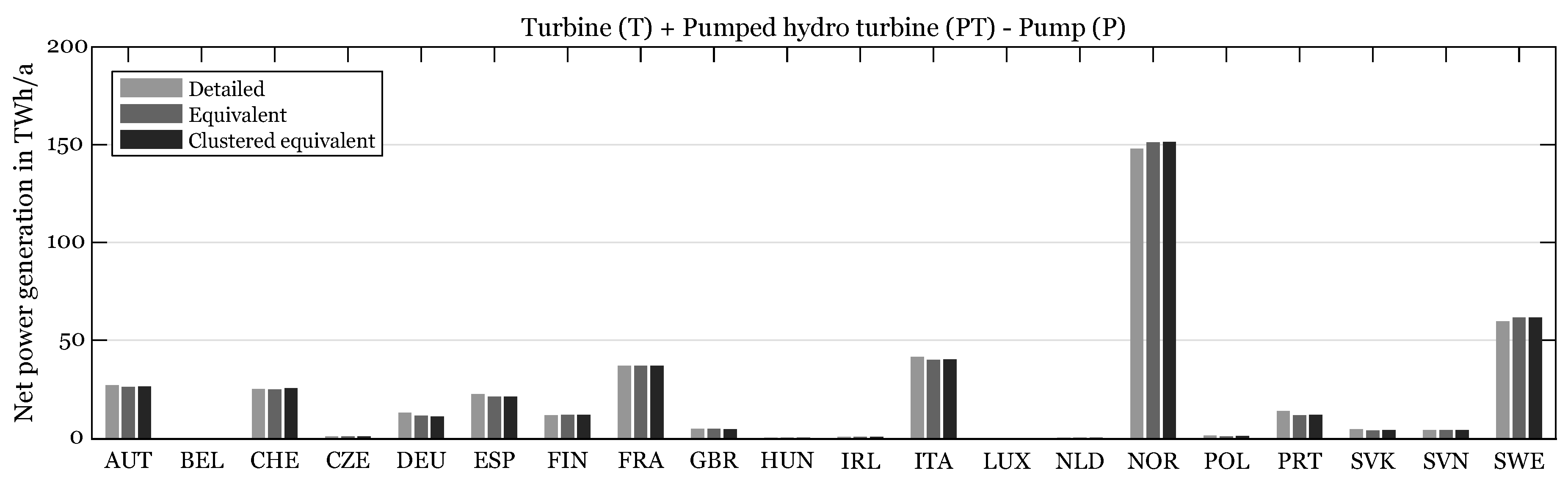
In Figure 7, the annual sum of net hydropower generation for all three model variants is given, i.e., turbine generation (T) plus pumped hydro turbine generation (PT) minus pump consumption (P).

Inspection of the resulting net generation figures reveals that, taken as a whole, there are only minor differences in net hydropower generation among the different levels of aggregation. Despite that, two aspects are noteworthy: first, NOR and SWE show slightly higher net generations while e.g., DEU, ESP, ITA and PRT exhibit small reductions in net generation for the more aggregated model variants; second, for AUT slight net generation reductions become visible, but only for the equivalent model variant. Moreover, BEL exhibits a negative net generation for all three model variants.

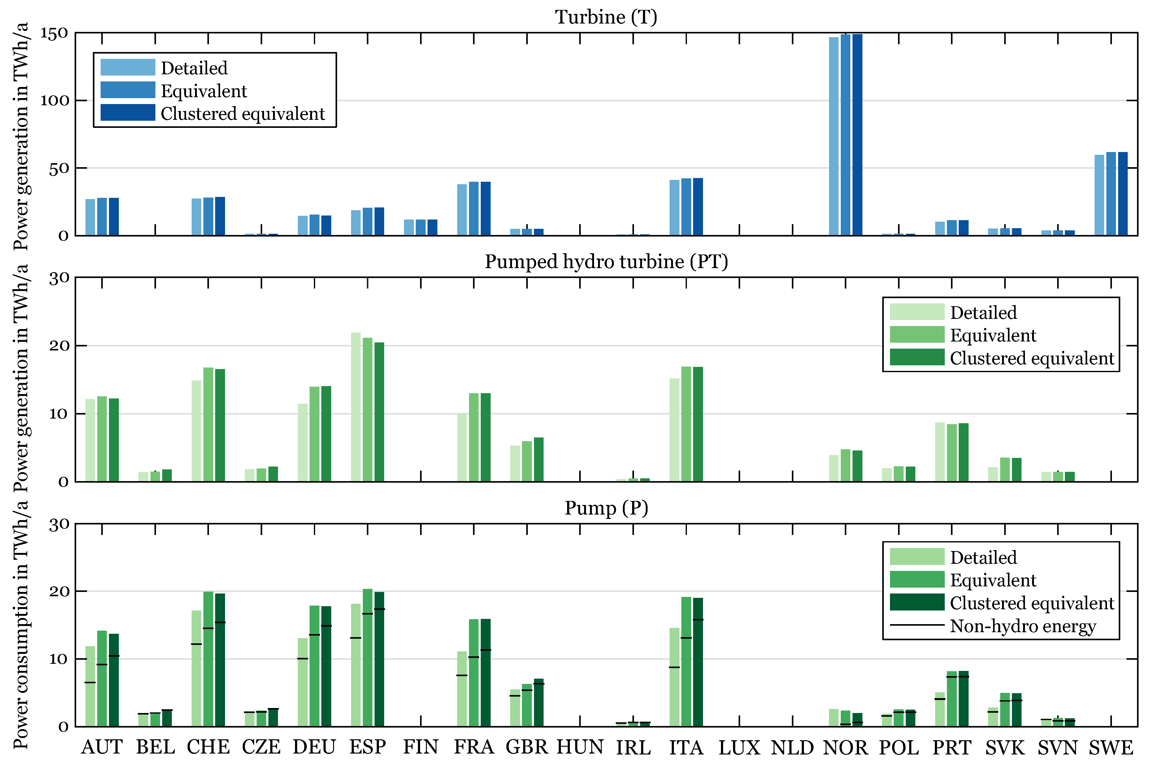
To better understand the above effects, a separate assessment of turbine generation, pumped hydro turbine generation, and pump consumption is given in Figure 8.

As can be seen from the comparison of annual turbine (T) generation, both the equivalent and clustered equivalent model variants exhibit marginally higher levels of production for almost all market areas, particularly those with significant conventional hydropower generation capacity.

The pumped hydro turbine (PT) generation tends to be higher for the aggregated model variants, although no clear pattern can be observed. More specifically, in many market areas, the pumped hydro turbine generation of the equivalent model is even higher than that of the clustered equivalent model variant. In the market area ESP, elevated pumped hydro turbine generation levels of the detailed model variant become evident.

Regarding the pattern of pump consumption (P), the annual energy demand of pumps generally shows higher values for the aggregated model variants and reflects the above observation of increased PT generation. Furthermore, the indicated share of non-hydro energy (black bars) reveals whether the energy output of hydro generation (T and PT), or non-hydro sources such as other renewable or conventional generation, are consumed during the pump cycles. As can be seen, the share of pumped non-hydro energy (below the bar) increases with the level of model aggregation. That said, the share of pumped energy from hydro generation (above the bar) does not exhibit a clear tendency. In some market areas, it is smallest for the clustered equivalent model variant, e.g., AUT, ESP, GBR, ITA, and NOR, while it is almost constant (POL) or increasing in others, such as FRA, SVK, and SVN.

6.3.2. Scheduling Decisions

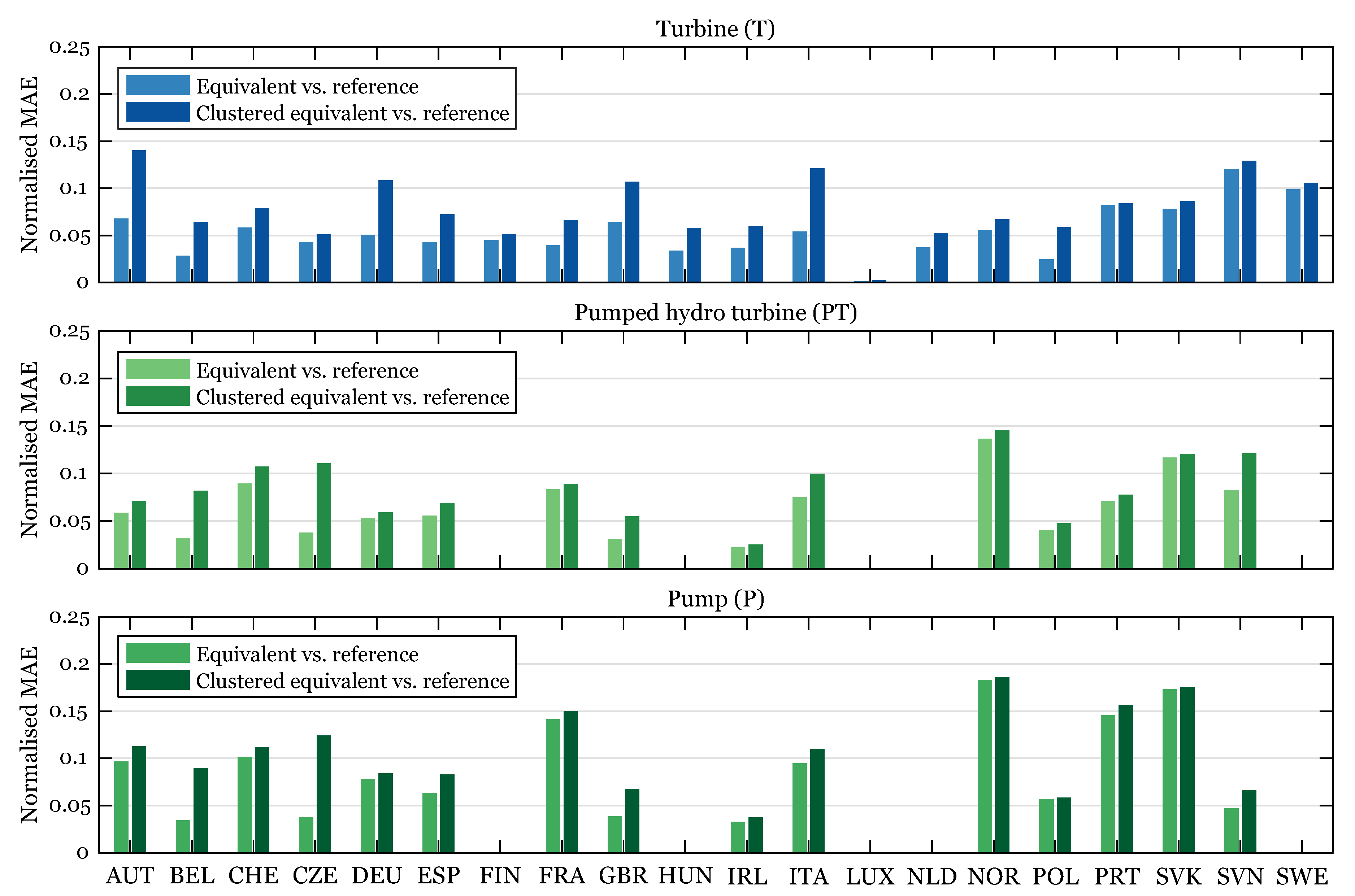
The resulting deviations in dispatching decisions from using the different model variants are illustrated with the Mean Absolute Error (MAE) in Figure 9.

The MAEs of turbine, pumped hydro turbine, and pump schedules, each normalised by the corresponding maximum capacity, indicate deviations of about 5–10% for the most part. In some cases, the deviations exceed 15%, but generally stay below 20%.

According to expectations, the deviations for the clustered equivalent hydro system model are always higher than the deviations caused by the equivalent model variant. Most significantly, these deviation differences can be observed for the turbine generation (T) for the market areas AUT, DEU, GBR, and ITA.

Schedule deviations of pumped hydro turbine generation and pump consumption reveal some level of correlation, although the normalised MAE of the pump consumption schedules tends to be slightly bigger.

6.3.3. Solution Time and Objective Value

To provide results relevant to the pivotal task of finding adequate but computationally efficient hydropower representations, the observed solution times and objective values are given in

Table 3. Comparison of solution time and objective values.

Model Variant	Solution Time		Objective Value
	In h	% of Reference	In bn€	% of Reference
Detailed	42.9	100.0	23.1	100.0
Equivalent	4.7	10.9	21.7	94.2
Clustered equivalent	0.5	1.3	21.2	92.0

.

As intended, both aggregated model formulations yield considerable reductions in solution time. While a reduction to about 11% can be observed for the equivalent model variant, the optimisation problem with the clustered equivalent model solves almost eighty times faster than the detailed reference.

Regarding the objective value, deviations of about 6% and 8% in system operation cost occur for the equivalent and clustered equivalent model implementation, respectively.

7. Discussion

7.1. Limitations

There are a few simplifications and assumptions which need to be transparent when interpreting the results of this analysis.

Most notably, the detailed unit model presented in Section 3 already constitutes a simplified representation of the hydropower complex across Europe. Due to a lack of consistently available micro-level data, it had to be built on the basis of publicly accessible information. Also, it has to be stressed that the hydro reservoirs’ natural inflow profiles are based on the runoff parameter of the ERA-Interim model in combination with average historical or planned production data. This can only be seen as an approximation, but it offers a necessarily generic approach towards the even more problematic issue of inflow data availability.

Regarding the model, a deterministic linear model of a hydropower system is built, which neither accounts for head variations nor the travel of water. Given the high level focus on power markets, the aforementioned data availability, and the purpose of this comparison exercise, this modelling approach is deemed appropriate. Moreover, participation in balancing markets is not considered in this comparison, but it could be easily incorporated into the equivalent hydro system models.

Furthermore, geographical locations, other than the market area affiliation, are not considered in the clustering procedure. However, the clustering criteria could easily be extended to include this type of information.

A general simplification is to suppose that the natural inflows are known for the entire planning horizon. This commonly made assumption is very debatable [15] and has lead to specialised implementations involving stochastic optimisation. Though, the main purpose of the presented aggregation approach is to be used in planning and investment problems with a sufficient representation of operational flexibility, rather than in detailed generation planning problems for a single hydro valley. Coupled with the fact that the same assumption is often made for e.g., the electricity demand, as well as renewable generation in these kinds of models, the perfect foresight assumption is deemed appropriate here.

Altogether, it has to be kept in mind that the state aggregation method’s dominant difficulty is the loss of information that occurs during the aggregation process [8], which is an inevitable price to pay if the computational burden is to be reduced.

7.2. Aggregation Effects

Comparing the equivalent and clustered equivalent against the detailed hydro system model under the highly decarbonised energy scenario, it can be observed that the net power generation of hydro systems in Europe only slightly varies and therefore gives a reasonable accuracy. Minor positive deviations result from better utilisation of accumulated storage capacity and aggregated natural inflow. Negative deviations can be attributed to increased pumped hydro cycles for the aggregated model variants. These observations can be confirmed by the individual energy generation and consumption comparison in Section 6.3.1.

Because the pumped hydro turbine (PT) releases energy from both natural inflow and previously pumped water, interpreting its annual generation level is more intricate in comparison. This essentially means that the pumped hydro turbine generation balance is not entirely reflected by the pump consumption pattern, as is the case for e.g., AUT, PRT, and ESP.

An explanation for the elevated pump consumption (P) of the equivalent hydro system model variant is the hydro and non-hydro energy shares. In almost all market areas, the share of non-hydro energy used by pumping cycles goes up for both the equivalent and, even more so, the clustered equivalent hydro system model. The system uses the additional flexibility introduced by the aggregation measures to facilitate a better integration of non-hydro energy generation and consumption. At the same time, the share of hydro energy used while pumping remains relatively high for the equivalent model, but is particularly low for the clustered equivalent model variant. In other words, the increased level of aggregation leads to a situation in which heterogeneous hydro units within a market area see less and less need to balance each other, i.e., pump operation of one hydro unit while another is releasing energy, because this can be done within the clustered equivalent hydro units.

It has been shown by the obtained schedule deviations that the scheduling decisions mostly deviate below 10% of installed capacity, depending on the market area. For the more aggregated clustered equivalent hydro system model, the scheduling deviations are generally higher, and in some market areas the difference in deviations is particularly visible. Hence, the deviations suggest that in those market areas the clustered equivalent model variant tends to make more aggregation errors than in others.

The above findings also support the observed deviations in objective value, which can mainly be explained by reduced utilisation levels of thermal power plants. A further reason for the smaller objective value is the reduced fuel consumption of heat generation units, i.e., co-generation units and backup boilers, because it is substituted by electric backup heating options such as heat pumps and direct heating elements, see Table A1 and [50]. It has to be stated, however, that the seemingly large relative deviations correspond to relatively low absolute operational cost figures. Given the scenario’s high degree of decarbonisation, thermal power plants across Europe only generate about 168 TWh/a of electricity. In fact, this number is even lower for the equivalent and clustered equivalent model variants, 155 and 149 TWh/a, respectively.

Although spillage results are not explicitly shown here, it can be said that spillage reduces with an increasing degree of aggregation. Battery storage utilisation is only mildly affected by the hydro aggregation since all market areas with battery storage units experience small cycle reductions in the future energy scenario. Summarising, the aggregation leads to expected, but slight overestimations of hydropower flexibility.

7.3. Performance of Aggregation Approach

It becomes clear that the aggregation approaches’ performance, to a non-negligible degree, depends on the composition of the hydro complex in a market area. In other words, the mix and allocation of storage, turbine, and pump capacity, their interconnection within the hydro systems, as well as the nature of inflow profiles have a relevant impact on the aggregation approach.

All things considered, both aggregation approaches show a good performance in the future energy scenario setting with a significant level of decarbonisation. When factoring in the savings in computation time, the clustered equivalent hydro system model yields significant complexity reductions while maintaining a reasonable level of accuracy.

8. Conclusions

On the basis of a bottom-up hydropower data base of European hydropower systems, novel implementations of equivalent and clustered equivalent hydro system models are presented and compared against the reference detailed hydro system model. The analysis of aggregated modelling approaches for hydropower in Europe suggests that both aggregated model variants yield significant reductions in computation time while keeping an adequate level of accuracy. Once an aggregation becomes inevitable, it can be concluded that the clustered equivalent hydro system model is worth the additional loss in accuracy to benefit from the significant gain in solution time. The aggregation methods can easily be applied in different model types and may also be helpful in the stochastic case. Future work could focus on more individualised clustering approaches in the considered market areas.

References

- Chen, D.; Leon, A.S.; Gibson, N.L.; Hosseini, P. Dimension reduction of decision variables for multireservoir operation: A spectral optimization model. Water Resour. Res. 2016, 52, 36–51. [Google Scholar] [CrossRef]
- Nandalal, K.D.W.; Bogárdi, J.J. Dynamic Programming Based Operation of Reservoirs: Applicability and Limits; International Hydrology Series; Cambridge University Press: Cambridge, UK, 2013. [Google Scholar]
- Rogers, D.F.; Plante, R.D.; Wong, R.T.; Evans, J.R. Aggregation and Disaggregation Techniques and Methodology in Optimization. Oper. Res. 1991, 39, 553–582. [Google Scholar] [CrossRef]
- Korpås, M.; Warland, L.; Tande, J.O.G.; Uhlen, K.; Purchala, K.; Wagemans, S. Further Developing Europe’s Power Market for Large Scale Integration of Wind Power: D3.2 Grid Modelling and Power System Data; Technical Report; TradeWind: Oslo, Norway, 2007. [Google Scholar]
- Christensen, G.S.; Soliman, S.A. Optimal Long-Term Operation of Electric Power Systems; Mathematical Concepts and Methods in Science and Engineering; Springer: Boston, MA, USA, 1988; Volume 38. [Google Scholar]
- Fosso, O.B.; Gjelsvik, A.; Haugstad, A.; Mo, B.; Wangensteen, I. Generation scheduling in a deregulated system. The Norwegian case. IEEE Trans. Power Syst. 1999, 14, 75–81. [Google Scholar] [CrossRef]
- Wolfgang, O.; Haugstad, A.; Mo, B.; Gjelsvik, A.; Wangensteen, I.; Doorman, G. Hydro reservoir handling in Norway before and after deregulation. Energy 2009, 34, 1642–1651. [Google Scholar] [CrossRef]
- Labadie, J.W. Optimal Operation of Multireservoir Systems: State-of-the-Art Review. J. Water Resour. Plan. Manag. 2004, 130, 93–111. [Google Scholar] [CrossRef]
- Brandão, J.L.B. Performance of the Equivalent Reservoir Modelling Technique for Multi-Reservoir Hydropower Systems. Water Resour. Manag. 2010, 24, 3101–3114. [Google Scholar] [CrossRef]
- Salas, J.D.; Hall, W.A.; Smith, R.A. Disaggregation and Aggregation of Water Systems. In Operation of Complex Water Systems; Guggino, E., Rossi, G., Hendricks, D., Eds.; Springer: Dordrecht, The Netherlands, 1983; pp. 35–60. [Google Scholar]
- Morlat, G. Sur La Consigne D’exploitation Optimum Des Réservoirs Saisonniers. La Houille Blanche 1951, 4, 497–510. [Google Scholar] [CrossRef]
- Arvanitidits, N.; Rosing, J. Composite Representation of a Multireservoir Hydroelectric Power System. IEEE Trans. Power Appar. Syst. 1970, PAS-89, 319–326. [Google Scholar] [CrossRef]
- Saad, M.; Turgeon, A.; Bigras, P.; Duquette, R. Learning disaggregation technique for the operation of long-term hydroelectric power systems. Water Resour. Res. 1994, 30, 3195–3202. [Google Scholar] [CrossRef]
- Hall, W.A. Optimal state dynamic programming for multireservoir hydroelectric systems; Class Notes; Colorado State University: Fort Collins, CO, USA, 1971. [Google Scholar]
- Turgeon, A. Optimal operation of multireservoir power systems with stochastic inflows. Water Resour. Res. 1980, 16, 275–283. [Google Scholar] [CrossRef]
- Valdés, J.B.; Filippo, J.D.; Strzepek, K.M.; Restrepo, P.J. Aggregation-disaggregation approach to multireservoir operation. J. Water Resour. Plan. Manag. 1992, 118, 423–444. [Google Scholar] [CrossRef]
- Kularathna, M.D.U.P. Application of Dynamic Programming for the Analysis of Complex Water Resources Systems: A Case Study on the Mahaweli River Basin Development in Sri Lanka. Ph.D. Thesis, Landbouwuniversiteit Wageningen, Wageningen, The Netherlands, 1992. [Google Scholar]
- Turgeon, A.; Charbonneau, R. An aggregation-disaggregation approach to long-term reservoir management. Water Resour. Res. 1998, 34, 3585–3594. [Google Scholar] [CrossRef]
- Söder, L. Two-station equivalent of hydro power systems. In Proceedings of the 15th Power Systems Computation Conference (PSCC), Liege, Belgium, 22–26 August 2005; pp. 1–7. [Google Scholar]
- Maceira, M.E.P.; Duarte, V.S.; Penna, D.D.J.; Tcheou, M.P. An approach to consider hydraulic coupled systems in the construction of equivalent reservoir model in hydrothermal operation planning. In Proceedings of the 17th Power Systems Computation Conference (PSCC), Stockholm, Sweden, 22–26 August 2011. [Google Scholar]
- Dereu, G.; Grellier, V. Latest Improvements of EDF Mid-Term Power Generation Management. In Handbook of Power Systems I; Rebennack, S., Pardalos, P.M., Pereira, M.V.F., Iliadis, N.A., Eds.; Springer: Berlin/Heidelberg, Germany, 2010; pp. 77–94. [Google Scholar]
- Bellman, R. E. Dynamic Programming; Princeton University Press: Princeton, NJ, USA, 1957. [Google Scholar]
- Pereira, M.V.F.; Pinto, L.M.V.G. Multi-stage stochastic optimization applied to energy planning. Math. Program. 1991, 52, 359–375. [Google Scholar]
- Gjerden, K.S.; Helseth, A.; Mo, B.; Warland, G. Hydrothermal scheduling in Norway using stochastic dual dynamic programming; a large-scale case study. In Proceedings of the 2015 IEEE Eindhoven PowerTech, Eindhoven, The Netherlands, 29 June–2 July 2015; pp. 1–6. [Google Scholar]
- Hecker, C.; Zauner, E.; Pellinger, C.; Carr, L.; Hötzl, S. Modellierung der flexiblen Energiebereitstellung von Wasserkraftwerken in Europa. In Proceedings of the 9th Internationale Energiewirtschaftstagung (IEWT), Vienna, Austria, 11–13 February 2015. [Google Scholar]
- Hirth, L. The benefits of flexibility: The value of wind energy with hydropower. Appl. Energy 2016, 181, 210–223. [Google Scholar] [CrossRef]
- Korpås, M.; Trötscher, T.; Völler, S.; Tande, J.O. Balancing of Wind Power Variations Using Norwegian Hydro Power. Wind Eng. 2013, 37, 79–95. [Google Scholar] [CrossRef]
- Rede Eléctrica Nacional. Hidroelectricidade em Portugal: Memória e desafio; Rede Eléctrica Nacional: Lisbon, Portugal, 2002. [Google Scholar]
- SSE. Booklet Power from the Glens; SSE: Perth, UK, 2012. [Google Scholar]
- Confederación Hidrográfica del Júcar. Parte Estado Embalses; Confederación Hidrográfica del Júcar: Valencia, Spain, 2017. [Google Scholar]
- Terna Group. Spreadsheet; Terna Group: Roma, Italy, 2011. [Google Scholar]
- Energiavirasto. Power Plant Register; Energiavirasto: Helsinki, Finland, 2017. [Google Scholar]
- Norges Vassdrags- og Energidirektorat. NVE Atlas; Norges Vassdrags- og Energidirektorat: Oslo, Norway, 2015. [Google Scholar]
- Bundesamt für Landestopografie Swisstopo. Swiss Geoportal; Bundesamt für Landestopografie Swisstopo: Bern, Switzerland, 2017. [Google Scholar]
- EDF. Carte de nos Implantations Industrielles en France; EDF: Paris, France, 2017. [Google Scholar]
- Electrabel GDF Suez. La Centrale D’accumulation Par Pompage de Coo—Trois-Ponts: Et Les Centrales Hydroélectriques du Sud-Est de la Belgique; Electrabel GDF Suez: Brussels, Belgium, 2012. [Google Scholar]
- First Hydro. First Hydro Power Stations; First Hydro: Caernarfon, UK, 2017. [Google Scholar]
- European Centre for Medium-Range Weather Forecasts (ECMWF). ERA Interim, Daily; European Centre for Medium-Range Weather Forecasts (ECMWF): Reading, UK, 2015. [Google Scholar]
- Dee, D.P.; Uppala, S.M.; Simmons, A.J.; Berrisford, P.; Poli, P.; Kobayashi, S.; Andrae, U.; Balmaseda, M.A.; Balsamo, G.; Bauer, P.; et al. The ERA-Interim reanalysis: Configuration and performance of the data assimilation system. Q. J. R. Meteorol. Soc. 2011, 137, 553–597. [Google Scholar] [CrossRef]
- Wangensteen, I. Power System Economics: The Nordic Electricity Market; Tapir Academic Press: Trondheim, Norway, 2007. [Google Scholar]
- MacQueen, J.B. Some methods for classification and analysis of multivariate observations. In Fifth Berkeley Symposium on Mathematical Statistics and Probability; Le Cam, L.M., Neyman, J., Eds.; University of California Press: Berkeley, CA, USA, 1967; Volume 1, pp. 281–297. [Google Scholar]
- Lloyd, S. Least squares quantization in PCM. IEEE Trans. Inf. Theory 1982, 28, 129–137. [Google Scholar] [CrossRef]
- Trost, T. Erneuerbare Mobilität im motorisierten Individualverkehr: Modellgestützte Szenarioanalyse der Marktdiffusion alternativer Fahrzeugantriebe und deren Auswirkungen auf das Energieversorgungssystem. Ph.D. Thesis, Universität Leipzig, Stuttgart, Germany, 2017. [Google Scholar]
- Gerhardt, N.; Böttger, D.; Trost, T.; Scholz, A.; Pape, C.; Gerlach, A.K.; Härtel, P.; Ganal, I. Analyse Eines Europäischen-95%-Klimazielszenarios über Mehrere Wetterjahre: Teilbericht; Technical Report; Fraunhofer IWES: Kassel, Germany, 2017. [Google Scholar]
- Deutscher Wetterdienst. Numerische Vorhersagemodelle: Regionalmodell COSMO-EU; Deutscher Wetterdienst: Offenbach, Germany, 2016. [Google Scholar]
- Capros, P.; de Vita, A.; Tasios, N.; Siskos, P.; Kannavou, M.; Petropoulos, A.; Evangelopoulou, S.; Zampara, M.; Papadopoulos, D.; Nakos, C. EU Reference Scenario 2016: Energy, Transport and GHG Emissions: Trends to 2050; Technical Report; European Commission: Brussels, Belgium, 2016. [Google Scholar]
- Von Oehsen, A. Entwicklung und Anwendung Einer Kraftwerks- und Speicherinsatzoptimierung für Die Untersuchung von Energieversorgungsszenarien mit Hohem Anteil Erneuerbarer Energien in Deutschland. Ph.D. Thesis, Universität Kassel, Kassel, Germany, 2012. [Google Scholar]
- Jentsch, M. Potenziale von Power-to-Gas Energiespeichern: Modellbasierte Analyse des Markt- und Netzseitigen Einsatzes im Zukünftigen Stromversorgungssystem. Ph.D. Thesis, Universität Kassel, Kassel, Germany, 2015. [Google Scholar]
- Anderski, T.; Surmann, Y.; Stemmer, S.; Grisey, N.; Momot, E.; Leger, A.C.; Betraoui, B.; van Roy, P. European Cluster Model of the Pan-European Transmission Grid: E-HIGHWAY 2050: Modular Development Plan of the Pan-European Transmission System 2050; Technical Report; e-Highway2050: Puteaux, France, 2014. [Google Scholar]
- Härtel, P.; Sandau, F. Aggregated modelling approach of power and heat sector coupling technologies in power system models. In Proceedings of the 14th International Conference on the European Energy Market (EEM), Dresden, Germany, 6–9 June 2017; pp. 1–6. [Google Scholar]
Figure 1.
Map of detailed hydro plants (2660 in total) and hydro reservoirs (3307 in total) across the covered market areas in Europe.
Figure 2.
Classification of multistage reservoir systems into serial, branched, parallel, and parallel-branched hydro systems.
Figure 3.
Simulated hourly natural inflow profiles of two exemplary hydro reservoirs in Spain and Norway for the meteorological years 2000–2013 (February break indicates missing day of data for non-leap years).
Figure 4.
(a) Schematic illustration of parallel up- and downstream hydro plant connections; and (b) overview of the detailed hydro reservoir model.
Figure 5.
Four equivalent hydro system model types.
Figure 6.
Clustering results for the basic clustering category in market area NOR.
Figure 7.
Annual sum of net hydropower generation of detailed, equivalent, and clustered equivalent hydro system models in all considered market areas.
Figure 8.
Annual sum of energy generation and consumption of detailed, equivalent, and clustered equivalent hydro system models in all considered market areas (black bars display share of non-hydro energy consumption of pumps).
Figure 9.
Normalised mean absolute error (MAE) of turbine, pumped hydro turbine, and pump schedules for equivalent and clustered equivalent vs. detailed reference model variant in all considered market areas.