Battery Energy Management in a Microgrid Using Batch Reinforcement Learning †


1
ESAT/Electa, KU Leuven, Kasteelpark Arenberg 10 bus 2445, BE-3001 Leuven, Belgium
2
Energy Department, EnergyVille, Thor Park, Poort Genk 8130, 3600 Genk, Belgium
3
Energy Department, Vlaamse Instelling voor Technologisch Onderzoek (VITO), Boeretang 200, B-2400 Mol, Belgium
*
Author to whom correspondence should be addressed.
†
This paper is an extended version of our paper published in International workshop of Energy-Open 2017.
Energies 2017, 10(11), 1846; https://doi.org/10.3390/en10111846
Submission received: 15 October 2017
/
Revised: 5 November 2017
/
Accepted: 7 November 2017
/
Published: 12 November 2017
(This article belongs to the Special Issue Selected Papers from International Workshop of Energy-Open)
Abstract
:Motivated by recent developments in batch Reinforcement Learning (RL), this paper contributes to the application of batch RL in energy management in microgrids. We tackle the challenge of finding a closed-loop control policy to optimally schedule the operation of a storage device, in order to maximize self-consumption of local photovoltaic production in a microgrid. In this work, the fitted Q-iteration algorithm, a standard batch RL technique, is used by an RL agent to construct a control policy. The proposed method is data-driven and uses a state-action value function to find an optimal scheduling plan for a battery. The battery’s charge and discharge efficiencies, and the nonlinearity in the microgrid due to the inverter’s efficiency are taken into account. The proposed approach has been tested by simulation in a residential setting using data from Belgian residential consumers. The developed framework is benchmarked with a model-based technique, and the simulation results show a performance gap of 19%. The simulation results provide insight for developing optimal policies in more realistically-scaled and interconnected microgrids and for including uncertainties in generation and consumption for which white-box models become inaccurate and/or infeasible.
1. Introduction
The liberalization of the electricity market and environmental concerns have introduced new challenges in the design and operation of power grids [1]. As such, climate and energy packages adopted worldwide have resulted in clear objectives for the energy sector. For example, the European Union “climate and energy package” has set ambitious sustainability targets with the aim of halving greenhouse gas emissions to mitigate climate change by 2050 compared to 1990 [2], resulting in heavy investments in Renewable Energy Sources (RES) and power grid infrastructure. This has led to the smart grid paradigm, with technological advancement towards a green, intelligent and more efficient power grid. Microgrids can be a good base for the study and implementation of smart grid solutions [3,4,5]. Microgrids are electrical systems consisting of loads and distributed energy resources (like energy storage facilities and RES) that can operate in parallel with or disconnected from the main utility grid [6]. It is expected that the future power grid will be a combination of multiple microgrids collaborating with each other [7,8].
Over the years, the decreasing costs of Photovoltaic (PV) systems have led to the development of microgrids powered by PV systems [8]. However, one of the major challenges in operating microgrids powered by RES is to find energy management strategies, capable of handling uncertainties related to electricity production from RES and consumption. Recent technological innovations are producing batteries with improved storage capacities to bridge this gap [9]. The operation mode of energy storage devices has a major influence on the dynamics of microgrids. Thus, to ensure reliability and stability within the microgrid, there is a need to develop smart control strategies for energy storage devices in microgrids.
The traditional control paradigm is model-based, requiring an explicit model of the microgrid, a forecasting technique and an optimizer or a solver. Developing a model-based controller requires the selection and estimation of precise models and model parameters. In the microgrid setting, obtaining these models and parameters can be challenged by the heterogeneous and dynamic nature of electricity usage patterns and the intermittent nature of RES [10]. Thus, different electricity consumers might lead to completely different model parameters and perhaps different models. The implementation of model-based controllers on a large-scale requires the construction of appropriate models and corresponding model parameters and, as such, relies on expert knowledge. These factors mean that model-based solutions are not cost effective. Hence, model-based control approaches fail to provide effective solutions to achieve the desired control while minimizing implementation costs. One of the most successful and popular model-based control approaches is model predictive control [11]. Model predictive control was originally designed to solve open-loop deterministic optimal control problems in a receding horizon [12]. Despite the above-mentioned challenges, the works of Bifaretti et al. [13] and Prodan et al. [14] present a successful implementation of model predictive control to maximize self-consumption of locally-produced renewable energy in a microgrid. Another type of model-based control formulates the control problem as a Markov Decision Process (MDP) and solves the underlying optimization problem using dynamic programming techniques [15]. In the work of Costa et al. [16], a dynamic programming approach is used to solve a microgrid energy resource scheduling problem.
Unlike model-based control approaches, Reinforcement Learning (RL) techniques [17] are model-free and do not require system identification. Reinforcement learning techniques were designed to construct closed-loop policies for stochastic optimal control problems from a set of trajectories obtained from interactions with the real environment or from simulations. Hence, RL techniques are data-driven. With the development of smart grids, data on consumption patterns and electricity generation will be readily available making data-driven techniques relevant. This data availability together with the complex and stochastic nature of smart electricity grids makes data-driven methods more relevant to consider in smart grid control. Developing models for such large complex systems is difficult and costly, whereas the system model and dynamics could easily be learned from the readily available data. Ernst et al. [12] suggest that RL and model predictive control can complement each other to achieve robust and accurate optimal control. Q-learning, a temporal difference method and a popular on-line RL algorithm, has been applied in energy management in microgrids [3,18,19]. A bias-corrected Q-learning algorithm for efficient operation of energy storage devices during variations in electricity spot prices is proposed in the work of Lee et al. [20]. Kuznetsova et al. [18] proposed a framework for multi-criteria decision-making for energy storage management in a microgrid using Q-learning.
Despite being a popular RL method, Q-learning throws away the observations after every update, leading to inefficient data usage. This results in a slow convergence rate of the Q-learning algorithm to an optimal policy [21]; more observations are needed to construct a control policy. In batch RL techniques (off-line RL) [22,23], a controller estimates a control policy based on a batch of its past experiences. The ability of batch RL to reuse their past experiences makes them converge faster than online RL methods like Q-learning and SARSA. Batch RL has been used for demand response in [21,24,25,26]. Vandael et al. [27] used a batch RL technique to find a day-ahead consumption plan of a cluster of electric vehicles. Furthermore, in the work of De Somer et al. [28], batch RL is used to schedule the heating cycles of a domestic water heater.
Motivated by the success in batch RL, this paper contributes to the application of batch RL in energy management in microgrids. As such, an intelligent decision-maker (agent) using a batch RL technique is designed in this framework, aiming to minimize the amount of electricity bought or sold from or to the grid. This RL agent develops an optimal battery scheduling strategy that controls the operation mode of the battery in a continuously changing environment. Kuznetsova et al. [18] addressed this problem using Q-learning, while Francois et al. [29] used deep reinforcement learning. The additional contribution of this paper is the proposition of a model-free batch RL approach that takes into account the stochastic nature of the problem and the nonlinearity in the system. This work builds on the existing literature on the fitted Q-iteration of a batch RL algorithm [22,23,30,31].
The rest of the paper is structured as follows. Section 2 presents an overview of the microgrid architecture in the context of this paper. Section 3 presents a detailed formulation of the operational planning of the storage device as a Markov decision process. The application of batch RL for energy management in microgrids is presented in Section 4. Section 5 presents and discusses the simulation results based on data from Belgian residential consumers, and Section 6 summarizes the work with the conclusion and discusses the future directions of the research.
2. Microgrid Model
Microgrids predominantly powered by RES have led to a high penetration of RES in the power grid. However, this high penetration is becoming a challenge for distribution system operators. Voltage and frequency fluctuations in the low voltage grid pose a significant technical challenge [32]. In the context of this paper, these technical constraints of the main utility grid and the microgrid are not taken into account. The main focus consists of the operational planning of storage devices in a grid-connected microgrid.
The microgrid considered in this work consists of a PV system, a battery pack as the energy storage device, residential load, inverters and a transformer connecting the microgrid to the local utility grid. The inverters convert the Direct Current (DC) from the battery and PV system to Alternating Current (AC) for the load. Information on electricity prices is available to microgrid users due to the microgrid’s connection to the local utility grid. The residential load can be met by using the energy from the local PV system or by purchasing energy from the local utility grid. Excess energy produced during low energy demand or high production can be stored in the battery and reused during peak demand or can be sold to the local utility grid. The described microgrid architecture is shown in Figure 1.
2.1. Battery Model
The battery model represents the dynamics of the battery regarding its mode of operation (battery idle, charging and discharging). The model provides information on the energy level of the battery at every time step:
where current timestamp, charge power, discharge power, charge/discharge efficiency, length of a control period or the time step and the battery energy level at the beginning of timestamp t. The battery is subject to the following constraints:
- Capacity constraint: The battery cannot be charged above or discharged below , where battery capacity and minimum battery energy level:
- Charge/discharge constraint: The battery cannot be charged and discharged simultaneously. Let and represent charge and discharge actions respectively, where the actions are binary (zero or one). The charge/discharge constraint is represented as follows:
2.2. Inverter Model
Inverters for power conversion are one of the major components in PV systems and microgrids. They are responsible for converting DC output from solar cells and storage devices into AC. Unlike Kuznetsova et al. [18] and Francois et al. [29], this work considers the influence of inverter efficiency on the system’s performance. The inverter efficiency is dependent on the input power and the rated capacity of the inverter (Figure 2). This relationship introduces a nonlinearity into the system. To make use of this information, it is necessary to integrate the inverter model into the system and consider its influence on the control policy and, therefore, the system performance. The inverter model considered in this work is extracted from the work of Driesse et al. [33].
3. Problem Formulation
This paper considers an RL technique to tackle a sequential decision-making problem involving the operational planning of a battery in the previously-defined microgrid. Depending on the load, the battery’s State of Charge (SoC), the efficiency of the inverter and the electricity generated by the PV, the RL agent decides the best operational mode for the battery: stay idle, charge or discharge the battery. The agent’s goal is to minimize the electricity cost and, therefore, maximize self-consumption of the locally-produced electricity. The operational planning of the microgrid is formulated as a sequential decision-making problem using an MDP.
Reinforcement learning problems can be defined using an MDP. The MDP is defined by its d-dimensional state space , action space , transition function f and cost function . This work considers a deterministic MDP with a finite optimization horizon of T time steps. At each time step k, as a consequence of a control action, , the system evolves from state to according to f.
Associated with each state transition is a cost signal according to Equation (5).
In RL problems, the goal is to find an optimal policy, , that minimizes the sum of costs or penalties over the entire optimization horizon, Equation (6).
where is the discount factor, , which takes into account the uncertainty about the future.
A policy h is a mapping from a given state to the action that has to be taken in that state, . A policy is characterized by its state-action value function (Q-function). The Q-function is an estimate of the aggregated cost obtained starting from a given state s, applying an action a and, then, subsequently always following the policy h, ,
The optimal Q-function, , is defined as:
Using , the optimal policy is calculated as shown in Equation (9) by choosing actions that minimize the expected cost in any given state.
with satisfying the Bellman optimality equation [30]:
Inspired by [6] and following the notation of its authors, , and are described below.
3.1. State Space ()
The state space consists of a timing component, , a non-controllable exogenous component, , and a controllable component, .
- (i)
- Timing feature: The timing component, , is date- and time-dependent and contains the microgrid’s state information related to the time period. Using this information, the learning agent can capture some information on the dynamics of the microgrid relevant for the learning process. The timing feature is defined as follows:where represents the quarter-hour of the day and the day of the week. The timing component allows the learning agent to acquire information such as the consumption pattern of residential consumers and the PV production profile. Most residential consumers and PV systems tend to follow a repetitive daily consumption and production pattern respectively.
- (ii)
- Controllable feature: The controllable component contains state information related to system quantities that can be measured locally and that are influenced by the control actions. In this case, the battery SoC is the controllable component: . In the context of this paper, the SoC is uniformly sampled to 25 bins of equal length in the interval [0,1]. The SoC is defined as:
- (iii)
- Exogenous feature: The exogenous feature, , contains the observable exogenous information that has an impact on the system dynamics and the cost function, but cannot be influenced by the control actions. This feature is time- and weather-dependent. This work assumes the availability of a deterministic forecast of the exogenous state information.where represents the residential load and the information on the PV generation.
Thus, the microgrid’s state is defined by the vector:
3.2. Action Space ()
At each time step, the possible actions the RL agent can take are to either leave the battery idle, charge the battery or discharge the battery depending on the state of the microgrid. In this regard, this work considers an action space consisting of three options, i.e., , where:
- : battery idle, i.e., covering all the electricity demand by using energy produced by the PV system and/or purchasing from the grid.
- : charging the battery using all power generated by the PV while purchasing all energy demanded by the consumer from the local utility grid.
- : cover part or all of the energy demand by discharging the battery; buy electricity from the grid if PV generated and discharged energy from the battery are not sufficient.
3.3. Backup Controller
This paper considers that the battery is equipped with an overrule mechanism that ensures that the battery constraints are not violated. The backup controller is a built-in system that can induce charging or discharging of the battery depending on the current SoC and a predefined logic. The backup controller acts as a filter for every control action resulting from a policy h. At every time step k, the function b representing the backup controller maps the suggested control action to a physical control action , depending on the SoC of the battery.
with b(.) defined by:
For example, if the SoC of the battery increases to greater than , the backup controller will request for the discharge of the battery independent of the suggested control action, resulting in needed to calculate the cost. The settings of the backup controller are unknown to the learning agent. However, the agent can measure the result of the physical action from the cost or penalty it receives.
3.4. Cost Function
The objective of this work is to maximize the self-consumption of the electricity produced by the PV system, thus, minimizing the amount of electricity bought from or sold to the grid. The cost c given by the cost function, , when the system is in state s and takes action a, is defined as:
where and represent the price of buying or selling a kilowatt of electricity during a 15-min period () from or to the grid, respectively, and and represent the amount of power in kilowatts imported from or injected to the the grid respectively. The values of and are a consequence of the physical action, . is defined as the inverter output power minus the load, .
3.5. Reinforcement Learning
The availability of system dynamics in the form of transition and cost functions means that the problem of finding an optimal control policy can be formulated as an MDP [30]. In this work, we consider that the transition function and the backup controller are unknown to the learning agent and that they are difficult and costly to obtain in a microgrid setting. As such, a model-free batch RL approach that builds on existing literature on RL, in particular Fitted Q-iteration (FQI) [22], is considered.
4. Implementation
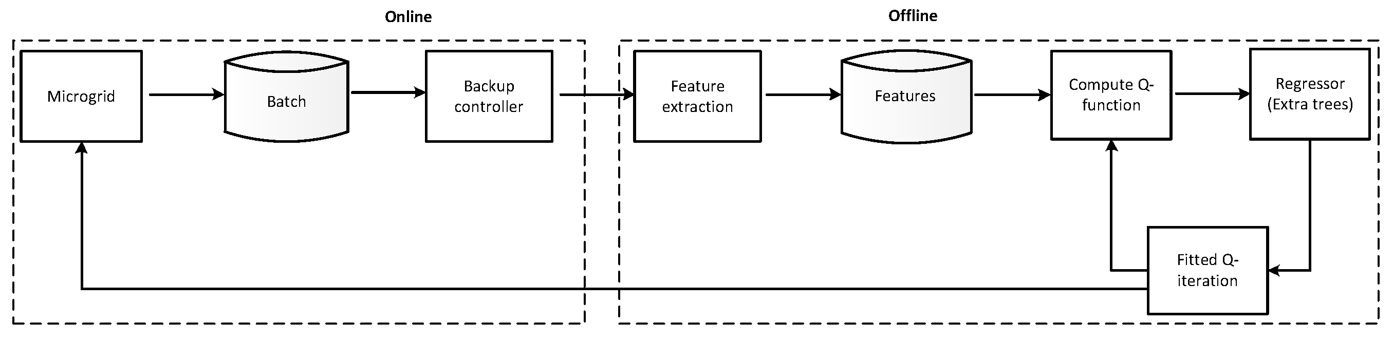
This section presents batch reinforcement learning, the fitted-Q iteration algorithm and the microgrid case study considered in this work. In model-free RL techniques, the learning agent does not require any prior information of the system. By interacting with the system, the agent collects new transitions that are added systematically to its batch, thus enriching its batch of experiences. The building blocks of batch RL are show in Figure 3.
4.1. Batch Reinforcement Learning
Batch RL is a branch of dynamic programming-based RL [30] and makes more efficient use of data and, thus, can achieve faster convergence to an optimal control policy compared to online RL techniques like Q-learning. In batch RL, a fixed batch of data is collected from the system a priori, and a control policy is learned from this batch of data. The goal of batch RL is to learn the best control policy from the given training data (batch) and use this policy on the environment. Thus, at the beginning of a control period, the learning agent uses a batch RL algorithm to construct a control policy, using a batch of past interactions with the system. In this paper, the proposed RL agent is applied to optimally schedule the operational mode of a battery in the microgrid described in Section 2. The observable state information contains input data on the state of the system. Before this information is sent to the batch RL algorithm, the learning agent can apply feature extraction. This feature extraction step selects only the state representation parameters necessary for the learning process.
The learning agent constructs a control policy that minimizes electricity cost, thus, since the load is not flexible in our setting, maximizing self-consumption of the locally-produced energy from the PV system and increasing the utilization rate of the battery. The solution of this control problem is a closed-loop control policy that is a function of the current state of the system. At every time step, a control action for the system is chosen according to Equation (9). This work uses the FQI algorithm to obtain a closed-loop policy from a batch of four-tuples containing the state, action, next state and corresponding cost (Equation (19)), where:
where is the next state and F the number of batches of tuples.
4.2. Fitted Q-Iteration
The FQI is one of the most popular batch RL algorithms. Fitted Q-iteration makes efficient use of gathered data samples and can be used together with any supervised learning method. In contrast to standard Q-learning , FQI computes the Q-function offline and makes use of the whole batch. Algorithm 1 presents an extended FQI algorithm that has been considered in this paper and in the work of Ruelens et al. [21]. The extension to the standard FQI comes in the form of a next state containing information on the forecasted uncontrollable exogenous component of the state space such as the load. This is in contrast with the standard FQI where the next state contains only past observations of the exogenous component. The algorithm iteratively constructs a training set () with all state-action pairs in as the input, as well as the targeted values consisting of the corresponding cost, Equation (18), and the optimal Q-values, Equation (7). The optimal Q-values are based on approximations of the Q-function from the previous iteration, for the next states and all actions, .
| Algorithm 1 Fitted Q-iteration with function approximation and forecast of exogenous information [21]. |
| Input: discount factor , control period T |
| 1: Generate samples |
| ← () observed exogenous component of the state is replaced by its forecast |
| 2: Initialize to zero for all state-action pairs, |
| 3: For do |
| 4: For do |
| 5: |
| 6: end for |
| 7: use a regression algorithm to build from |
| 8: end for |
| Output: |
In this work, a finite optimization horizon of T control periods is considered. The training set is constructed by iterating backwards over the training period. By considering this technique, the Q-function contains information about the future costs after one sweep over the training period. Thus, for the first iteration, , the Q-values in correspond to the immediate cost or revenue. For all other iterations, Q-values are calculated using the Q-function of the previous iteration. For all elements of the exogenous state space component, the successor state in is replaced by its forecast, . Thus, the next state contains information on the forecasted exogenous data. In the standard FQI [22] algorithm, the next state contains past observations of the exogenous data. By replacing the observed exogenous elements of the next state by their forecasts, the Q-function of the next state assumes that the exogenous information will follow its forecast, i.e., the Q-value of the next state becomes biased towards the provided forecast of the uncontrollable exogenous data. It is important to note that the operational planning of the battery is a continuous process in which the new SoC of the battery becomes the initial SoC in the next timestamp.
4.3. Regressor
Supervised learning algorithms can be used to build from the training set approximations of the Q-function, . Approximations of the Q-function are necessary to cope with the curse of dimensionality problem encountered when dealing with large or continuous state and/or action spaces [30]. Several types of function approximation techniques, such as neural network [34] and least-squares regression [35], can be used together with the FQI algorithm.
As a supervised learning method, this work considers a regression method based on an ensemble of extremely randomized trees (ExtRa-Trees) [36], to find an approximation of the Q-function. At every iteration k, a regressor function is constructed and used to build in the next iteration. A detailed overview of extremely randomized trees can be found in Geurts et al. [36]. ExtRa-Trees are robust (i.e., insignificantly affected by bad data and only in regions where the bad data are found) and have a fast computation time, which is the reason for their choice in this work.
4.4. Microgrid Case Study
The microgrid in this study is a single household consisting of: a battery of capacity 40 kWh with efficiency . The and of the battery are and , respectively. The battery discharge rate is fixed to 2 kW. We assume that the battery can absorb all energy produced by the PV system. Thus, there are no charge or discharge rate constraints. We consider an inverter of a capacity of 4 kW converting the DC power from the battery and PV to AC for the residential load and the grid. The inverter efficiency profile in Section 2.2, Figure 2, is considered. For the load and PV production profiles, we use data from the LINEAR (Local Intelligent Networks and Energy Active Regions) project [37]. The reader should note that this work focuses on the operational planning of the battery in the microgrid, and issues related to the real-time control aspects of the microgrid and the local utility grid to maintain frequency and voltage quality are out of the scope of this work.
The actions in can be represented in binary form with two contacts, S1 and S2 (0 = open, 1 = closed) for illustration, purposes as shown in Figure 4. This binary representation allows one to take into account the charge/discharge constraint, Equation (3). The binary representation of the actions is shown in Figure 4 and Table 1.
In this work, we consider that the battery can only be charged from the PV system as we focus on reducing the microgrid’s dependency on the external grid. However, in practical scenarios, it is also possible to charge the battery from the external grid during periods of low electricity prices.
5. Simulation Results and Discussion
This section presents the simulation results from four experiments and evaluates the performance of the proposed method using the indicators described in Section 5.3. In the first scenario, fixed electricity prices are considered, where . In the second scenario, the effect of dynamic electricity pricing on the control policy is investigated. In both scenarios, the battery’s SoC is uniformly sampled to 25 values in the interval [0,1]. The length of a control period is set to 15 min. The inverter nonlinearity, load uncertainty, battery constraints and the partial observability of the system form an important part of the environment, which the RL agent has to learn.
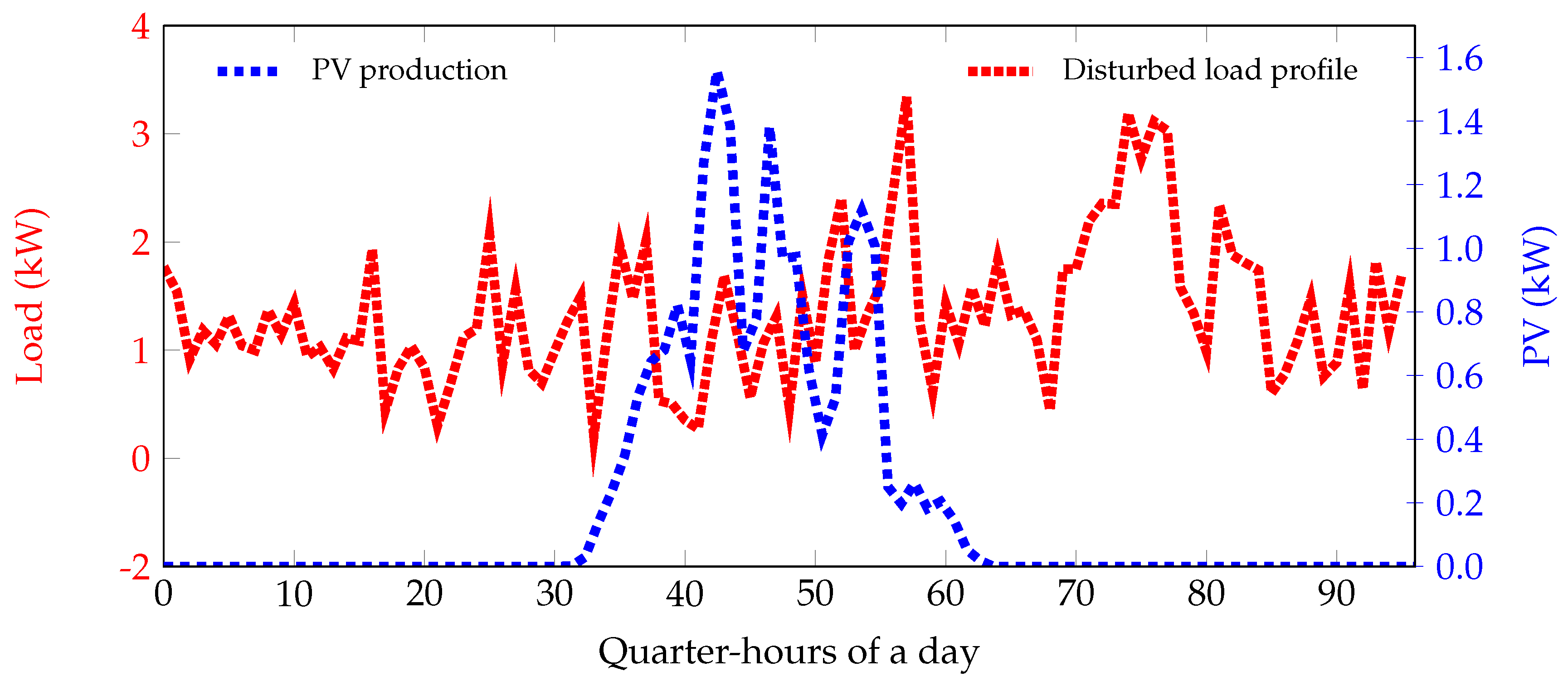
Figure 5 shows an example of the load and PV profiles over an optimization period of one day (96 quarter-hours) considered. Notice that, whatever the scenario, the agent ensures that the battery is always almost fully discharged to at the end of the control period in order to avoid energy wastage.
5.1. Scenario 1: Fixed Electricity Prices
This scenario considers fixed electricity pricing and has three experiments. The initial SoC of the battery is different in each experiment. This is to show that the approach can work for any initial battery SoC. The agent was trained for a period of one day.
- Experiment 1This experiment shows the policy obtained when the elements of the exogenous component of the state space are not considered, i.e., . A perfect forecast of the load and PV generation is provided. Simulation results are presented in Figure 6.
- Experiment 2In this experiment, all the elements of the exogenous component of the state space are considered. . The load and the PV are discretized to 50 discrete values between kW and kW, 0 kW and 8 kW respectively. Figure 7 shows the control policy and SoC evolution learned by the agent.
- Experiment 3The final experiment in this scenario considers that . A disturbance is added to the perfect load forecast to introduce uncertainty, as illustrated in Figure 8. This disturbance is white noise; standard normal distribution, i.e., a normal distribution with mean, , and standard deviation, . We choose to introduce a disturbance in the load because it is common in real life to have uncertainties in the energy usage patterns of residential consumers. Simulations results can be seen in Figure 9. By learning the time component of the feature space, the RL agent can learn the PV production profile. A perfect forecast of the PV generation is provided. The load is uniformly sampled to 50 values between kW and kW.
The solid blue line in Figure 10 presents an example of a control policy learned by the agent over a period of one day. The control policy represents the best actions that can be taken by the agent when the microgrid is in a particular state, over the state space. It can be seen from the policy that the agent discharges the battery during periods of little or no PV production depending on the battery SoC. During high production, the agent charges the battery, thus building up its reserve. During the first 30 quarter-hours of the day, the agent decides to keep the battery idle. This is because keeping the battery idle or charging the battery results in the same cost as there is no PV production. Notice that: (i) The agent sometimes decides to keep the battery idle during high PV production. This is because the PV produced is matching the demand. This is also because the agent avoids having some energy left in the battery at the end of the optimization period. Thus, this ensures that the battery is discharged to at the end of the optimization period. (ii) The agent decides to discharge the battery even in the presence of enough PV production. This can be explained as due to the influence of the inverter efficiency. The agent discharges the battery in order to achieve a higher inverter efficiency. All these decisions are made depending on the features in the state space and values of the Q-functions over the entire state space for every action.
The solid blue lines in Figure 6, Figure 7, Figure 8 and Figure 9 show examples of corrected control policies of the agent; corrected in the sense that the effect of the backup controller has been incorporated in the policy learned by the agent. Figure 6 represents the corrected control policy from Experiment 1. The agent requested to either discharge the battery or to keep the battery idle during the first 30 quarter-hours (Figure 10). However, due to the SoC of the battery (), the backup controller corrects this action by requesting for the battery to be discharged as the capacity constraint, Equation (2), is being violated. Notice that that sometimes a requested charge action from the backup controller has no effect on the SoC as there is no PV production at that instance, and this can be seen during the first 30 quarter-hours of Figure 7. This clearly shows the effect of the backup controller when the .
5.2. Scenario 2: Dynamic Electricity Pricing
In this scenario, a varying electricity price profile is considered. A sinusoidal price profile is chosen as shown in Figure 11. The price profile also considers periods when the price of buying electricity is less than the price of selling. This is a possible phenomenon in the real world especially in the imbalance market. Similar to Scenario 1, the control policy and SoC trajectory can be seen in Figure 12. This scenario shows the effect of varying electricity prices on the control policy. When the price of buying electricity is lower than the price of selling electricity, the agent decides to: (i) keep the battery idle and buy electricity from the grid (case of no PV production and ; period around the 20th quarter-hour of the day), (ii) charge the battery and buy electricity from the grid if (period around the 45th quarter-hour of the day, Figure 12) or (iii) discharge the battery in order to reduce the amount of energy bought from the grid, thus reducing electricity cost (period around the 70th quarter-hour of the day).
5.3. Performance Indicators
In this paper, the performance of the proposed RL controller is analyzed by considering the indicators discussed below.
- (a)
- Battery utilization rate, B: the ratio of the cumulative power from the PV used to charge the battery, described by the following equation.
- (b)
- Inverter power utilization rate, P:
- (c)
- Net electricity cost :where , .
The figures presented in Table 2 and Table 3 have been considered for an initial battery SoC of , over a period stretching from 1 January 2014–28 February 2014. An extract of PV generation and the consumption profile for a single day within this period can be seen in Figure 5. For Scenario 1, .
Table 2 shows the performance indicators for a microgrid with a single house in the case of fixed electricity prices, Scenario 1. The reader should note that the indicators of Experiment 3 have been considered for a standard deviation of in order to avoid large deviations from the deterministic setting. To analyze the performance, Experiment 1 will be used as the reference, i.e., the exogenous component of the state space is not considered. In Experiment 2, with the exogenous component of the state space considered, the battery utilization rate increases by , and the inverter power utilization rate increases by . This is reflected in the drop in the net electricity cost paid by the residential user. For Experiment 3, simulations were run five times and the average of the indicators taken. Comparing Experiment 3 with Experiment 1, i.e., by including the load feature in the state space with a disturbance, the battery utilization rate increases, but the inverter power utilization rate drops, an increase in net electricity cost can also be observed. This is because, as a result of the disturbance, a slight increase in the total demand is observed: kW as opposed to kW in Experiment 1.
This shows that, by including elements of the exogenous components in the feature space, the learning process of the agent is enhanced, and a better control policy is obtained.
Table 3 presents performance indicators in the case of dynamic electricity prices, i.e., Scenario 2. It is worth mentioning that the same experiments as in Scenario 1 are carried out, but for the introduction of dynamic prices. An increases in the battery utilization rate and a drop in the net electricity cost are observed compared to the experiments in Scenario 1. This is due to the possibility of having electricity prices lower than the fixed prices in Scenario 1.
5.4. Theoretical Benchmark in CPLEX
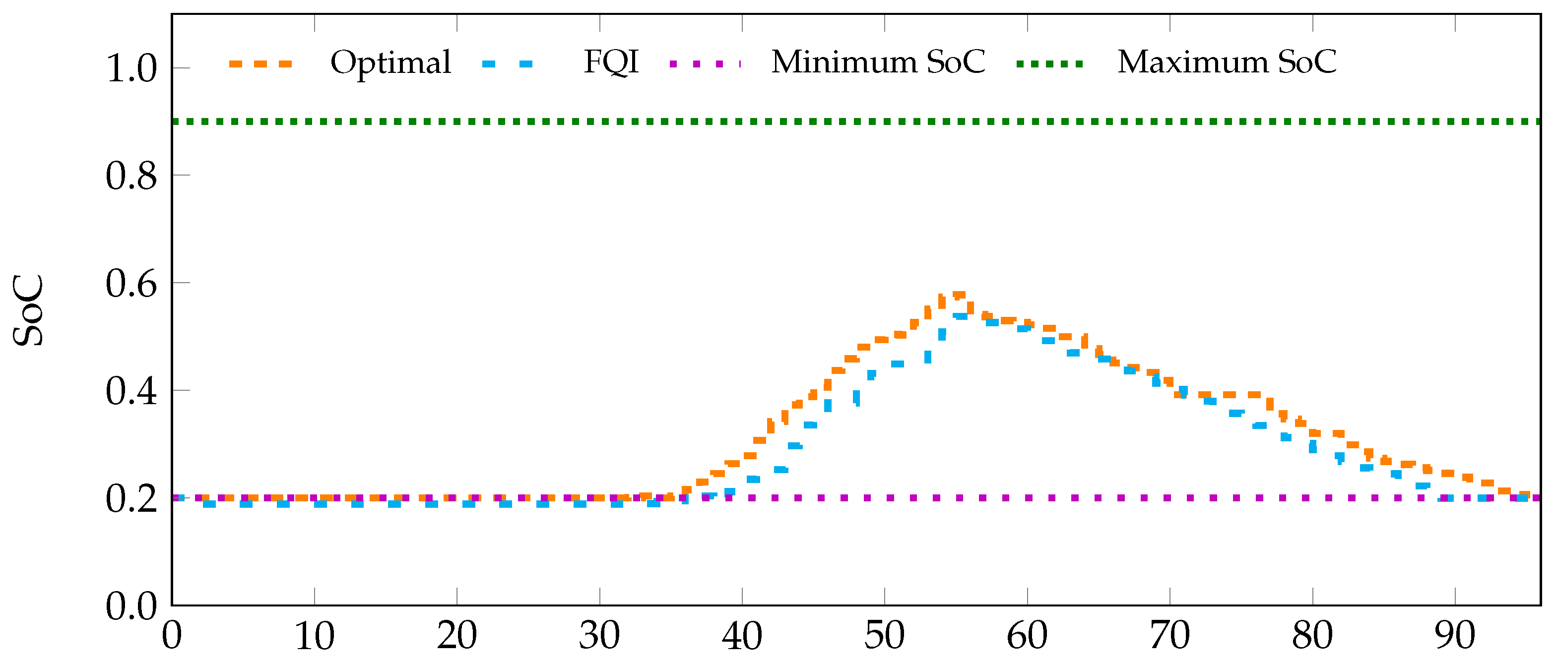
In order to see how well the proposed method behaves compared to other optimization techniques, an optimal controller was developed. This optimal controller is model-based and has full information about the microgrid. As such, a microgrid model was created containing information on all microgrid components and a perfect forecasts of all exogenous variables, i.e., the PV generation and load profiles. The optimal controller formalizes the problem as a mixed integer linear problem and uses CPLEX (OPL), a commercial optimization solver [38]. The settings of Scenario 1, Experiment 1 are considered. Simulation results showing the evolution of the battery’s SoC for an optimization period of 96 quarter-hours are depicted in Figure 13.
As shown in Figure 13, in the case of the optimal controller, the system constraints are perfectly respected, and there is no need for a backup controller. To clearly compare the two methods, the net electricity costs are considered, and a performance gap metric is used G:
A performance gap, G, of between extended FQI and the optimal controller was obtained. This shows that higher electricity costs are paid when the FQI algorithm is used. In model-based methods, model parameters are well defined, and an optimal solution is obtained based on this model and its parameters. The whole dataset is used to develop the model and obtain the optimal solution. As such, it is important to note that the same data that was used to compute the model parameters is used to evaluate the model. This is not an accurate evaluation of the model-based method, as this would require splitting the data into seperate training and test sets. However, it does provide a good benchmark / base line for the FQI algorithm, as it incorporates ‘future’ information not known at each point in the simulation. However, this performance is realistic as the microgrid model is unknown to the RL agent.
6. Conclusions and Future Work
This paper has presented a data-driven control approach applied to battery energy management in microgrids. Specifically, a model-free batch reinforcement learning technique, the extended fitted-Q iteration algorithm, has been used to control the operation mode of a battery storage device in a microgrid. The objective was to maximize self-consumption of the locally-produced energy from the PV system, hence minimizing the electricity cost and dependency on the local utility grid. The stochastic occupant behavior in the residential setting, the PV production profile and the nonlinearity from the inverter efficiency have been accounted for in the construction of a closed-loop control policy by the RL agent. The performance of the learning algorithm has been evaluated using three indicators. Simulation results showed that by including exogenous features on the feature space, the learning process was enhanced. However, the computation time increased significantly. Simulations were equally run with data from a summer period and similar results obtained. Encouraged by the values of the performance indicators, the proposed approach of batch RL can be up-scaled to a more realistic microgrid setting integrating more complex scenarios with constraints at the local utility grid level, battery charging and discharge rates and a continuous action space.
Future work will consider: (i) RL in a stochastic setting where the next state is conditioned by a probability density defined by the current state and action, (ii) the effect of load flexibility using heat pumps and domestic hot water storage on the control policy and (iii) the optimization potential in clusters of microgrids with completely different electricity usage patterns and limited communication capabilities between the microgrids.
Acknowledgments
The authors would like to thank the Vlaamse Instelling voor Technologisch Onderzoek (VITO) and the SmileIT (Stable MultI-agent LEarnIng for neTworks) project for funding this research.
Author Contributions
This paper is in partial fulfillment of the requirements of the doctoral research of Brida V. Mbuwir, supervised by Fred Spiessens and Geert Deconinck. All authors have been involved in the preparation of the manuscript.
Conflicts of Interest
The authors declare no conflict of interest.
Abbreviations
The following abbreviations are used in this manuscript:
| AC | Alternating Current |
| DC | Direct Current |
| FQI | Fitted-Q Iteration |
| MDP | Markov Decision Process |
| PV | Photovoltaic |
| RES | Renewable Energy Sources |
| RL | Reinforcement Learning |
| SoC | State of Charge |
References
- Voropai, N.I.; Efimov, D.N. Operation and control problems of power systems with distributed generation. In Proceedings of the 2009 IEEE Power Energy Society General Meeting, Calgary, AB, Canada, 26–30 July 2009; pp. 1–5. [Google Scholar]
- European Commission: Energy, Moving towards a Low Carbon Economy. Available online: https://ec.europa.eu/energy/en/topics/renewable-energy (accessed on 23 August, 2017).
- Leo, R.; Milton, R.S.; Sibi, S. Reinforcement learning for optimal energy management of a solar microgrid. In Proceedings of the Global Humanitarian Technology Conference—South Asia Satellite (GHTC-SAS), Trivandrum, India, 26–27 September 2014; pp. 183–188. [Google Scholar]
- Dimeas, A.L.; Hatziargyriou, N.D. Agent based Control for Microgrids. In Proceedings of the Power Engineering Society General Meeting, Tampa, FL, USA, 24–28 June 2007; pp. 1–5. [Google Scholar]
- Parhizi, S.; Lotfi, H.; Khodaei, A.; Bahramirad, S. State of the Art in Research on Microgrids: A Review. IEEE Access 2015, 3, 890–925. [Google Scholar] [CrossRef]
- François-Lavet, V.; Gemine, Q.; Ernst, D.; Fonteneau, R. Towards the minimization of the levelized energy costs of microgrids using both long-term and short-term storage devices. In Smart Grid: Networking, Data Management, and Business Models; CRC Press: Boca Raton, FL, USA, 2016; pp. 295–319. [Google Scholar]
- Zhao, B.; Xue, M.; Zhang, X.; Wang, C.; Zhao, J. An MAS based energy management system for a stand-alone microgrid at high altitude. Appl. Energy 2015, 143, 251–261. [Google Scholar] [CrossRef]
- Bacha, S.; Picault, D.; Burger, B.; Etxeberria-Otadui, I.; Martins, J. Photovoltaics in Microgrids: An Overview of Grid Integration and Energy Management Aspects. IEEE Ind. Electron. Mag. 2015, 9, 33–46. [Google Scholar] [CrossRef]
- Tesla Gigafactory. Available online: https://www.tesla.com/gigafactory (accessed on 4 July 2017).
- Van Moffaert, K.; De Hauwere, Y.M.; Vrancx, P.; Nowé, A. Reinforcement Learning for Energy-Reducing Start-Up Schemes. In Proceedings of the 24th Benelux Conference on Artificial Intelligence, Maastricht, The Netherlands, 25–26 October 2012. [Google Scholar]
- Camacho, E.F.; Alba, C.B. Model Predictive Control; Springer Science & Business Media: Berlin/Heidelberg, Germany, 2013. [Google Scholar]
- Ernst, D.; Glavic, M.; Capitanescu, F.; Wehenkel, L. Reinforcement learning versus model predictive control: A comparison on a power system problem. IEEE Trans. Syst. Man Cybern. Syst. 2009, 39, 517–529. [Google Scholar] [CrossRef] [PubMed]
- Bifaretti, S.; Cordiner, S.; Mulone, V.; Rocco, V.; Rossi, J.; Spagnolo, F. Grid-connected Microgrids to Support Renewable Energy Sources Penetration. Energy Procedia 2017, 105, 2910–2915. [Google Scholar] [CrossRef]
- Prodan, I.; Zio, E. A model predictive control framework for reliable microgrid energy management. Int. J. Electr. Power Energy Syst. 2014, 61, 399–409. [Google Scholar] [CrossRef]
- Bertsekas, D. Dynamic Programming and Optimal Control; Athena Scientific: Belmont, MA, USA, 1995. [Google Scholar]
- Costa, L.M.; Kariniotakis, G. A Stochastic Dynamic Programming Model for Optimal Use of Local Energy Resources in a Market Environment. In Proceedings of the 2007 IEEE Lausanne Power Tech, Lausanne, Switzerland, 1–5 July 2007; pp. 449–454. [Google Scholar]
- Sutton, R.S.; Barto, A.G. Reinforcement Learning: An Introduction; MIT Press: Cambridge, MA, USA, 1998. [Google Scholar]
- Kuznetsova, E.; Li, Y.F.; Ruiz, C.; Zio, E.; Ault, G.; Bell, K. Reinforcement learning for microgrid energy management. Energy 2013, 59, 133–146. [Google Scholar] [CrossRef]
- Dimeas, A.; Hatziargyriou, N. Multi-agent reinforcement learning for microgrids. In Proceedings of the Power and Energy Society General Meeting, Providence, RI, USA, 25–29 July 2010; pp. 1–8. [Google Scholar]
- Lee, D.; Powell, W. An Intelligent Battery Controller Using Bias-Corrected Q-learning. In Proceedings of the Twenty-Sixth AAAI Conference on Artificial Intelligence, Toronto, ON, Canada, 22–26 July 2012. [Google Scholar]
- Ruelens, F.; Claessens, B.; Vandael, S.; De Schutter, B.; Babuska, R.; Belmans, R. Residential demand response applications using batch reinforcement learning. arXiv, 2015; arXiv:1504.02125. [Google Scholar]
- Ernst, D.; Geurts, P.; Wehenkel, L. Tree-based batch mode reinforcement learning. J. Mach. Learn. Res. 2005, 6, 503–556. [Google Scholar]
- Lange, S.; Gabel, T.; Riedmiller, M. Reinforcement learning: State-of-the-Art. Springer 2012, 12, 45–73. [Google Scholar]
- Ruelens, F.; Iacovella, S.; Claessens, B.J.; Belmans, R. Learning agent for a heat-pump thermostat with a set-back strategy using model-free reinforcement learning. Energies 2015, 8, 8300–8318. [Google Scholar] [CrossRef]
- Claessens, B.J.; Vandael, S.; Ruelens, F.; De Craemer, K.; Beusen, B. Peak shaving of a heterogeneous cluster of residential flexibility carriers using reinforcement learning. In Proceedings of the 2013 4th IEEE/PES Innovative Smart Grid Technologies Europe (ISGT EUROPE), Lyngby, Denmark, 6–9 October 2013; pp. 1–5. [Google Scholar]
- Ruelens, F.; Claessens, B.J.; Vandael, S.; Iacovella, S.; Vingerhoets, P.; Belmans, R. Demand response of a heterogeneous cluster of electric water heaters using batch reinforcement learning. In Proceedings of the Power Systems Computation Conference (PSCC), Wroclaw, Poland, 18–22 August 2014; pp. 1–7. [Google Scholar]
- Vandael, S.; Claessens, B.; Ernst, D.; Holvoet, T.; Deconinck, G. Reinforcement learning of heuristic EV fleet charging in a day-ahead electricity market. IEEE Trans. Smart Grid 2015, 6, 1795–1805. [Google Scholar] [CrossRef]
- De Somer, O.; Soares, A.; Kuijpers, T.; Vossen, K.; Vanthournout, K.; Spiessens, F. Using Reinforcement Learning for Demand Response of Domestic Hot Water Buffers: A Real-Life Demonstration. arXiv, 2017; arXiv:1703.05486. [Google Scholar]
- François-Lavet, V.; Taralla, D.; Ernst, D.; Fonteneau, R. Deep reinforcement learning solutions for energy microgrids management. In Proceedings of the European Workshop on Reinforcement Learning (EWRL 2016), Barcelona, Spain, 3–4 December 2016. [Google Scholar]
- Busoniu, L.; Babuška, R.; De Schutter, B.; Ernst, D. Reinforcement Learning and Dynamic Programming Using Function Approximators; CRC Press: Boca Raton, FL, USA, 2010. [Google Scholar]
- Ernst, D.; Glavic, M.; Geurts, P.; Wehenkel, L. Approximate Value Iteration in the Reinforcement Learning Context. Application to Electrical Power System Control. Int. J. Emerg. Electr. Power Syst. 2005, 3. [Google Scholar] [CrossRef]
- Olivares, D.E.; Mehrizi-Sani, A.; Etemadi, A.H.; Cañizares, C.A.; Iravani, R.; Kazerani, M.; Hajimiragha, A.H.; Gomis-Bellmunt, O.; Saeedifard, M.; Palma-Behnke, R.; et al. Trends in Microgrid Control. IEEE Trans. Smart Grid 2014, 5, 1905–1919. [Google Scholar] [CrossRef]
- Driesse, A.; Jain, P.; Harrison, S. Beyond the curves: Modeling the electrical efficiency of photovoltaic inverters. In Proceedings of the 33rd IEEE Photovoltaic Specialists Conference, San Diego, CA, USA, 11–16 May 2008; pp. 1–6. [Google Scholar]
- Riedmiller, M. Neural fitted Q-iteration—First experiences with a data efficient neural reinforcement learning method. In Proceedings of the 16th European Conference on Machine Learning (ECML), Porto, Portugal, 3–7 October 2005; Springer: New York, NY, USA, 2005; Volume 3720, p. 317. [Google Scholar]
- Farahmand, A.M.; Ghavamzadeh, M.; Szepesvari, C.; Mannor, S. Regularized Fitted Q-Iteration for planning in continuous-space Markovian decision problems. In Proceedings of the 2009 American Control Conference, St. Louis, MO, USA, 10–12 June 2009; pp. 725–730. [Google Scholar]
- Geurts, P.; Ernst, D.; Wehenkel, L. Extremely randomized trees. Mach. Learn. 2006, 63, 3–42. [Google Scholar] [CrossRef]
- Linear Project. Available online: http://www.linear-smartgrid.be/en/research-smart-grids (accessed on 1 August 2017).
- ILOG, Inc. ILOG CPLEX: High-Performance Software for Mathematical Programming and Optimization, 2006. Available online: http://www.ilog.com/products/cplex/ (accessed on 14 September 2017 ).
Figure 1.
Microgrid architecture including DC/AC converters, to interface storage and generation to the load and the local utility grid.
Figure 1.
Microgrid architecture including DC/AC converters, to interface storage and generation to the load and the local utility grid.

Figure 2.
Efficiency curve of a 4 kW inverter extracted from [33].
Figure 2.
Efficiency curve of a 4 kW inverter extracted from [33].

Figure 3.
Building blocks of the batch reinforcement learning approach applied in a microgrid setting.
Figure 3.
Building blocks of the batch reinforcement learning approach applied in a microgrid setting.

Figure 4.
Energy flows within the microgrid with respect to the control actions.

Figure 5.
Load and PV profiles over a period of one day (96 quarter-hours).

Figure 6.
Scenario 1, Experiment 1: Corrected control policy of the agent and SoC trajectory. The yellow area shows the normalized PV production.
Figure 6.
Scenario 1, Experiment 1: Corrected control policy of the agent and SoC trajectory. The yellow area shows the normalized PV production.

Figure 7.
Scenario 1, Experiment 2: Corrected control policy of the agent and SoC trajectory. The yellow area shows the normalized PV production.
Figure 7.
Scenario 1, Experiment 2: Corrected control policy of the agent and SoC trajectory. The yellow area shows the normalized PV production.

Figure 8.
Scenario 1, Experiment 3: Load profile with white noise.

Figure 9.
Scenario 1, Experiment 3: Corrected control policy of the agent and SoC trajectory. The yellow area shows the normalized PV production.
Figure 9.
Scenario 1, Experiment 3: Corrected control policy of the agent and SoC trajectory. The yellow area shows the normalized PV production.

Figure 10.
Scenario 1, Experiment 1: Control policy learned by the agent and SoC trajectory. The yellow area shows the normalized PV production.
Figure 10.
Scenario 1, Experiment 1: Control policy learned by the agent and SoC trajectory. The yellow area shows the normalized PV production.

Figure 11.
Scenario 2, electricity price profiles.

Figure 12.
Scenario 2, Experiment 1: Corrected control policy of the agent and SoC trajectory. The yellow area shows the normalized PV production.
Figure 12.
Scenario 2, Experiment 1: Corrected control policy of the agent and SoC trajectory. The yellow area shows the normalized PV production.

Figure 13.
Simulation results with a fixed pricing scheme using an optimal controller (Optimal) and extended FQI (FQI). The plot depicts the SoC trajectory obtained for the two methods.
Figure 13.
Simulation results with a fixed pricing scheme using an optimal controller (Optimal) and extended FQI (FQI). The plot depicts the SoC trajectory obtained for the two methods.


Table 1.
Binary representation of control actions.
| Binary Representation | Action |
|---|---|
| 00: S1 = 0, S2 = 0 | Idle |
| 10: S1 = 1, S2 = 0 | Charge |
| 01: S1 = 0, S2 = 1 | Discharge |
| 11: S1 = 0, S2 = 1 | Not possible due to charge/discharge constraint, Equation (3) |
Table 2.
Scenario 1: performance indicators for the different scenarios during winter: January 2014–February 2014.
Table 2.
Scenario 1: performance indicators for the different scenarios during winter: January 2014–February 2014.
| Indicator | Experiment 1 | Experiment 2 | Experiment 3 |
|---|---|---|---|
| Battery utilization rate, | 27 | 47 | 32 |
| Inverter power utilization rate, | 17 | 21 | 17 |
| Net electricity cost, (euros) | 155 | 149 | 156 |
Table 3.
Scenario 2: performance indicators for the different scenarios during winter: January 2014–February 2014.
Table 3.
Scenario 2: performance indicators for the different scenarios during winter: January 2014–February 2014.
| Indicator | Experiment 1 | Experiment 2 | Experiment 3 |
|---|---|---|---|
| Battery utilization rate, | 30 | 49 | 34 |
| Inverter power utilization rate, | 18 | 21 | 17 |
| Net electricity cost, (euros) | 75 | 71 | 77 |
© 2017 by the authors. Licensee MDPI, Basel, Switzerland. This article is an open access article distributed under the terms and conditions of the Creative Commons Attribution (CC BY) license (http://creativecommons.org/licenses/by/4.0/).
Share and Cite
MDPI and ACS Style
Mbuwir, B.V.; Ruelens, F.; Spiessens, F.; Deconinck, G. Battery Energy Management in a Microgrid Using Batch Reinforcement Learning. Energies 2017, 10, 1846. https://doi.org/10.3390/en10111846
AMA Style
Mbuwir BV, Ruelens F, Spiessens F, Deconinck G. Battery Energy Management in a Microgrid Using Batch Reinforcement Learning. Energies. 2017; 10(11):1846. https://doi.org/10.3390/en10111846
Chicago/Turabian StyleMbuwir, Brida V., Frederik Ruelens, Fred Spiessens, and Geert Deconinck. 2017. "Battery Energy Management in a Microgrid Using Batch Reinforcement Learning" Energies 10, no. 11: 1846. https://doi.org/10.3390/en10111846
Note that from the first issue of 2016, this journal uses article numbers instead of page numbers. See further details here.