Online Area Load Modeling in Power Systems Using Enhanced Reinforcement Learning

Abstract

The accuracy of load modeling directly influences power system operation and control. Previous modeling studies have mainly concentrated on the loads connected to a single boundary bus, without thoroughly considering the static load characteristics of the voltage. To remedy this oversight, this paper proposes an accurate modeling approach for area loads with multiple boundary buses and ZIP loads (a combination of constant-impedance, constant-current and constant-power loads) based on Ward equivalence. Furthermore, to satisfy the requirements for real-time monitoring, the model parameters are identified in an online manner using an enhanced reinforcement learning (ERL) algorithm. Parallel tables of value functions are implemented in the ERL algorithm to improve its tracking performance. Three simulation cases are addressed, the first involving a single ZIP load and the second and third involving area loads in the IEEE 57-bus system and in a real 1209-bus power system in China, respectively. The results demonstrate that the ERL algorithm outperforms an existing reinforcement learning algorithm and the improved least-squares method in terms of convergence and the ability to track both step-changing and time-varying loads. Additionally, the results obtained on test cases confirm that the proposed area load model is more accurate than a previously introduced model.

1. Introduction

The expansion of power grids has significantly increased the complexity of power flow analysis, posing challenges for online dispatch and control. As a vital element of power flow analysis, load modeling has attracted extensive attention from researchers for decades. An ‘area load’ represents a specific load area network in a system, including its internal buses and devices [1]. When constructing a model of an area load, the aim is to simplify the topological structure of the power grid to decrease the computational burden of power flow analysis.

Load models can be classified into static and dynamic models [2]. Static models express the active and reactive power at any instant of time as functions of the bus voltage magnitudes and frequencies, which are typically in a steady state. The static load features of the area loads seen from a single boundary bus can be represented by a ZIP load (a combination of constant-impedance, constant-current and constant-power load) model [3] or by an exponential model [4]. A number of researchers has proposed static load models for area loads in distribution networks [5,6]. In reality, to ensure a reliable supply of power, electricity is delivered from external power supply networks to area loads through multiple lines simultaneously. Therefore, it is necessary to investigate an area load model with multiple boundary buses.

The first step of load modeling is to determine the model structure. Ward equivalence [7] is a classic approach for reducing the topological structure of area loads with multiple boundary buses for applications such as state estimation [8], security analysis [9] and network reconfiguration [10]. The equivalent system with $N+1$ buses proposed in paper [11] is an extension of the Thevenin equivalence approach combined with Ward equivalence, in which the equivalent loads are treated using a constant-impedance model. Our previous studies reported in [1,12] introduced another approach to area load modeling, which focuses on replacing the internal buses and lines with only one fictitious load bus and several fictitious lines linking that load bus to multiple boundary buses. A ZIP model is connected to the fictitious load bus to describe the load features of the area load in the form of internal ZIP loads.

The next step of load modeling is to identify the model parameters. Using synchronized phasor measurement units (PMUs), researchers can conveniently collect measurements at the boundary buses to derive the load characteristics. In reality, the system loads vary in time and thus cannot be simply treated as constants or ZIP loads with fixed coefficients, as is done in offline modeling approaches [13]. Moreover, it is difficult for the operators of transmission grids to obtain real-time information on the internal loads of distribution networks to serve as a basis for making operational decisions. Hence, an alternative approach is to optimize the model parameters online based on a sliding time window using real-time measurements at the boundary buses.

To achieve online optimization of the parameters of an area load model with a single boundary bus, papers [3,14] utilize a recursive least-squares (LS) method to minimize the error between the modeled and true area loads in each time window. LS methods are also widely used in other applications, such as the short-term forecasting of wind power [15], power estimation for electric vehicles [16], the design of filters [17], and the forecasting of electricity prices [18,19,20]. According to paper [11], the optimization problem corresponding to the modeling of an area load with multiple boundary buses is a complex non-linear programming problem with multiple local optima. In that paper, a sequential quadratic programming (SQP) method with improved initial points is used to optimize the parameters. Meanwhile, several assumptions are adopted to weaken the correlations among the model parameters, which can impair the accuracy of the model. Without these assumptions, more global optimization algorithms would be needed to solve the multi-mode optimization problem.

In applications involving the online control or dispatch of power systems, reinforcement learning (RL) methods have exhibited remarkable capabilities for performing online calculations [21,22,23]. RL is based on the concept of trial and error and explicitly considers the problem of a goal-directed agent interacting with an uncertain environment [24]. It originated in the study of animal intelligence [25] and has become a major branch of machine learning [26]. RL encompasses numerous learning mechanisms, and various optimization algorithms have been developed on the basis of these mechanisms. The method of function optimization by reinforcement learning (FORL) proposed in paper [27] was developed based on the idea of temporal-difference learning [24]. Evaluations of the FORL method on benchmark functions have demonstrated that it exhibits superior performance compared with most prevailing population-based algorithms in terms of both accuracy and convergence, especially in the case of multi-mode functions. The distinct advantage of the FORL method is that it involves a complementary operation related to covariance matrix adaptation [28], which enables the algorithm to solve optimization problems with a continuous domain. Several decentralized Q-learning algorithms have been proposed to eliminate the curse of dimensionality in traditional Q-learning. Additionally, a hysteretic Q-learning method [29] has been presented that considers both cooperation and coordination among agents by means of adaptive learning rates.

The two main contributions of this paper can be summarized as follows. (1) We propose a Ward equivalent model for area loads with multiple boundary buses. Unlike previous proposals, the model includes internal ZIP loads. (2) We develop an enhanced reinforcement learning (ERL) algorithm for identifying the model parameters based on real-time synchronized measurements taken at the boundary buses. Compared with the FORL method, two improvements are incorporated into the ERL algorithm, i.e., adaptive learning rates and parallel tables of value functions, to enhance its ability to track load changes quickly and accurately. Moreover, unlike the Q-learning algorithms mentioned above, the ERL algorithm can be used to solve the parameter identification problem with a continuous solution domain.

The remainder of the paper is organized as follows. In Section 2, the Ward equivalent model is presented. The ERL algorithm is introduced in Section 3. Simulation studies are reported in Section 4. In the final section, conclusions are drawn, and future work is discussed.

2. Area Load Modeling and Topological Structure Simplification of Power Systems

Electric power is delivered from a power supply network to an area load through boundary buses. Consider the IEEE 57-bus power system, for example. Figure 1a illustrates the 57-bus power system, in which the area load to be simplified includes 11 branches and eight buses. The loads included in the area load are ZIP loads. Suppose that synchronized PMUs are configured on boundary buses 22, 29 and 32; thus, the voltage phasors ${\dot{V}}_i(i=1,2,3)$ at these boundary buses and the current phasors ${\dot{I}}_i(i=1,2,3)$ injected into the area load can be measured accordingly.

In the conventional Ward equivalence approach, the internal buses in the area load are simplified as fictitious lines between each pair of boundary buses. The resulting Ward equivalent model is depicted in Figure 1b. The model parameters include the admittances of the fictitious lines, $g_{ij}$ and $b_{ij}(i,j=1,2,3\mathrm{and}i\ne j)$, and the fictitious load parameters. The fictitious loads in conventional Ward equivalent models are constant-current or constant-power loads; therefore, the nodal admittance matrix (or the parameters) of the equivalent model can be determined by performing Gaussian elimination on the nodal admittance matrix of the area load. Paper [11] treats these loads as constant impedances, and the model parameters are determined using measurements collected at the boundary buses. In this paper, the accuracy of the model is improved by formulating ZIP models of the active and reactive loads as follows [30]:

$$\left\{\begin{array}{c}\hfill P_i=a_{\mathrm{p}i,1}{V}_i^2+a_{\mathrm{p}i,2}{V}_i+a_{\mathrm{p}i,3}\\ \hfill Q_i=a_{\mathrm{q}i,1}{V}_i^2+a_{\mathrm{q}i,2}{V}_i+a_{\mathrm{q}i,3}\end{array}\right.$$

(1)

where $a_{\mathrm{p}i,j}$ and $a_{\mathrm{q}i,j}(i,j=1,2,3)$ are load coefficients. All parameters in the proposed model are estimated through online training based on real-time measurements to ensure that the model parameters are kept up to date to track the time-varying loads.

3. The Enhanced Reinforcement Learning Algorithm for Online Parameter Tracking

In this section, an ERL algorithm is proposed for identifying the parameters of the area load model. An overview is first presented to introduce the basic procedures of RL. A flowchart is also included to illustrate the implementation of the proposed algorithm for the online tracking of the model parameters. The main steps of the ERL algorithm are then described in detail.

3.1. Overview

In an RL algorithm, agents first sense the current state of the environment. They are not told which actions to take; instead, they must discover which actions yield the greatest reward generated by the environment [24]. In turn, the behavior of the agents causes the environment to transition into a new state. In this way, actions that result in good or bad outcomes have a tendency to be reselected or abandoned, respectively.

The basic elements of the ERL algorithm are defined below. Suppose that the proposed model contains N parameters; thus, the control variables for parameter identification can be denoted by $Z=[z_1,z_2,\cdots ,z_N]$. Accordingly, N agents are employed, each of which is responsible for one control variable. The feasible domain of the i-th dimension of Z is then discretized into $D_i$ cells. Thus, the action set of agent i can be denoted by $A_i=\{1,2,\cdots ,D_i\}(i=1,\cdots ,N)$. When agent i takes its j-th action, this indicates that the corresponding one-dimensional control variable will be randomly chosen from the corresponding cell. In the ERL algorithm, the environment state refers to the accuracy of the model, which is quantified as the value of an error function, $F\left(Z\right)$. Instead of calculating values for ‘state-action’ pairs, as in the case of conventional RL algorithms, the ERL algorithm only records value functions for actions. For instance, the value function of the j-th action conducted by the i-th agent is denoted by $\mathcal{Q}(i,j)$. These value functions are updated by means of a scalar reward R, which is generated by the environment.

The online parameter tracking process that is implemented by means of the ERL algorithm is depicted in Figure 2. The learning behavior of the agents is shown in the dashed box, and the four main steps of this behavior are described in detail in Section 3.2, Section 3.3, Section 3.4 and Section 3.5 below. First, an agent evaluates the current solution based on voltage and current measurements, after initialization of the counter k. Note that in this paper, the measurements have been filtered to remove noise before parameter identification. A scale reward or punishment signal (one or $-1$) is then fed back to the agent, indicating whether the selected action is beneficial or not, respectively. Meanwhile, the best solution $Z_{\mathrm{best}}$ is updated and sent to the area load model. The value function is then updated with the immediate reward. The agent then selects a new action from its action set based on the updated value functions. The counter is increased by one every time an agent completes the above cycle of learning behavior. Agents take turns repeating this learning cycle until the counter reaches a preset threshold, $k_{\max }$. Similar to the FORL procedure presented in [27], once agent N completes its learning behavior, different tiny perturbations are simultaneously applied to all of the one-dimensional solutions. This complementary operation facilitates the full exploitation of favorable actions.

Compared with the FORL method proposed in [27], which has shown excellent optimization performance on high-dimensional and multi-modal functions, the ERL algorithm includes two improvements concerning the updating of the value functions. First, adaptive learning rates, which were first used in [29], are adopted for the agents to allow them to exhibit cooperation and coordination behaviors. Second, parallel tables of value functions are introduced to accumulate the search experience gained under different load demands.

3.2. State Evaluation

The area load model is trained under the same voltages as in the original area load. The voltage measurements ${\dot{V}}^{\mathrm{m}}$ are imposed on the model, and the currents ${\dot{I}}_1^{\mathrm{c}}\sim {\dot{I}}_n^{\mathrm{c}}$ flowing from the boundary buses to the model are calculated. The environment state is then evaluated by calculating the root-mean-square error between the calculated currents (${\dot{I}}_1^{\mathrm{c}}\sim {\dot{I}}_n^{\mathrm{c}}$) and the measured currents (${\dot{I}}_1^{\mathrm{m}}\sim {\dot{I}}_n^{\mathrm{m}}$), which is formulated as the following error function:

$$F\left(Z\right)=\sqrt{1/n_{\mathrm{s}}{\sum }_{s=1}^{n_{\mathrm{s}}}{\sum }_{i=1}^n{\left(\mid {\dot{I}}_{i,s}^{\mathrm{m}}-{\dot{I}}_{i,s}^{\mathrm{c}}\left(Z\right)\mid /\mid {\dot{I}}_{i,s}^{\mathrm{m}}\mid \right)}^2}$$

(2)

where $n_{\mathrm{s}}$ is the number of samples. The value of this function reflects the accuracy of the optimized model in each sliding time window, which is frequently used as the objective function for parameter identification [31,32,33]. Given ${\dot{V}}^{\mathrm{m}}$, ${\dot{I}}_{i,s}^{\mathrm{c}}\left(Z\right)$ is calculated based on the current solution Z in accordance with the circuit shown in Figure 1b.

3.3. Reward Calculation

Once an agent relocates within its own dimension, it obtains a signal indicating whether the area load model with the current parameters is more accurate than the model with the previous parameters. Based on a combined evaluation of the current locations of all agents, $Z^{k+1}$, a reward or punishment signal is generated according to the following rule:

$$R=\left\{\begin{array}{cc}1\hfill & \mathrm{if}F\left(Z^{k+1}\right)\le F\left(Z_{\mathrm{best}}\right)\hfill \\ -1\hfill & \mathrm{otherwise}\hfill \end{array}\right.$$

(3)

where $Z_{\mathrm{best}}$ is currently the best solution that has been found based on the same samples, and this signal is then used in the learning process to update the value function. A positive signal will increase the value of the current action, and vice versa, as expressed in (4) and (5).

3.4. Value Function Update

3.4.1. Decentralized Strategy

The ERL algorithm uses a decentralized strategy [34] to update the value functions. The value function of the j-th action taken by the i-th agent is updated as follows:

$$\begin{array}{c}\hfill {\mathcal{Q}}^{k+1}(i,j)=(1-\alpha ){\mathcal{Q}}^k(i,j)+\alpha \left(R+\gamma \underset{j}{max}{\mathcal{Q}}^k(i,j)\right)\\ \hfill (i=1,2,\cdots ,N\mathrm{and}j=1,2,\cdots ,D_i)\end{array}$$

(4)

where $\alpha$ is the learning rate and $\gamma$ is the discount factor. In this decentralized strategy, agent i accumulates its own value functions without knowledge of the actions taken by other agents.

The value functions considered in the ERL algorithm are illustrated in

Table 1. $\mathcal{Q}$-table used in the decentralized strategy.

	Action	1	2	⋯	$$\begin{gathered} \begin{array}{c}\hfill {\mathit{D}}_{\mathit{i}} \\ (\mathit{i}=1,2,\cdots ,\mathit{N})\end{array} \end{gathered}$$
Agent
1		$\mathcal{Q}(1,1)$	$\mathcal{Q}(1,2)$	⋯	$\mathcal{Q}(1,D_1)$
2		$\mathcal{Q}(2,1)$	$\mathcal{Q}(2,2)$	⋯	$\mathcal{Q}(2,D_2)$
⋮		⋮	⋮	⋱	⋮
N		$\mathcal{Q}(N,1)$	$\mathcal{Q}(N,2)$	⋯	$\mathcal{Q}(N,D_N)$

. When agent i takes action $j(j\in A_i)$, the element $\mathcal{Q}(i,j)$ in row i and column j is updated. Agents take turns updating elements in their own rows. The values of all elements in the table are initialized as zero. Therefore, in each row, given proper $\alpha$ and $\gamma$ values, the values of the value functions that correspond to more favorable actions are larger. In turn, these favorable actions will be selected more frequently. Note that despite adopting a decentralized update strategy, the ERL algorithm does not optimize the model parameters independently, since the reward is determined based on the values of all parameters.

3.4.2. Adaptive Learning Rates

The ERL algorithm employs adaptive learning rates [29]. Consequently, the update rule for the value function of the j-th action taken by the i-th agent is rewritten as follows:

$$\delta \left(i\right)=R+\gamma \underset{j}{max}{\mathcal{Q}}^k(i,j)-{\mathcal{Q}}^k(i,j)$$

(5)

$${\mathcal{Q}}^{k+1}(i,j)=\left\{\begin{array}{cc}{\mathcal{Q}}^k(i,j)+\alpha \delta \left(i\right)\hfill & \mathrm{if}\delta \left(i\right)\ge 0\hfill \\ {\mathcal{Q}}^k(i,j)+\beta \delta \left(i\right)\hfill & \mathrm{otherwise}\hfill \end{array}\right.$$

(6)

where $\alpha$ and $\beta$ are the learning rates for increasing and decreasing the value function, respectively, and $1>\alpha >\beta >0$. When the increment $\delta \left(i\right)$ is positive, the estimated joint solution is currently the best. Thus, all agents have taken favorable actions that should be encouraged. By contrast, when $\delta \left(i\right)$ is negative, all agents have taken potentially adverse actions. In this case, it is difficult to determine whether the current action should be punished, so a low learning rate is suitable. If not, a high learning rate may decrease the probability of selecting this favorable action, preventing the model parameter optimized by this agent from reaching its optimal value. Considering these two cases, adaptive learning rates are utilized for updating the value function of the current action. A high learning rate $\alpha$ can increase the value of a favorable action, thereby enhancing its possibility of being selected. Meanwhile, when an adverse solution occurs (when $\delta \left(i\right)<0$), a relatively low learning rate $\beta$ is suitable for imposing only a slight punishment for the current action.

3.4.3. Parallel Tables

The measurement values are influenced by the load rate of the area load, which is defined as the ratio of the current load demand to the maximal load demand of the area load. In practice, the load demand or load rate is typically varying in time, as in the consumption profiles presented in paper [2]. Figure 3 shows the profile for the summer residential class, where the vertical coordinate represents the load rate. Under different load rates, the area load model requires different parameters. Therefore, as the load rate varies dramatically throughout the day, the favorable actions of agents should also change accordingly.

The ERL algorithm uses multiple tables of value functions to assign high values to different actions that are favorable under different load rates. For example, in Figure 3, the load rate values are evenly partitioned into several intervals, with the partition points denoted by $P_1$, $P_2$ and $P_3$. Accordingly, the same number of $\mathcal{Q}$-tables is utilized to store the value functions corresponding to each load rate interval. The ERL algorithm identifies the interval in which the current load rate of the load area network lies and then updates the value functions in the corresponding table. We suggest that the number of intervals should be no more than three; otherwise, the tables cannot be fully explored.

3.5. Action Selection

Each agent selects its action based on the values in its row of the $\mathcal{Q}$-table. More specifically, starting from the j-th element of the i-th row in Table 1, agent i can move either leftwards or rightwards to select the next action on the left or right path, respectively. Each path has a path value $L_l(i,j)(l=1,2)$, which is used to estimate the potential to find a better one-dimensional solution along that path. The selection probabilities for the paths, $p_1\left(l\right)(l=1,2)$, are determined by the path values. Along the selected path, agent i then chooses its next action from among the g adjacent actions according to their action probabilities, $p_2\left(h\right)(h=1,2,\cdots ,g)$. The formulations of the path values, path probabilities and action probabilities can be found in [27].

4. Case Studies

In this section, three simulation cases are presented to demonstrate the advantages of the ERL algorithm in comparison with the LS and FORL algorithms. Subsequently, the accuracy of the optimized models is examined in non-base scenarios. The presented analyses are summarized in

Table 2. Summary of the analyses.

Section	Analyses
4.1.1	A single ZIP load with stepwise changes
4.1.2	A time-variant Ward equivalent model in the IEEE 57-bus power system
4.1.3	A time-variant Ward equivalent model in a real 1209-bus power system
4.2.1	Accuracy verification for the ERL algorithm
4.2.2	Accuracy comparison among the ERL, FORL and LS algorithms
4.2.3	Accuracy comparison between the Ward equivalent model and the model from [35]

.

4.1. Online Tracking of Area Load Parameters

The first case, described in Section 4.1.1, involves a single ZIP load and is investigated to examine the performance of the ERL algorithm when tracking load coefficients exhibiting stepwise changes. In the next case, described in Section 4.1.2, the algorithms are utilized to track the time-varying parameters of the Ward equivalent model presented in Figure 1b in order to demonstrate the continuous optimization capability of the ERL algorithm in a time-varying system. Since the actual parameters of the model are unknown, the objective function values obtained by the algorithms are presented as indicators of the accuracy of the optimized models. A real 1209-bus power system from China is then employed to examine the proposed modeling approach, and the case is described in Section 4.1.3.

4.1.1. Single ZIP Load

This case demonstrates the performance of the ERL algorithm on a single ZIP load connected to a load bus. Time-varying voltage signals are imposed on the load bus, and current measurements are collected at the load bus. The ERL, FORL and LS algorithms are used to optimize the coefficients of the ZIP load in accordance with the real-time voltage measurements. As is done in [11], the initial values in the current time window are set to the optimal values for the last time window in the LS algorithm. The parameters of the ERL algorithm are set as follows: $D_i=10(i=1,2,\cdots ,N)$, $\alpha =0.5$, $\beta =0.1$ and $\gamma =0.9$. The value of $D_i$ is determined by referring to [27], and the values of $\alpha ,\beta$ and $\gamma$ are suggested in [29]. The parameters of the FORL algorithm are set equal to those in [27]. The sampling rate of the synchronized PMUs is 1 Hz. The ERL and FORL algorithms both perform 200 objective function evaluations at a frequency of 1 Hz using the measurements from the most recent ten-second time window. The LS algorithm uses the same time window and operates at the same frequency. The total simulation period is 120 s. It is assumed that the load rates of the ZIP load for the periods corresponding to 0∼40 s, 40∼80 s and 80∼120 s are 0.5, 0.75 and 1.0, respectively. The initial values for the three algorithms are all set to one.

Figure 4 shows the coefficients obtained by the ERL, FORL and LS algorithms and the actual values of the load coefficients. In all figures, the ERL and FORL algorithms both find the initial coefficients successfully. The coefficients obtained by the ERL algorithm are consistent with the actual values at each time point, except for the few immediately following the transitions at 0 s, 40 s and 80 s. When the true values undergo a stepwise change, the output of the ERL algorithm moves from the previous optima to the new optima after a few time points. By contrast, the FORL algorithm misses the actual values after 40 s. Compared with the FORL algorithm, the ERL algorithm exhibits an advantage due to its use of parallel tables for different load rate conditions, which allow optimal solutions for different load rates to be recorded simultaneously. Regarding the LS algorithm, despite the assignment of initial values for each time window, it cannot find the actual values of the coefficients under time-varying operating conditions.

Figure 5 shows the objective function values obtained by the three algorithms, which indicate the accuracy of the optimized coefficients. The results in this figure are consistent with those in Figure 4. The ERL algorithm exhibits high accuracy except for a few time points after each stepwise change, whereas the FORL algorithm cannot find the necessary optima to achieve high accuracy after the stepwise change at 40 s. The accuracy of the LS algorithm is much lower than that of the ERL algorithm throughout the simulation period. Therefore, the ERL algorithm outperforms both the FORL and LS algorithms in tracking stepwise changes in the coefficients of a ZIP load.

4.1.2. Ward Equivalent Model with Multiple Boundary Buses

Figure 6 depicts the weekly load rate profile of the area load in the 57-bus power system, from which it can be seen that the daily load profiles over a period of a week are essentially the same except in their mean values. The daily peak loads from Monday to Sunday can be found in [36]. As shown in the figure, the load rate varies in the range of $[0.5,1.0]$, which can be evenly divided into three intervals, I-1 ($[0.5,0.66)$), I-2 ($[0.66,0.83)$) and I-3 ($[0.83,1.0]$). It is assumed that each bus load in the power supply network varies proportionally to the load rate profile shown in Figure 6.

The ERL, FORL and LS algorithms are each employed to identify the parameters of the Ward equivalent model. The sampling rate of the PMUs is 1 Hz, and the simulation period is seven days. Since there are 24 parameters to be identified, a sliding time window of 50 s is used. The susceptances of real transmission lines are inductive; therefore, the $b_{i,j}$ values $(i,j=1,2,3;i\ne j)$ should be negative. Thus, the initial values of the load coefficients and line conductances in the equivalent load model are set to one, whereas the line susceptances are set to $-1$. As an equivalent model of passive networks, the equivalent loads at the boundary buses are constrained to take positive values. The parameters of the algorithms are set the same as in the previous case.

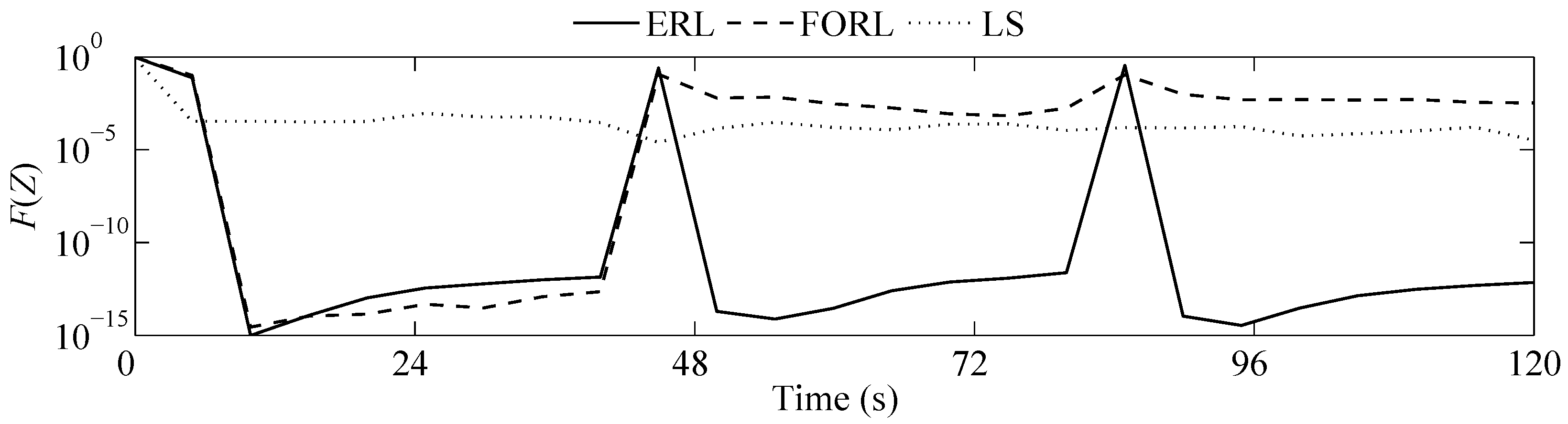
Figure 7 shows the error function values generated by the three algorithms. For the ERL algorithm, $F\left(Z\right)$ varies in the range of (${10}^{-8},{10}^{-4}$), whereas it varies in the range of (${10}^{-2},{10}^{-6}$) for the FORL algorithm. The difference in performance between these two algorithms can be attributed to the improvements to the ERL algorithm mentioned in Section 3.1. First, the agents in the ERL algorithm are able to mutually cooperate and coordinate towards a common goal by virtue of their adaptive learning rates. By contrast, the agents in the FORL algorithm lack the ability to coordinate with each other due to their fixed learning rate. Second, the agents in the ERL algorithm accumulate separate value functions corresponding to the three different load rate intervals. Therefore, they have access to various solutions that are effective under different load rates. In the case of the FORL algorithm, only one table of value functions is used to store the search experience gained when operating in all load rate intervals. As mentioned in Section 3, the optimal parameters are influenced by the load rate. It is clear in Figure 6 that the load rates on the sixth and seventh days are quite different from those on the first five days. The initial values set in the LS algorithm may be close to the optima of the model parameters corresponding to the last two days, but far from the optima for the first five days. Consequently, the LS algorithm falls into local optima during the first five days and cannot find effective solutions to the model until the beginning of the sixth day. We can conclude from this observation that the LS algorithm cannot avoid being influenced by the chosen initial values despite the relevant improvements. Thus, the ERL algorithm outperforms the FORL algorithm in terms of modeling accuracy and has an advantage over the LS algorithm in its ability to escape from local optima.

4.1.3. Ward Equivalent Model of a Real Power System

In this case, a real 1209-bus power system operating in China is considered, and a portion of the system with a voltage level below 110 kV is replaced with a Ward equivalent model. A total of 56 buses are to be reduced, and the Ward equivalent model involves 6 boundary buses and 66 parameters to be identified. Under the same sampling rate and the same set of algorithms as in the previous case, the ERL, FORL and LS algorithms are each employed to identify the parameters of the model. Suppose that each bus load in the 1209-bus power system varies proportionally to the load rate profile shown in Figure 6.

Figure 8 shows the error function values generated by the three algorithms for the real power system. For the ERL algorithm, $F\left(Z\right)$ varies in the range of (${10}^{-6},{10}^{-2}$), whereas it varies in the ranges of (${10}^{-4},{10}^{-2}$) and (${10}^0,{10}^2$) for the FORL and LS algorithms, respectively. Compared with the results for the IEEE 57-bus power system, the models optimized by the three algorithms in this case are less accurate because the reduced network contains more buses and branches and the model involves more parameters to be identified. Consistent with the conclusions drawn in the previous case, the results obtained on the real power system also indicate that the ERL algorithm outperforms the FORL and LS algorithms in terms of accuracy and the ability to avoid local optima.

4.2. Accuracy in Non-Base Scenarios

In this analysis, the Ward equivalent model is connected to the power supply network in place of the original area load. By comparing the power flow results for the original and equivalent systems, the accuracy of the Ward equivalent model is tested in the following non-base scenarios.

• Scenario 1: the voltage magnitude of Generator 2 (G2), $V_{\mathrm{G}2}$, varies with a deviation $\Delta V_{\mathrm{G}2}$ ranging from $-10\%$ to $+10\%$ of its nominal value.
• Scenario 2: the active power output of G12, $P_{\mathrm{G}12}$, varies with a deviation $\Delta P_{\mathrm{G}12}$ ranging from $-10\%$ to $+10\%$ of its nominal value.
• Scenario 3: the apparent power of the total load in the power supply network, $S_{\mathrm{Load}}$, varies with a deviation $\Delta S_{\mathrm{Load}}$ ranging from $-10\%$ to $+10\%$ of its nominal value.

Moreover, the following two metrics are employed to evaluate the accuracy of the model under system disturbances: the relative magnitude of the error between the complex power injected into the original area load and the area load model ($E_{\mathrm{S}}$) and the relative magnitude of the error between the voltages at the boundary buses in the original and equivalent systems ($E_{\mathrm{V}}$). These two metrics are formulated below:

$$\left\{\begin{array}{cccc}\hfill E_{\mathrm{S}}& =\hfill & \underset{i}{max}& \left(|\stackrel{·}{V_i}\stackrel{*}{I_i}-\stackrel{·}{V_i^{\mathrm{e}}}\stackrel{*}{I_i^{\mathrm{e}}}|/|\stackrel{·}{V_i}\stackrel{*}{I_i}|\right)(i=1,2,\cdots ,n)\\ \hfill E_{\mathrm{V}}& =\hfill & \underset{i}{max}& \left(|\stackrel{·}{V_i}-\stackrel{·}{V_i^{\mathrm{e}}}|/|\stackrel{·}{V_i}|\right)(i=1,2,\cdots ,n)\end{array}\right.$$

(7)

where $\stackrel{·}{V_i}$ and $\stackrel{*}{I_i}$ are the voltage phasor and the conjugate of the current phasor, respectively, measured at the i-th boundary bus in the original power system; voltage and current phasors with a superscript of ‘$\mathrm{e}$’ denote the corresponding quantities calculated for the equivalent system; and n is the number of boundary buses.

4.2.1. Accuracy Verification for the ERL Algorithm

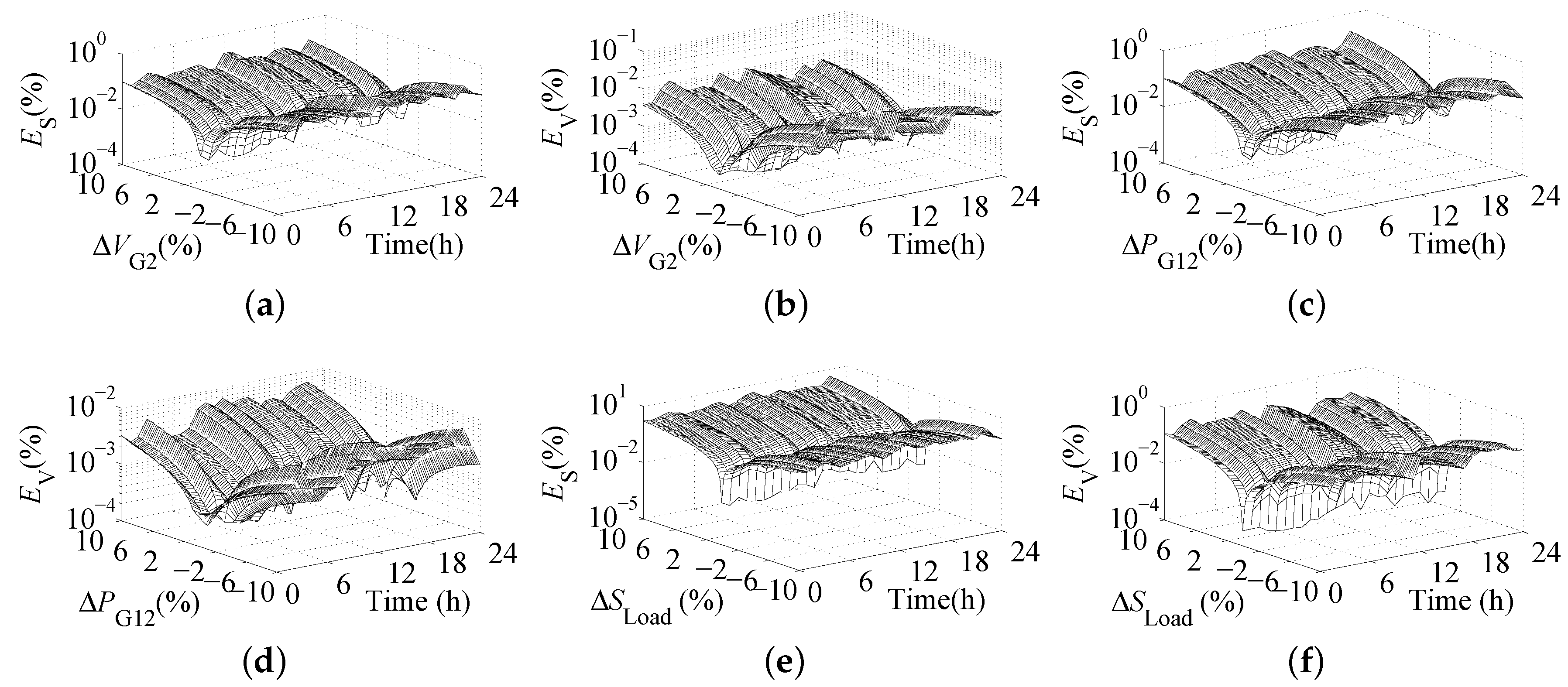
Figure 9 shows the test results obtained using the ERL algorithm in all scenarios during the seventh day on the IEEE 57-bus power system. In all plots, the errors increase when $V_{\mathrm{G}2}$, $P_{\mathrm{G}12}$ and $S_{\mathrm{Load}}$ deviate from their nominal values. In Scenarios 1 and 2, as seen from Figure 9a to Figure 9d, all relative errors are below $0.1\%$, and $E_{\mathrm{V}}$ is no more than $0.01\%$. These results indicate that the model remains accurate when the voltage magnitude or active power output of a generator varies around its nominal value. In Scenario 3, the load changes result in large variations of the power flow distribution, so the values of $E_{\mathrm{S}}$ and $E_{\mathrm{V}}$ are both larger than in the other scenarios. Nevertheless, the largest error in Figure 9e is only approximately $1\%$. Therefore, the test results presented in Figure 9 demonstrate that the proposed Ward equivalent model is able to accurately represent the area load in the above scenarios and that the ERL algorithm can also accurately track the parameters in an online manner.

4.2.2. Accuracy Comparison with Other Algorithms

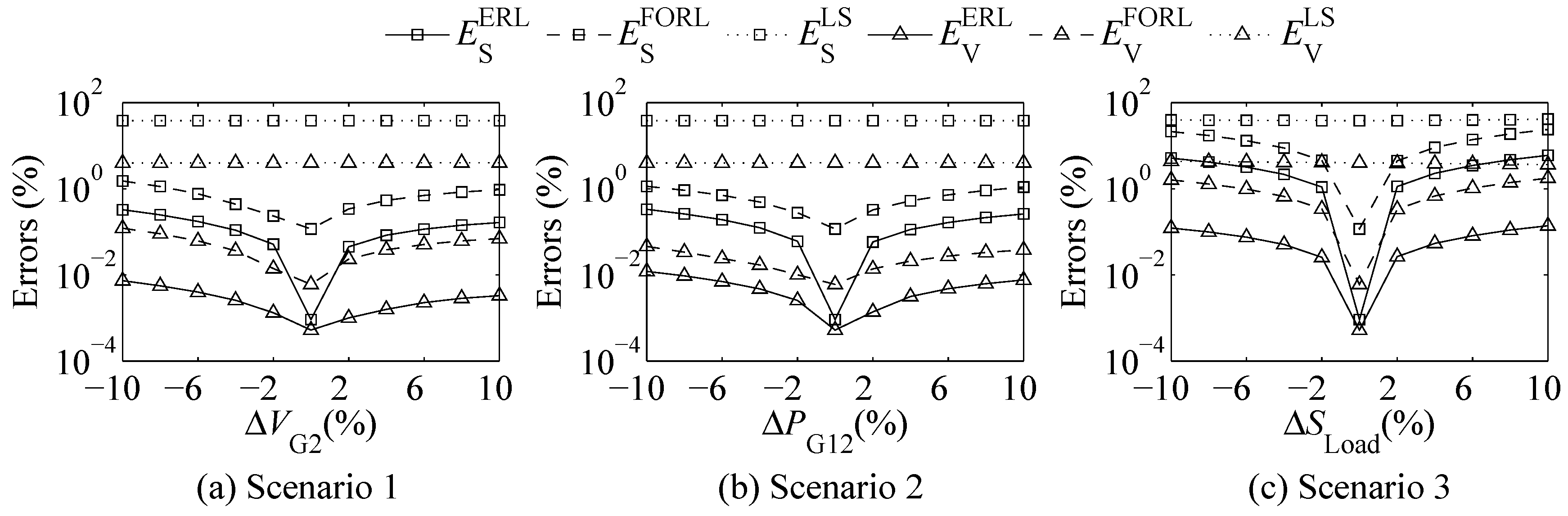
The tracking results obtained using the ERL, FORL and LS algorithms for the Ward equivalent model at 02:23 on the fifth day in the three scenarios above are shown in Figure 10. The two types of errors are distinguished by different marker shapes, and the algorithms are distinguished by different line types. In this study, $\Delta V_{\mathrm{G}2}$, $\Delta P_{\mathrm{G}12}$ and $\Delta S_{\mathrm{Load}}$ vary from $-10\%$ to $+10\%$ of the corresponding nominal values. In Figure 10a,b, the $E_{\mathrm{S}}$ and $E_{\mathrm{V}}$ values obtained using the ERL algorithm are much lower than those obtained using the FORL and LS algorithms. More specifically, in scenarios 1 and 2, the ERL algorithm achieves values of $E_{\mathrm{S}}$ that are below $1\%$ and values of $E_{\mathrm{V}}$ that are below $0.01\%$. In Scenario 3, when all loads in the power supply network vary by $10\%$, the $E_{\mathrm{S}}$ values obtained by the ERL algorithm are no greater than $10\%$. In all three scenarios, the models trained by both the ERL and FORL algorithms are more accurate when the total load deviation is within $-2\%$ to $2\%$ of the nominal value. By contrast, for the LS algorithm, $E_{\mathrm{S}}$ remains in the range of ($10\%,100\%$) in all three scenarios, indicating that this algorithm always fails to find effective parameters for the model at this time instant. Therefore, the area load model optimized using the ERL algorithm is more accurate than those optimized using the other two algorithms in all three scenarios.

To further examine the stability of the algorithms, two statistically significant metrics are employed to assess the average errors when the optimized models are subjected to perturbations:

$$\left\{\begin{array}{ccc}\hfill {\overline{E}}_{\mathrm{S}}& =\hfill & 1/n_{\Delta }\sum _{k=1}^{n_{\Delta }}{E}_{\mathrm{S},k}\\ \hfill {\overline{E}}_{\mathrm{V}}& =\hfill & 1/n_{\Delta }\sum _{k=1}^{n_{\Delta }}{E}_{\mathrm{V},k}\end{array}\right.$$

(8)

where $n_{\Delta }$ is the number of samples of system perturbations $\Delta V_{\mathrm{G}2}$, $\Delta P_{\mathrm{G}12}$ and $\Delta S_{\mathrm{Load}}$. Intuitively, calculating ${\overline{E}}_{\mathrm{S}}$ means compressing the 3-D plot shown in Figure 9a along the $\Delta V_{G2}$ axis; then, at each time instant, ${\overline{E}}_{\mathrm{S}}$ is the average of the values of $E_{\mathrm{S}}$ obtained as $\Delta V_{G2}$ varies. ${\overline{E}}_{\mathrm{V}}$ can similarly be calculated by averaging the values of $E_{\mathrm{V}}$. We present the results for ${\overline{E}}_{\mathrm{S}}$ and ${\overline{E}}_{\mathrm{V}}$ throughout the 5th day in Figure 11 and Figure 12, respectively. According to these figures, the ERL algorithm is much more accurate than the FORL and LS algorithms under all three scenarios on this day. Moreover, the average errors of the FORL algorithm can be quite large at several specific time instants, which indicates that the stability of the FORL algorithm is not satisfactory.

4.2.3. Accuracy Comparison with Another Model

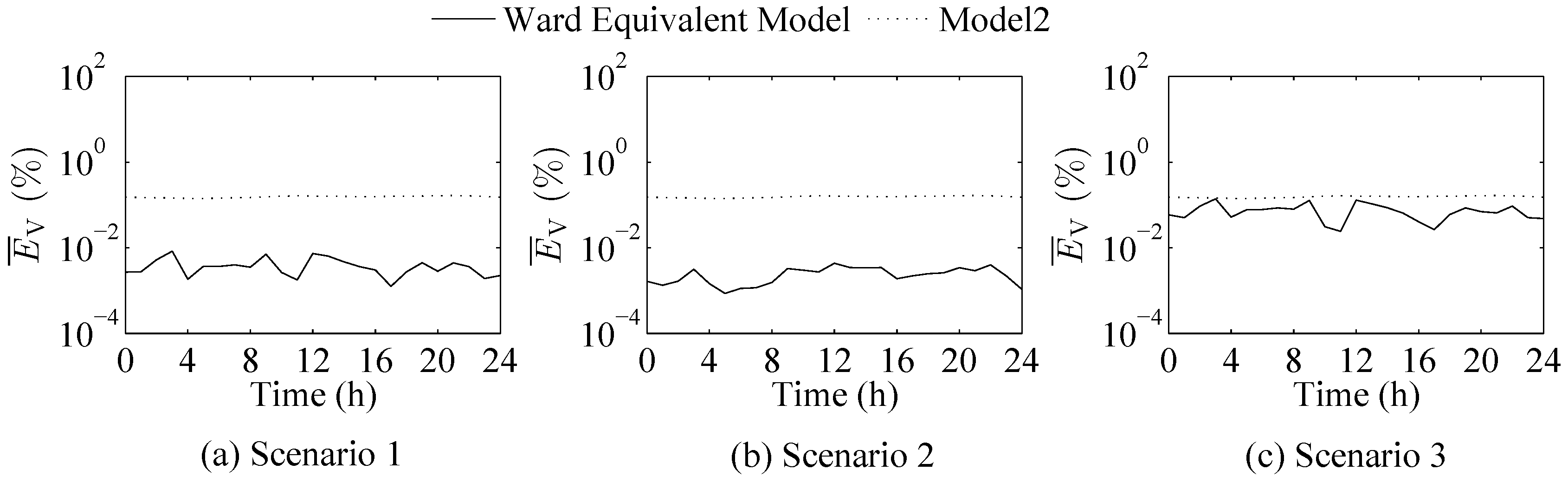
As a basis for comparison in this analysis, we consider the model for the area load in the 57-bus power system that is presented in [35]; this model is composed of a fictitious load bus and fictitious branches. The parameters of the model from [35] are tracked in an online manner by the ERL algorithm under the same load profile. Figure 13 presents the test results at the same time instant considered in Section 4.2.2. In this figure, the superscript ‘Ward’ represents the Ward equivalent model, and the superscript ‘Model2’ represents the model presented in [35]. The two types of errors are distinguished by different marker shapes. Figure 13a,b show that in Scenarios 1 and 2, the $E_{\mathrm{S}}$ and $E_{\mathrm{V}}$ values for the Ward equivalent model are much lower than those for the model from [35] when $\Delta V_{\mathrm{G}2}$ and $\Delta P_{\mathrm{G}12}$, respectively, vary from $-10\%$ to $10\%$ of the corresponding nominal value. In Scenario 3, the two models exhibit similar performance, but the $E_{\mathrm{S}}$ and $E_{\mathrm{V}}$ values for the Ward equivalent model are much lower than those for the model from [35] when $\Delta S_{\mathrm{Load}}$ is within $-2\%$ to $2\%$ of the nominal $S_{\mathrm{Load}}$ value. According to these results, the Ward-equivalence-based area load model proposed in this paper is more accurate than the model previously proposed in [35].

As in the previous comparison, the average errors ${\overline{E}}_{\mathrm{S}}$ and ${\overline{E}}_{\mathrm{V}}$ of the two models during the 5th day are presented in Figure 14 and Figure 15, respectively. We can conclude from these figures that the accuracy of both models is stable under system perturbations. However, the Ward equivalent model is much more accurate than the model previously proposed in [35] on this day.

5. Conclusions

This paper proposes an area load modelling approach for simplifying the topological structure of power networks and introduces an ERL algorithm for the online tracking of the model parameters. Unlike the models utilized in previous works, the proposed Ward equivalent area load model involves multiple boundary buses and explicitly considers the static load characteristics of the voltage. According to the results obtained for three simulation cases, the proposed ERL algorithm is capable of tracking both step-changing and time-varying parameters in an online manner and can improve the accuracy of the proposed Ward equivalent model compared with the FORL and LS algorithms. Therefore, the online modelling approach presented in this work can serve as a foundation for the real-time dispatch and control of power systems.

References

- Wen, J.Y.; Wu, Q.H.; Nuttall, K.I.; Shimmin, D.W.; Cheng, S.J. Construction of power system load models and network equivalence using an evolutionary computation technique. Int. J. Electr. Power Energy Syst. 2003, 25, 293–299. [Google Scholar] [CrossRef]
- Arif, A.; Wang, Z.; Wang, J.; Mather, B.; Bashualdo, H.; Zhao, D. Load Modeling: A Review. IEEE Trans. Smart Grid 2017. [Google Scholar] [CrossRef]
- Zhao, J.; Wang, Z.; Wang, J. Robust Time-Varying Load Modeling for Conservation Voltage Reduction Assessment. IEEE Trans. Smart Grid 2016. [Google Scholar] [CrossRef]
- Fahmy, O.; Attia, A.; Badr, M. A novel analytical model for electrical loads comprising static and dynamic components. Electr. Power Syst. Res. 2007, 77, 1249–1256. [Google Scholar] [CrossRef]
- Casolino, G.; Losi, A. Load Area model accuracy in distribution systems. Electr. Power Syst. Res. 2017, 143, 321–328. [Google Scholar] [CrossRef]
- Tulabing, R.; Yin, R.; DeForest, N.; Li, Y.; Wang, K.; Yong, T.; Stadler, M. Modeling study on flexible load’s demand response potentials for providing ancillary services at the substation level. Electr. Power Syst. Res. 2016, 140, 240–252. [Google Scholar] [CrossRef]
- Ward, J.B. Equivalent circuits for power-flow studies. Electr. Eng. 1949, 68, 794. [Google Scholar] [CrossRef]
- Ângelos, E.W.S.; Asada, E.N. Improving State Estimation With Real-Time External Equivalents. IEEE Trans. Power Syst. 2016, 31, 1289–1296. [Google Scholar] [CrossRef]
- Van Amerongen, R.A.M.; van Meeteren, H.P. A Generalised Ward Equivalent for Security Analysis. IEEE Trans. Power Appar. Syst. 1982, PAS-101, 1519–1526. [Google Scholar] [CrossRef]
- Neto, A.C.; Rodrigues, A.B.; Prada, R.B.; da Silva, M.D. External Equivalent for Electric Power Distribution Networks With Radial Topology. IEEE Trans. Power Syst. 2008, 23, 889–895. [Google Scholar] [CrossRef]
- Hu, F.; Sun, K.; Rosso, A.D.; Farantatos, E.; Bhatt, N. Measurement-Based Real-Time Voltage Stability Monitoring for Load Areas. IEEE Trans. Power Syst. 2016, 31, 2787–2798. [Google Scholar] [CrossRef]
- Wei, J.L.; Wang, J.H.; Wu, Q.H.; Lu, N. Power system aggregate load area modelling by particle swarm optimization. Int. J. Autom. Comput. 2005, 2, 171–178. [Google Scholar] [CrossRef]
- Regulski, P.; Vilchis-Rodriguez, D.S.; Djurovi, S.; Terzija, V. Estimation of Composite Load Model Parameters Using an Improved Particle Swarm Optimization Method. IEEE Trans. Power Deliv. 2015, 30, 553–560. [Google Scholar] [CrossRef]
- Wang, Z.; Wang, J. Time-Varying Stochastic Assessment of Conservation Voltage Reduction Based on Load Modeling. IEEE Trans. Power Syst. 2014, 29, 2321–2328. [Google Scholar] [CrossRef]
- Zhang, Q.; Lai, K.K.; Niu, D.; Wang, Q.; Zhang, X. A Fuzzy Group Forecasting Model Based on Least Squares Support Vector Machine (LS-SVM) for Short-Term Wind Power. Energies 2012, 5, 3329–3346. [Google Scholar] [CrossRef]
- Guo, X.; Kang, L.; Yao, Y.; Huang, Z.; Li, W. Joint Estimation of the Electric Vehicle Power Battery State of Charge Based on the Least Squares Method and the Kalman Filter Algorithm. Energies 2016, 9, 100. [Google Scholar] [CrossRef]
- Kim, T.; Ivantysynova, M. Active Vibration Control of Swash Plate-Type Axial Piston Machines with Two-Weight Notch Least Mean Square/Filtered-x Least Mean Square (LMS/FxLMS) Filters. Energies 2017, 10, 645. [Google Scholar] [CrossRef]
- Weron, R. Electricity price forecasting: A review of the state-of-the-art with a look into the future. Int. J. Forecast. 2014, 30, 1030–1081. [Google Scholar] [CrossRef]
- Cincotti, S.; Gallo, G.; Ponta, L.; Raberto, M. Modeling and forecasting of electricity spot-prices: Computational intelligence vs classical econometrics. AI Commun. 2014, 27, 301–314. [Google Scholar]
- Amjady, N.; Keynia, F. Day ahead price forecasting of electricity markets by a mixed data model and hybrid forecast method. Int. J. Electr. Power Energy Syst. 2008, 30, 533–546. [Google Scholar] [CrossRef]
- Han, C.; Yang, B.; Bao, T.; Yu, T.; Zhang, X. Bacteria Foraging Reinforcement Learning for Risk-Based Economic Dispatch via Knowledge Transfer. Energies 2017, 10. [Google Scholar] [CrossRef]
- Zhao, H.; Wang, Y.; Guo, S.; Zhao, M.; Zhang, C. Application of a Gradient Descent Continuous Actor-Critic Algorithm for Double-Side Day-Ahead Electricity Market Modeling. Energies 2016, 9, 725. [Google Scholar] [CrossRef]
- Xu, Y.L.; Zhang, W.; Liu, W.X.; Ferrese, F. Multiagent-Based Reinforcement Learning for Optimal Reactive Power Dispatch. IEEE Trans. Syst. Man Cybern. Part C Appl. Rev. 2012, 42, 1742–1751. [Google Scholar] [CrossRef]
- Sutton, R.S.; Barto, A.G. Reinforcement Learning: An Introduction. IEEE Trans. Neural Netw. 1998, 9, 1054. [Google Scholar]
- Thorndike, E.L. Animal Intelligence. Psych Revmonog 1911, 8, 207–208. [Google Scholar]
- Machinery, C. Computing machinery and intelligence-AM Turing. Mind 1950, 59, 433. [Google Scholar]
- Wu, Q.H.; Liao, H.L. High-dimensional Function Optimisation by Reinforcement Learning. In Proceedings of the 2010 IEEE Congress on Evolutionary Computation (CEC), Barcelona, Spain, 18–23 July 2010; pp. 1–8. [Google Scholar]
- Hansen, N.; Müller, S.D.; Koumoutsakos, P. Reducing the Time Complexity of the Derandomized Evolution Strategy with Covariance Matrix Adaptation (CMA-ES). Evol. Comput. 2003, 11, 1–18. [Google Scholar] [CrossRef] [PubMed]
- Matignon, L.; Laurent, G.J.; Fort-Piat, N.L. Hysteretic q-learning: An algorithm for decentralized reinforcement learning in cooperative multi-agent teams. In Proceedings of the 2007 IEEE/RSJ International Conference on Intelligent Robots and Systems, San Diego, CA, USA, 29 October–2 November 2007; pp. 64–69. [Google Scholar]
- Kundur, P. Power System Stability and Control; McGraw-Hill: New York, NY, USA, 1994. [Google Scholar]
- He, R.M.; Ma, J.; Hill, D.J. Composite load modeling via measurement approach. IEEE Trans. Power Syst. 2006, 21, 663–672. [Google Scholar]
- Ma, J.; Han, D.; He, R.M.; Zhao, Y.D.; Hill, D.J. Reducing Identified Parameters of Measurement-Based Composite Load Model. IEEE Trans. Power Syst. 2008, 23, 76–83. [Google Scholar] [CrossRef]
- Ma, J.; Han, D.; He, R.M. Measurement-based load modeling: Theory and application. Sci. China Ser. E Technol. Sci. 2007, 50, 606–617. [Google Scholar]
- Claus, C.; Boutilier, C. The dynamics of reinforcement learning in cooperative multiagent systems. In Proceedings of the Fifteenth National/Tenth Conference on Artificial Intelligence/Innovative Applications of Artificial Intelligence, Madison, WI, USA, 27–29 July 1998; pp. 746–752. [Google Scholar]
- Wen, J.Y.; Jiang, L.; Wu, Q.H.; Cheng, S.J. Power system load modeling by learning based on system measurements. IEEE Trans. Power Deliv. 2003, 18, 364–371. [Google Scholar] [CrossRef]
- Subcommittee, P.M. IEEE Reliability Test System. IEEE Trans. Power Appar. Syst. 1979. [Google Scholar] [CrossRef]
Figure 1.
Area load modeling in the IEEE 57-bus power system. (a) The 57-bus power system with an area load; (b) the Ward equivalent model of the area load.
Figure 2.
Flowchart of the online parameter tracking process implemented by means of the enhanced reinforcement learning (ERL) algorithm.
Figure 3.
Mapping from intervals to parallel tables.
Figure 4.
Coefficients for the single ZIP load. (a) Coefficients of active power; (b) coefficients of reactive power.
Figure 5.
Objective function values obtained by the three algorithms.
Figure 6.
Weekly load profile of the area load in the 57-bus power system.
Figure 7.
Error function values over seven days on the IEEE 57-bus power system.
Figure 8.
Error function values over seven days on the 1209-bus power system.
Figure 9.
Relative errors of the Ward equivalent model as obtained using the ERL algorithm in the different scenarios. (a) in Scenario 1; (b) in Scenario 1; (c) in Scenario 2; (d) in Scenario 2; (e) in Scenario 3; (f) in Scenario 3.
Figure 10.
Relative errors produced by the three algorithms in the different scenarios.
Figure 11.
Mean complex power errors produced by the three algorithms in the different scenarios.
Figure 12.
Mean voltage errors produced by the three algorithms in the different scenarios.
Figure 13.
Relative errors produced by the two models in the different scenarios.
Figure 14.
Mean complex power errors produced by the two models in the different scenarios.
Figure 15.
Mean voltage errors produced by the two models in the different scenarios.