Research on Exergy Flow Composition and Exergy Loss Mechanisms for Waxy Crude Oil Pipeline Transport Processes


Key Lab of Ministry of Education for Enhancing the Oil and Gas Recovery Ratio, Northeast Petroleum University, Daqing, 163318, China
*
Author to whom correspondence should be addressed.
Energies 2017, 10(12), 1956; https://doi.org/10.3390/en10121956
Submission received: 19 October 2017
/
Revised: 19 November 2017
/
Accepted: 21 November 2017
/
Published: 24 November 2017
Abstract
:The basic theory of exergy was used to derive the formulae of physical and chemical exergy in the process of pipeline transportation, combined with the effect of wax deposition on the thermodynamic parameters including specific heat, density, chemical potential and concentration gradient. On the basis of this, the expression of various exergy losses were derived, and the exergy balance model was then built in the process. For the case study, a waxy crude oil pipeline in China was selected. The mechanism for how wax deposition affected the physical and chemical exergy loss was studied through analyzing the axial pipeline distribution of pressure, temperature, flow rate and thickness of insulation layer. Finally, under the design flow of 66 × 103 kg·h−1, the orthogonal experimental analysis method was used for comparing the degree of specific factors which could influence the total exergy efficiency. The highest exergy efficiency combination of working conditions was then determined. This research could provide a theoretical basis for guiding safe and economic operation in the actual pipeline transportation process.
1. Introduction
Most Chinese crude oil is high-pour-point and viscous, waxy crude oil; it generally needs to be heated for transportation [1,2]. In the process of transportation, the oil pump assembly should be set to overcome the head loss. Meanwhile, in order to effectively prevent the tube from condensation, it is also necessary to set the heating devices to maintain the minimum oil temperature above the condensation point. This transportation equipment consumes a lot of energy, especially for those pipelines with long distance and low throughput, for which the heating fuel consumption could account for 0.25 to 0.35% of the transportation volume [3]. With the increasing demand for crude oil, the consumption of pipelines will be further increased, which means that the economic operation of pipelines faces greater challenges. Therefore, it is of great significance to carry out an energy-consumption analysis of waxy crude oil pipelines.
Calculating energy efficiency is the traditional method of energy-consumption analysis, in this method, only the “quantity” attribute of energy is considered. However, energy also has another attribute of “quality,” called exergy, which refers to the maximum working capacity [4]. Energy with a large “quantity” but low “quality” in a system would have a low working ability. If we took the traditional way to analyze such a system, the “quantity” of energy would be treated as the key point to improve energy utilization, the investment in equipment would be large, and the economy of this system would be poor. Compared with the traditional analysis method, and exergy analysis can reveal the essence for the reduction of energy quality and energy levels, and comprehensively identify the weaknesses in an energy system, so that reasonable energy saving measures can be put forward, which make energy utilization more efficient and economical.
According to the capacity of doing work in different potential fields, exergy can be divided into two categories: physical exergy and chemical exergy. In 1965, Persian Yake Vic advocated the concept of constrained and non-constrained balance, which laid the foundation for distinguishing the difference between the physical exergy and chemical exergy of a material system [5]. In 1984, Nabusawatorao proposed selecting the general formulae according to the types of fuels, and provided general formulae for liquid and solid fuels [6]. Afterwards, in 1988, Zhu introduced the deriving process of chemical diffusion exergy in the general thermodynamic system in his book “The Analysis of Energy System by Exergy” for the first time [7]. With the continuous improvement of the theory of exergy, some experts and scholars applied exergy to energy-consumption analyses of the pipeline transportation process, and made certain achievements. In 2009, M.Chaczykowski et al. analyzed the gas system of Yamal-Europe based on the exergy theory, in which the effective energy and the energy loss in the process of gas transmission were determined, then the position where the exergy loss occurred and the magnitude of the energy loss was also given [8]. In 2013, M.Ameri and M.Askari et al. carried out exergy and economic analyses on a crude oil transportation pipeline and related pump stations in Iran, in which the exergy loss and exergy efficiencies were calculated for each part of the whole system and itself [9]. In addition, to reduce the flow resistance, the method to heat crude oil with waste gas was proposed. In 2015, Cheng et al. took a crude oil pipeline as an example, and discussed the distribution of exergy flow and the rules for how thermal and pressure exergy transferred and was delivered, providing the theoretical and rational basis for the energy-saving calculation of a pipeline system [10].
It is noteworthy that many experts and scholars have done a great deal of research into exergy analyses of general pipeline transportation processes, however, for the pipeline transportation process of waxy crude oil, their studies might be more reasonable and accurate if they had considered wax precipitation, which can impact the physical and chemical exergy. In fact, wax precipitation will lead to a change in some corresponding thermodynamic parameters, and the thermal exergy, pressure exergy, chemical reaction exergy and chemical diffusion exergy will be thus be affected [11]. According to the characteristics of waxy crude oil, this paper deduced the calculation method for physical exergy and chemical exergy in the process of waxy crude oil pipeline transportation. Furthermore, a waxy crude oil transportation pipeline from an oilfield in eastern China was taken as an example, an exergy analysis of the transportation system was carried out, the distribution of various types of exergy loss was provided, and the reasons for this phenomenon were analyzed.
2. Physical and Chemical Exergy in the Process of a Waxy Crude Oil Pipeline Transport Process
The potential fields can be divided into physical fields and potential chemical fields [12]. According to the working ability for different potential fields, we can divide the exergy into two categories, physical exergy and chemical exergy, in the process of waxy crude oil pipeline transportation [13].
2.1. The Physical Exergy of Waxy Crude Oil Pipeline Transportation
The research done in this paper was based on a horizontal pipe, and the waxy crude oil has no change of elevation in the process of pipeline transportation, so the potential exergy can be ignored [14]. Owing to the fact that the process of pipeline transportation can be treated as steady-flow, and the speed exergy is smaller compared to the enthalpy, this can also be ignored. To sum up, the physical exergy can be divided into two parts: thermal exergy and pressure exergy.
Thus, the physical exergy can be expressed as:
where and respectively represent the thermal exergy and the pressure exergy of stable material flow.
2.1.1. The Calculation of Thermal Exergy
The exergy caused by the temperature difference is referred as thermal exergy:
If the range of the temperature is not large, taking the average as 2.133 kJ·kg−1·K−1 under the temperature of T0~T, and the non-dimensional temperature is introduced, the formula will be simplified as:
With the increase of the transportation distance, the crude oil temperature drops to the wax precipitation point, then the original dissolved waxy molecules will separate out due to their different molecular weight. Therefore, the specific heat capacity of waxy crude oil changes with temperature, which should not be ignored for precise calculations. According to the capacity–temperature curve, based on the wax precipitation point TSL and the maximum specific heat capacity temperature Tcmax, the specific heat capacity which changes with the temperature can be divided into three regions:
When T > TSL:
where is the specific heat capacity, and is the relative density of oil at 15 °C.
When TSL > T > Tcmax, with the drop of oil temperature, the wax precipitation rate of the unit temperature drop gradually increases. This process released more latent crystallization heat, so the specific heat increases gradually. The relationship between specific heat capacity and temperature can be fitted by the following formula:
where A and n are relatively the constants varying with the crude oil.
When T < Tcmax, most of the wax in the crude oil has been precipitated with the decrease in temperature. As the cooling process continues, the specific heat capacity of crude oil will decrease, and the relationship between it and the temperature can be fitted by the following formula:
where B and m are relatively the constants varying with the crude oil.
In this paper, the conditions under which the specific heat capacity changes with the temperature can be summarized as:
- When the temperature is lower than 22 °C:
- When the temperature is between 22~48 °C:
- When the temperature is greater than 48 °C:
where c is the specific heat capacity of crude oil, and T is the temperature of crude oil.
2.1.2. The Calculation of Pressure Exergy
The exergy which is caused by the pressure difference is referred as pressure exergy:
The relationship between the density and temperature of crude oil is:
where ρ is the density of crude oil, ρ20 is the density of crude oil at 20 °C, and ξ is temperature coefficient.
Then the pressure exergy at any temperature can be expressed as:
For the crude oil in the process of transportation, the above formulae indicate:
- In the certain environmental state of (T0, P0), the thermal exergy ext and pressure exergy exp are all state parameters of the materials, moreover, thermal exergy ext is only a function of temperature and pressure exergy exp is a function of both pressure and temperature;
- The crude oil properties have no effect on pressure exergy exp. Although thermal exergy ext relates to the crude oil properties, it only depends on the constant pressure-specific heat cp. Therefore, this simple relation will bring about convenience for calculating and analyzing the physical exergy of crude oil.
2.2. The Chemical Exergy of Waxy Crude Oil Pipeline Transportation
The chemical exergy of materials refers to the maximum working ability, which is caused by chemical non-equilibrium between materials and their environment. The chemical exergy of a thermodynamic system can be considered as the sum of chemical reaction exergy and chemical diffusion exergy:
2.2.1. The Chemical Reaction Exergy of Waxy Crude Oil Transportation
In principle, the chemical reaction exergy of fuels has little difference to other compounds. As long as its composition and enthalpy are given, it can be calculated according to the corresponding equations [15]. However, the fuels in practical use usually contain many complex substances, of which the compositions are difficult to accurately determine, especially for those solid fuels which are usually composed of unstable molecular aggregations. Thus, for general liquid and solid fuels, including coal and oil, various semi-empirical formulae and approximate formulae of fuel exergy are often adopted in engineering exergy analysis. The frequently-used approximate algorithms now include the “Rant method”, “Nabusawatorao method” and “Szargut-Styrylska method” [16].
In the literature [17], various approximate algorithms were used to calculate the chemical reaction exergy of the crude oil in Shengli, Daqing and the other five oil fields in China. All the deviations were based on the “Szargut-Styrylska method”, which showed that all the deviations were less than 2.3%, close to the previous results for kerosene’s chemical reaction exergy. This indicates that this estimation method for the chemical reaction exergy of crude oil was available, the numerical value of the chemical reaction exergy was in the range of the gross heat value and the low heat value, and that the reaction exergy of crude oil increased with the H-C ratio (Hydrogen-Carbon ratio).
In the process of pipeline transportation, the chemical reaction exergy of crude oil is not completely invariant. This is because the dissolved wax gradually separates out and deposits on the pipeline wall, leading to a composition change of chemical elements, and the loss of chemical reaction exergy. However, in the process of pipeline transportation, the loss of elements in this part is smaller than that of the crude oil itself, and it can be ignored in the actual engineering calculation accordingly [18].
2.2.2. The Chemical Diffusion Exergy of Waxy Crude Oil Transportation
In the process of waxy crude oil pipeline transportation, with the increase of wax precipitation, the molecular concentration gradient severely changes [19], so diffusion exergy cannot be ignored [20]. In this paper, 1 atm and 298.15 K are used as the reference pressure and temperature of the environment, and the crude oil in the pipeline transportation process is regarded as the multi-component system, with temperature T, pressure P, and a constrained equilibrium state. The standard substances of the environment are components of alkanes, cycloalkanes etc., the mole of which is the same as that of crude oil at 298.15 K and 1 atm.
When the multi-component system undergoes a reversible process and achieves a non-constrained equilibrium state, there will exist mass exchange between the system and the environment, meanwhile, the maximum useful work is made to the external world. If the system and the environment formed an adiabatic joint system C, there would be a work exchange with the external world in this process, and the exchange work is the maximum useful work Wmax. According to the first law of thermodynamics , there is:
In the state of non-constrained equilibrium, the mole number of components in the multi-component system is the same as that of any state, therefore, the expression of diffusion exergy of 1 kmol in the multi-component system can be further expressed as a more general form:
Since the system compositions are complex in pipeline transportation, this cannot be treated as the ideal solution. The calculation of the chemical diffusion exergy can be referred to the method of the non-ideal solution, and the corresponding molar diffusion exergy can be transformed into:
where and are respectively the activity coefficients of component i in a state of constrained and non-constrained equilibrium; and and are respectively the molar fractions of component i in a state of constrained and non-constrained equilibrium. From this formula, the main two parameters for calculating the chemical diffusion exergy are the activity coefficient r and the molar fraction x.
1. The calculation of the component molar fraction
In this paper, phase equilibrium theory is used to solve the problem of the composition of solid and liquid components in the system. When the thermodynamic system reaches phase equilibrium, the fugacity of each phase state is equal:
The liquid–solid phase fugacity of the component i is:
where and respectively represent the standard-state fugacity of the liquid and solid phase of component i, and and respectively represent the molar volume of the liquid and solid phase of component i.
When the thermodynamic system is in a state of low or medium pressure, there is little influence of the component volume difference on the solid–liquid equilibrium constant, so the effect of the Poynting factor on the equilibrium constant can be neglected; then the liquid–solid equilibrium constant of component i is obtained:
The standard fugacity ratio in Equation (20) can be obtained by the following formula:
where is the dissolved enthalpy of component i.
For isoparaffin and cycloalkanes:
For aromatics:
During the transportation process, when the temperature decreases to the dissolution temperature of component i, the wax molecules which originally dissolved in the crude oil will crystallize and separate out. To calculate the dissolution temperature of the n-alkanes, Won proposed the following Equation [22]:
To determine the dissolution properties of the non-alkane component, Lira-Galeana proposed the following Equation:
To calculate the change of specific heat capacity, the following Equation was taken:
where Mi represents the molar mass of component i.
2. The calculation of the activity coefficient
In this paper, a more accurate theoretical model of the regular solution is adopted to calculate the activity coefficient:
The solubility parameters in this Equation can be represented as , while the can be determined with . According to the Equation (32), the activity coefficient can be obtained by calculating the solubility parameters and molar volume of component i.
The solubility parameters of the liquid phase of n-alkanes can be used with the formula built by Riazi and Al-Sahhaf:
The liquid-phase solubility parameters of other types of hydrocarbons can be used with the formulae built by Leelvanacihkul:
For isoparaffins and cycloalkanes:
For aromatics:
The solid-phase solubility parameters of component i can be calculated by the following Equations:
The solid and liquid molar volume of component i can be calculated by the following Equation:
The formula of the liquid phase density of component i at 25 degrees can be used with the following Equation established by Leelvanaichkul:
For n-alkanes:
For isoparaffins and cycloalkanes:
For aromatics:
3. Exergy Loss and Exergy Efficiency in the Process of Waxy Crude Pipeline Transportation
3.1. The Exergy Balance Equation of the Pipeline Transportation
The total exergy in the process of pipeline transportation is the sum of physical exergy and chemical exergy. The process does not involve chemical reactions, so only the change of pressure exergy, heat exergy and chemical diffusion exergy in the system should be considered. Therefore, the total exergy of pipeline transportation can be written as [23]:
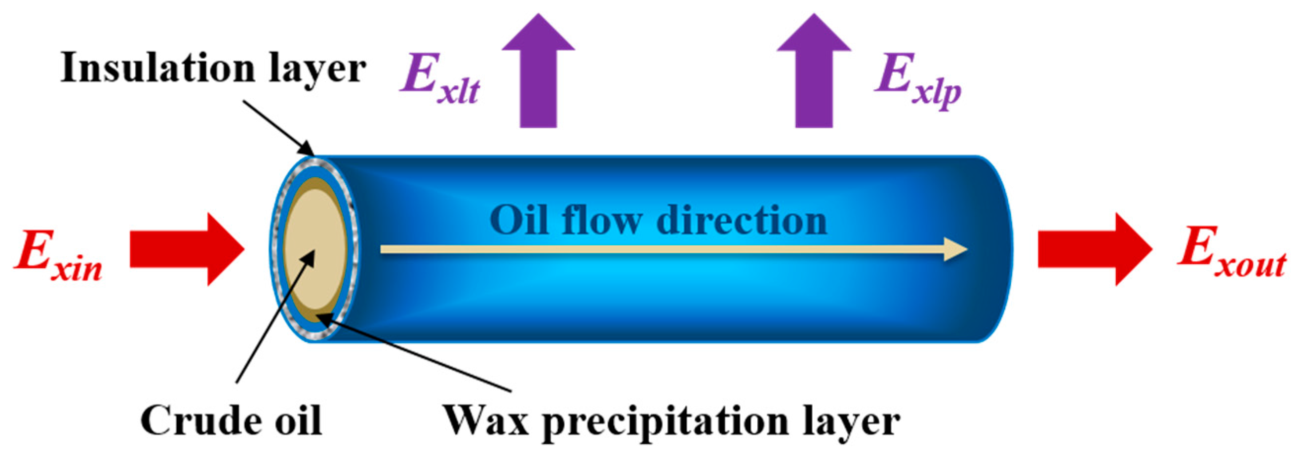
In order to evaluate the energy-saving potential from the aspect of energy quality utilization, a general exergy analysis needs to be carried out for the pipeline transportation system. A model of exergy analysis in the process of pipeline transportation was built as in Figure 1.
According to the exergy analysis model, the exergy balance equation can be written as:
where .
In Equation (41), Exin and Exout are respectively the physical exergy which inflow and outflow from the pipeline; Exlin and Exlout are respectively the internal and external exergy loss of the pipeline.
3.2. The Formula for Calculating the Exergy Loss in Pipeline Transportation
3.2.1. The Exergy Flow Loss in the Pipeline Transportation
1. The loss of thermal exergy
where T1, T2 are the inlet and outlet temperatures of the pipeline respectively, G is mass flow rate of the crude oil, kg·s−1, and is the non-dimensional temperature.
2. The loss of pressure exergy
where P1, P2 are the inlet and outlet pressures of the pipeline, respectively.
3. The loss of chemical diffusion exergy
where M is the molar mass of the crude oil.
3.2.2. The Internal and External Exergy Loss in the Pipeline Transportation
For exothermic objects, when heat and exergy flow out of the objects together, the reduced material flow exergy is:
where the heat loss of the pipeline is:
Thus, the corresponding external heat dissipation exergy loss in the pipeline is:
3.2.3. The Total Exergy Loss in the Process of Pipeline Transportation
According to the sections above regarding the calculation equation of physical and chemical exergy, the material flow exergy can be respectively written as:
where is the exergy flow of the pipeline inlet, and is the exergy flow of the pipeline outlet.
From the two formulae above, the total exergy loss in the process of pipeline transportation can be expressed as:
3.3. The Exergy Efficiency in the Process of Transportation
In the process of energy transmission and conversion, the ratio of the gained exergy Ex,gain to the paid exergy Ex,pay is defined as the exergy efficiency, and is used to express the exergy efficiency [24]:
According to the second law of thermodynamics, any irreversible process will cause exergy loss, therefore the difference between the gained exergy Ex,gain and the paid exergy Ex,pay is the exergy loss:
Additionally, there is:
where is named as the exergy loss coefficient.
4. Application Example Analysis
4.1. Basic Data
For the case study, a typical example of an oil pipeline in an eastern Chinese oil field was taken [17]. The basic operating parameters of the pipeline are shown in Table 1.
Besides, the length of the pipeline is about 18 km, the specification of the diameter is Φ219.1 mm × 5.6 mm.
4.2. Analysis of Exergy Loss in the Process of Pipeline Transportation
The exergy loss for the pipeline system is calculated based on the basic data, and the ratios of various exergy losses to the total exergy loss are shown in Figure 2.
Through analyzing the results in the Figure 2, we can see that the thermal exergy loss occupies a large part, the second level of the ratio is the diffusion exergy loss, and the pressure exergy loss only accounts for about 11%, which illustrates that the process of waxy crude oil transportation is greatly affected by the temperature field, the effect of the wax molecule concentration field is in second place, and the effect of the pressure field is the least strong.
For the total exergy loss, the external thermal exergy loss also accounts for a large part. It can be seen that during actual pipeline transportation, the transmission temperature should be reduced as low as possible under the premise of ensuring the safety of transportation.
The internal exergy loss accounts for a smaller proportion of the total exergy loss compared to the external exergy loss. The sources of the internal exergy loss of the pipeline transportation are mainly three kinds: the pressure differential, the temperature differential and the chemical potential differential. The internal exergy loss is usually caused by the irreversibility of the process, which one can attempt to reduce but not eliminate.
4.3. The Mechanism Analysis of Exergy Loss in the Pipeline Transportation Process
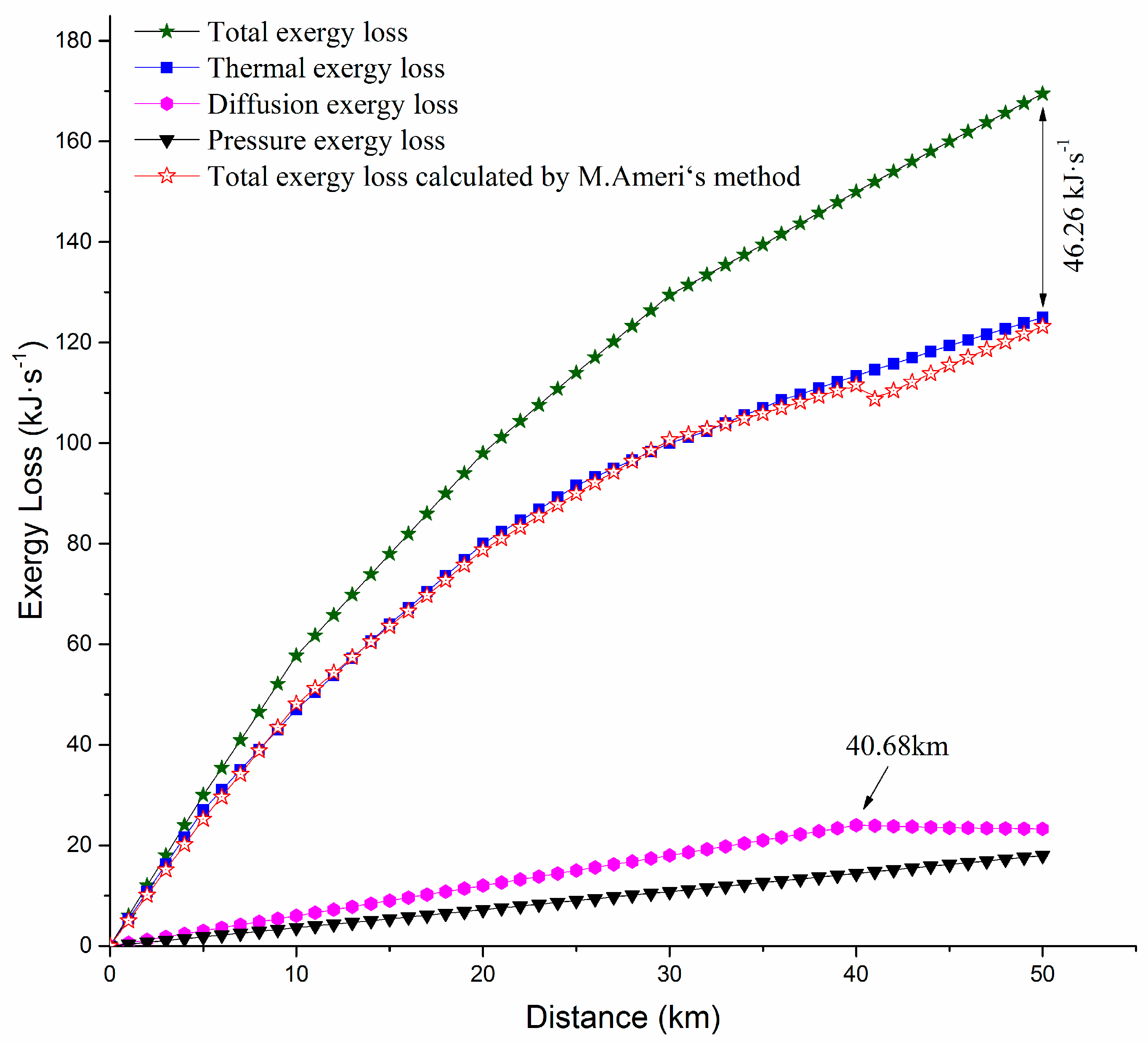
The model mentioned in the above chapters was used to calculate pressure exergy loss, thermal exergy loss, diffusion energy loss and the total exergy loss in the process of pipeline transportation. In 2013, M. Ameri and M. Askari carried out a similar analysis as that in this study, for comparison, their method was used to calculate the total exergy loss for the pipeline selected in this study [9]. The axial distribution curve of various exergy losses is illustrated in Figure 3.
It can be seen from Figure 3 that various exergy losses are increasing along the axial direction of the waxy crude oil pipeline. The thermal exergy loss is far greater than the pressure exergy loss and the diffusion exergy loss. There is little difference between the diffusion exergy loss and the pressure exergy loss.
In the initial stage, the temperature difference between the pipeline and the surrounds is high, which leads to a great decrease in the crude oil temperature, so the thermal exergy loss increases greatly. With the increase in transportation distance, the decreasing tendency of the temperature becomes slow, the reasons can be explained as, on the one hand, due to a part of the wax molecules separating out from the oil flow, releasing the latent heat and slowing down the temperature change; on the other hand, due to the decrease of temperature difference between oil flow and the environment, the heat loss of the pipeline decreases, which also leads to the slowing down of the thermal exergy loss trend.
With the increase of transmission distance, the change of axial diffusion exergy loss is relatively slow. When the transmission temperature is lower than the wax precipitation point, the wax molecules constantly precipitate, and the molecule concentration of the liquid crude oil become small, so the tendency of the diffusion exergy loss increases. After 40.68 km, the precipitation amount of the wax molecules gradually slows down, resulting in a slower trend of diffusion exergy loss.
With the increase in transportation distance, the trend of the pressure exergy loss in the axial pipeline is stable, which can be explained as the pressure exergy being mainly affected by the transportation pressure.
In Figure 3, one can see that between the two curves of total exergy loss, calculated by M. Ameri’s method and the method of this paper, there exists a large deviation, this deviation reaches the maximum value of 46.26 kJ·s−1 at 50 km. The reason for this is the neglect of wax precipitation in M. Ameri’s study; wax precipitation will affect some physical properties of crude oil, thus various types of exergy loss will be affected accordingly. For pressure exergy loss, which relates to the density of crude oil, the process of wax precipitation will cause a change of density (Equations (11) and (12)), and the pressure exergy loss will change accordingly. For diffusion exergy loss, this relates to the solubility parameters of system compositions, thus the precipitation of wax in crude oil would change these parameters, leading to the production of diffusion exergy loss (Equations (14)–(39)). For thermal exergy loss, which relates to the specific heat capacity of crude oil, the process of wax precipitation would release latent heat of crystallization, leading to the specific heat capacity changing with temperature (Equations (3)–(9)), and the thermal exergy loss will change accordingly.
The total exergy loss was composed of the pressure exergy loss, diffusion exergy loss and thermal exergy loss; in M. Ameri’s study, they only considered the thermal exergy loss, so the total exergy loss was equal to the thermal exergy loss. It can be seen in Figure 3, that in the initial stage of pipeline transportation, the total exergy loss (thermal exergy loss) calculated by M. Ameri’s method is in correspondence with thermal exergy loss calculated by this paper’s method, due to the consideration of wax precipitation in this study but not in M. Ameri’s—when the transportation reaches 40.68 km, the wax precipitation starts, and the deviation between these two curves occurs. For pressure exergy loss and diffusion exergy loss, according to the calculation results in this paper, these two parts account for 25.6% of the total exergy loss; their neglect in M. Ameri’s study causes a large curve deviation compared with this paper, and the maximum value can reach 35.53%. From the above analysis, if the wax precipitation was not considered in the process of waxy crude oil pipeline transportation, the calculation results of each exergy loss would be inaccurate, which leads to the incorrectness of the energy utilization evaluation for pipeline designers.
4.4. The Analysis of Exergy Loss under Different Conditions of the Transportation Process
The pressure exergy loss, thermal exergy loss, diffusion exergy loss and total exergy loss are all calculated with the model mentioned in the above sections, and the axial distribution curves under different working conditions are plotted. The concrete conditions are listed in Table 2.
4.4.1. The Axial Distribution of Various Exergy Losses under Different Out-Station Temperatures
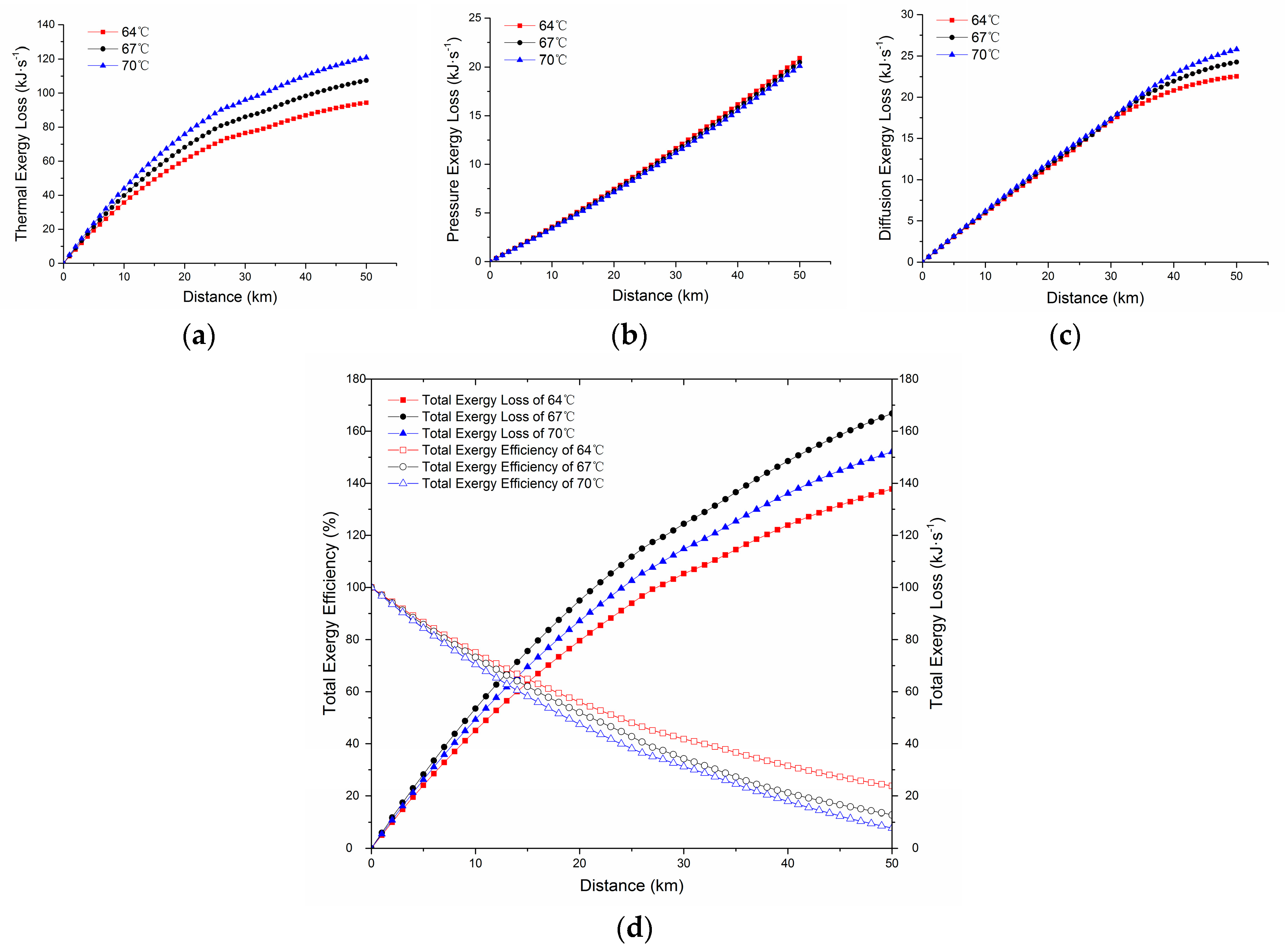
The axial distribution the curves of various exergy losses under different out-station temperatures are drawn in Figure 4.
From Figure 4, through analyzing various exergy losses under different out-station temperatures, we can draw the following conclusions. The higher the out-station temperature, the greater the thermal exergy loss, which can be explained as being due to the fact that the higher the out-station temperature, the larger the temperature difference between the oil and the surroundings, resulting in the greater thermal loss of crude oil. The higher the out-station pressure, the lower the pressure exergy loss, because high pressure reduces the viscosity of crude oil. The lower the out-station temperature, the larger the diffusion exergy loss. When the oil along the pipeline has a low temperature, the wax molecules originally in the dissolved state begin to precipitate and deposit. The diffusion and precipitation of the wax molecules all consume a part of the chemical potential as the driving force, so the chemical potential of the oil flow reduces, and the diffusion exergy loss becomes larger. The thermal exergy loss and diffusion exergy loss change a lot, and the proportion of pressure exergy loss is relatively small, so both the change of total exergy loss and total exergy efficiency become larger.
4.4.2. The Axial Distribution of Various Exergy Losses under Different Out-Station Pressures
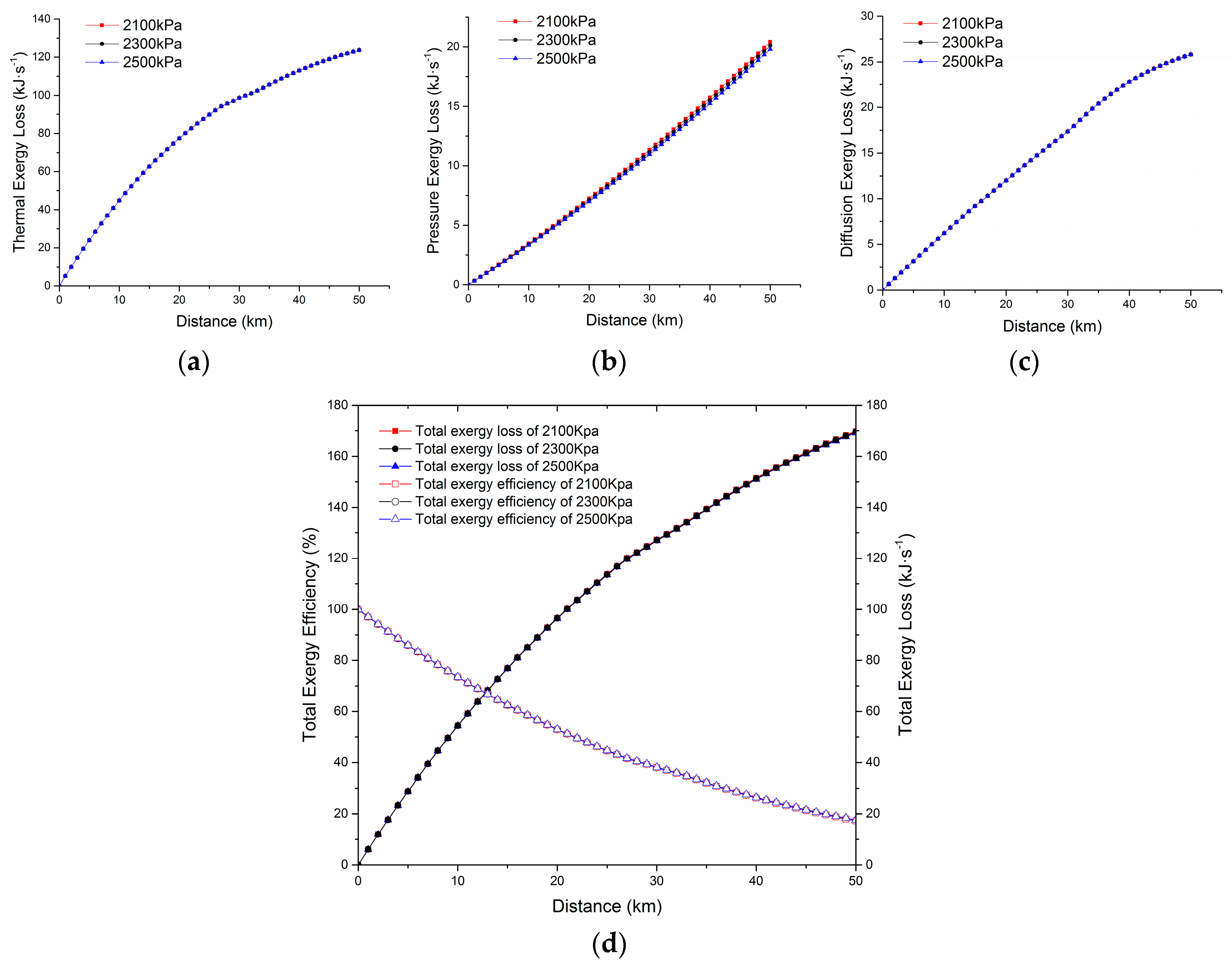
The axial distribution curves of various exergy losses under different out-station pressures are drawn in Figure 5.
From Figure 5, through analyzing various exergy losses under different out-station pressures, it can be shown that different out-station pressures have little effect on thermal exergy loss, diffusion exergy loss and total exergy loss, but they do impact the pressure exergy loss, though this is very small. The reason for this is that the out-station pressure has little effect on the temperature drop along the pipeline, but it has some effects on the pressure drop. In addition, the lower the out-station pressure, the larger the pressure exergy loss. The possible reasons for this can be summarized as follows. When the out-station pressure is low, the temperature drop along the pipeline is large, and the viscosity of the crude oil increases, leading to an increase of pressure exergy loss. As the diffusion exergy loss is mainly affected by the temperature field, the corresponding change of diffusion exergy loss is very small. Compared with the thermal exergy loss and the diffusion exergy loss, the pressure exergy loss accounts for a smaller proportion, resulting in the corresponding total exergy loss and total exergy efficiency changing little.
4.4.3. The Axial Distribution of Exergy Loss under Different Flow Rates
The axial distribution curves of various exergy losses under different flow rates are drawn in Figure 6.
From Figure 6, through analyzing various exergy losses under different flow rates, we can draw the following conclusions. The larger the pipeline flow rate, the smaller the thermal exergy loss, because the increase of velocity will decrease the external heat loss of the pipeline. The larger the pipeline flow rate, the bigger the pressure exergy loss, because the decrease of pipeline flow rate will lead to an increase of friction loss. The larger the pipeline flow rate, the smaller the diffusion exergy loss, which is due to the fact that the temperature drop along the pipeline decreases with the increase in the pipeline flow rate, the high oil temperature leads to a small amount of corresponding wax precipitation, and the consumption of chemical potential reduces accordingly. Various types of exergy losses and total exergy efficiency change little under different flow rates, which shows that the flow rate has little effect on various types of exergy loss along the pipeline transportation.
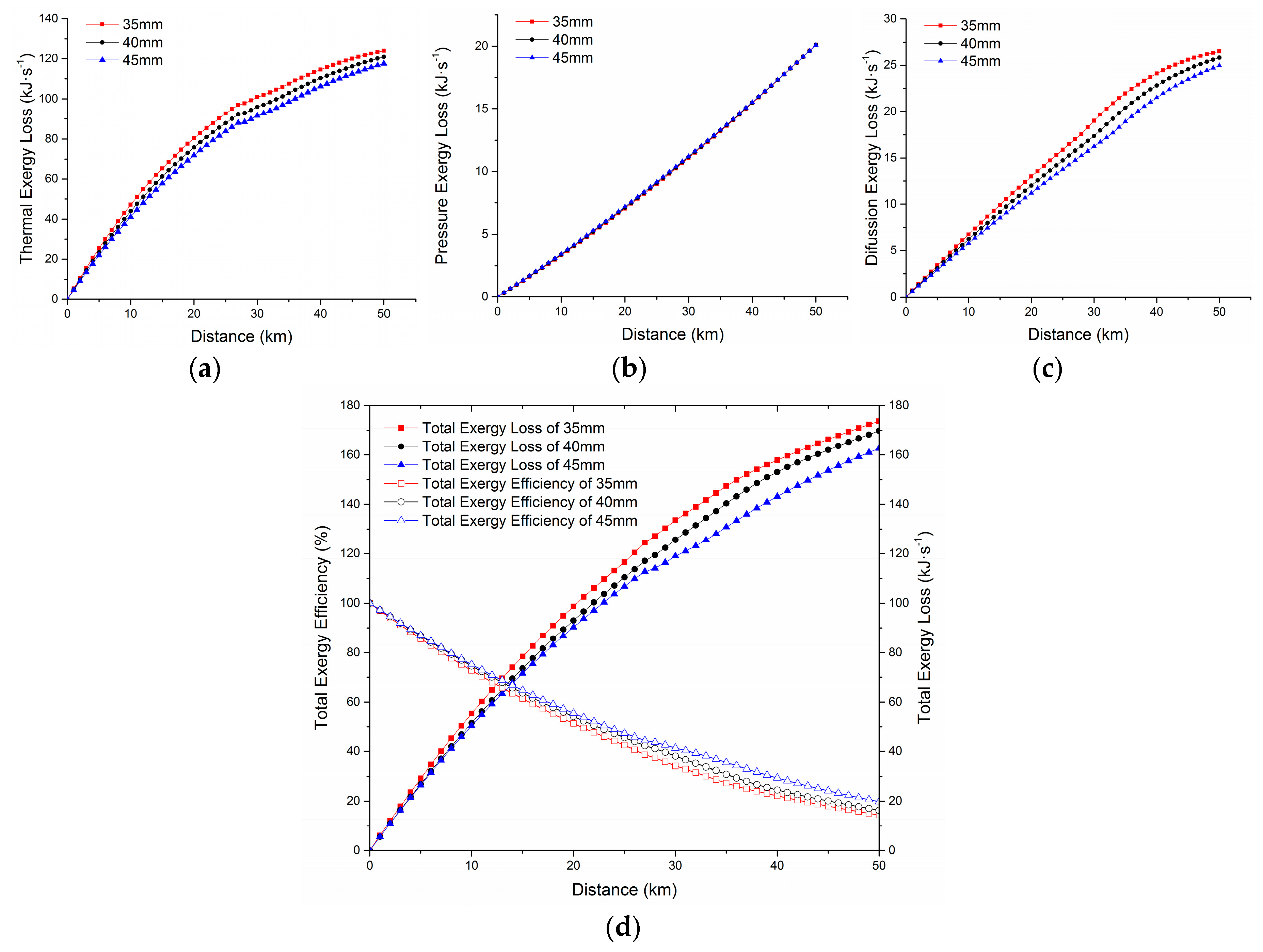
The axial distribution curves of various exergy losses under different insulation thicknesses are drawn in Figure 7.
According to the analysis of the influence of different insulating layer thicknesses on various exergy losses along the pipeline, it can be seen that the thickness of the insulation layer has little influence on pressure exergy loss, but has a great effect on thermal exergy loss, diffusion exergy loss, total exergy loss and total exergy efficiency. It can be seen from the above figures, that the thicker the insulation layer, the smaller the thermal exergy loss, because with the increase of the insulation layer thickness, the heat loss of the pipeline decreases. The insulation layer thickness has little effect on the pressure exergy loss, because the pressure exergy is greatly affected by the transportation pressure, and the influence of temperature is relatively small. The thicker the insulation layer, the smaller the diffusion exergy loss, because the drop in temperature decreases with the increase of insulation layer thickness, the oil flow wax precipitation is smaller, and the chemical potential caused by the consumption of wax molecular diffusion and deposition decreases accordingly.
4.5. Analysis of the Total Exergy Efficiency of the Orthogonal Test
The axial distribution of all kinds of exergy losses under different conditions was analyzed in the above chapters, and the main reasons for these phenomena were pointed out, but the degree of influence of various conditions on the exergy loss is not clear, and it is necessary to analyze the degree of influence of each working condition by the orthogonal experiment method [25]. In this test, the 66 × 103 kg·h−1 design flow rate is adopted. Assuming no interaction between all kinds of conditions, three factors of the orthogonal table are selected. For the three factors and two levels of orthogonal experiment, there exists at least four experimental groups, which is expressed as L4 (23). The specific experimental scheme and results are shown in Table 3.
We applyied the range method to analyze the results, which are shown in Table 4.
It can be shown from the range analysis that, under the 66 × 103 kg·h−1 design flow rate, the order of the influence degree on total exergy efficiency under different working conditions are insulating layer thickness, out-station temperature and out-station pressure. From the aspect of reducing the total exergy loss of waxy crude oil pipeline transportation, the key for energy conservation work should be carried out according to the above orders. The combined scheme with the highest total exergy efficiency is: an out-station temperature of 65 °C, out-station pressure of 2500 kPa, and an insulation layer thickness of 45 mm. Through calculating the program, obtained a total exergy efficiency of 20.68%, higher than the results of four tests which have been carried out, which shows that the scheme can achieve the optimum goal [26].
5. Conclusions
- The physical exergy values for the oil flow in the pipeline transportation process were the state parameters. When the environmental state was given, the thermal exergy was only a function of temperature, but it was associated with the physical properties Cp of the crude oil. The pressure exergy of the oil flow was a function of both temperature and pressure, and it had nothing to do with the properties of crude oil. The pressure exergy decreased with the increase of the temperature, and increased with the increasing of pressure.
- The chemical reaction exergy is generally calculated by approximation algorithms in the process of waxy crude oil transportation. However, this proportion was so small that it can be ignored in actual engineering calculations. The chemical diffusion exergy had an association with the chemical potential of the crude oil components. When the temperature of the oil dropped to the wax precipitation point, the wax molecules in the crude oil precipitated extensively, and with the decrease of temperature, the amount of wax precipitation increased, and the molecular concentration gradient changed intensively, resulting in a great change of chemical diffusion exergy.
- Taking a waxy crude oil transportation pipeline from an eastern Chinese oilfield as an example, the distribution of various types of exergy loss was studied. The results showed that along the waxy crude oil pipeline, all kinds of axial exergy losses were increasing, the thermal exergy loss was far greater than the pressure exergy loss and diffusion exergy loss, and the difference between the diffusion exergy loss and the pressure exergy was small. It was illustrated that the waxy crude oil transmission was greatly affected by the temperature field, the effect of the wax concentration field on the transportation process was in the second place, and the effect of the pressure field was the smallest. Compared with the external exergy loss, the internal exergy loss accounted for a smaller proportion. The internal exergy loss was often caused by an irreversible process, and we can only attempt to reduce, but not eliminate it.
- The orthogonal analysis method was used to analyze the degree of influence of various factors on the total exergy efficiency. The results showed that under different working conditions, the orders of the influence degree on out-station total exergy efficiency were: insulation layer thickness, out-station temperature and out-station pressure. It was confirmed that the highest combination scheme for total exergy efficiency under the 66 × 103 kg·h−1 design flow rate was an out-station temperature of 65 °C, an out-station pressure of 2500 kPa, and an insulation layer thickness of 45 mm.
Acknowledgments
This work was financially supported by the National Natural Science Foundation of China (51534004), the Northeast Petroleum University Innovation Foundation for Postgraduates (YJSCX2015-009NEPU).
Author Contributions
Yang Liu developed the study conception; Qinglin Cheng developed the design and produced the mathematical models; Yifan Gan calculated the cases by the produced mathematical models; Wenkun Su analyzed the results and gave the conclusions; Wei Sun and Ying Xu carried out the literature survey.
Conflicts of Interest
The authors declare no conflict of interest.
Abbreviations
The following abbreviations are used in this manuscript:
| E | exergy (kJ) |
| W | work (kJ) |
| R | constant of ideal gas (-) |
| T | temperature (K) |
| V | molar volume (m3/mol) |
| K | constant of the liquid-solid equilibrium (-) |
| H | enthalpy (kJ) |
| C | relative molecular mass (-) |
| M | molar mass (g/mol) |
| G | mass (kg) |
| Q | flow rate (m3/s) |
| S | entropy (kJ/K) |
| e | specific exergy (kJ/kg) |
| c | specific heat capacity (kJ/kg·K) |
| d | relative density (-) |
| p | pressure (kPa) |
| ρ | density (kg/m3) |
| n | mole number (mol) |
| x | molar fraction (-) |
| r | activity coefficient (-) |
| f | fugacity (-) |
| Greek Symbols | |
| ξ | temperature coefficient (-) |
| μ | chemical potential (kJ/mol) |
| δ | solubility parameter (-) |
| η | exergy efficiency (-) |
| ψ | exergy loss coefficient (-) |
| Subscripts | |
| xph | physical |
| xt | thermal |
| xp | pressure |
| 0 | initial state |
| xch | chemical |
| C | chemical reaction |
| D | chemical diffusion |
| i | component |
| x,gain | gained |
| x,pay | paid |
| L | loss |
| Superscripts | |
| 0 | initial state |
| L | liquid |
| S | solid |
| SL | liquid-solid |
| f | fugacity |
References
- Tang, X.; McLellan, B.C.; Zhang, B.S.; Snowden, S.; Hook, M. Trade-off analysis between embodied energy exports and employment creation in China. J. Clean. Prod. 2016, 134, 310–319. [Google Scholar] [CrossRef]
- Yang, X.H.; Zhang, G.Z. Design and Management of Oil Pipeline; China University of Petroleum Press: Dongying, China, 1996; pp. 121–166. ISBN 9787563608669. [Google Scholar]
- Sun, X.L. Analysis on Entropy Production Rate in Pipeline Process of Waxy Crude Oil. Master’s Thesis, North East Petroleum University, Daqing, China, 2013. [Google Scholar]
- Han, G.Z.; Guo, P.S.; Li, S.X.; Hua, B. Thermodynamic exergy and dynamic characteristics of its generalized expressions. J. Eng. Therm. Eng. Power 2007, 22, 409–413. [Google Scholar] [CrossRef]
- Enrico, S.; Göran, W. A brief commented history of exergy from the beginnings to 2004. Int. J. Thermodyn. 2007, 10, 1–26. [Google Scholar] [CrossRef]
- Kenhuanhui of Energy Transformation. Technology for Effective Use of Energy; Chemical Industry Press: Beijing, China, 1984; ISBN 9787109178373. [Google Scholar]
- Zhu, M.S. The Analysis of Energy System by Exergy; Tsinghua University Press: Beijing, China, 1988; ISBN 7-302-00015-8. [Google Scholar]
- Chaczykowski, M.; Osiadacz, A.J.; Uilhoorn, F.E. Exergy-based analysis of gas transmission system with application to Yamal-Europe pipeline. Appl. Energy 2011, 88, 2219–2230. [Google Scholar] [CrossRef]
- Ameri, M.; Askari, M. Enhancing the efficiency of crude oil transportation pipeline: A novel approach. Int. J. Exergy 2013, 13, 523–542. [Google Scholar] [CrossRef]
- Cheng, Q.L.; Ding, N.; Yi, X.; Zhao, Y.; Sun, W. Study of exergy and conversion law of irreversible process in crude oil pipeline transportation. J. Therm. Sci. Technol. 2015, 14, 125–129. [Google Scholar] [CrossRef]
- Gooya, R.; Gooya, M.; Dabir, B. Effect of flow and physical parameters on the wax deposition of middle east crude oil under subsea condition: Heat transfer viewpoint. Heat Mass Transf. 2013, 49, 1205–1216. [Google Scholar] [CrossRef]
- Fu, Q.S. Thermodynamic Analysis Method of Energy System; Xi’an Jiaotong University Press: Xi’an, China, 2005; ISBN 9787560519449. [Google Scholar]
- Chen, W.H.; Zhao, Z.C. Thermodynamic modeling of wax precipitation in crude oils. Chin. J. Chem. Eng. 2006, 14, 685–689. [Google Scholar] [CrossRef]
- Xiang, X.Y.; Cheng, Q.L. Entropy, exergy and energy analysis, energy transfer. J. Therm. Sci. Technol. 2004, 3, 275–278. [Google Scholar] [CrossRef]
- Kaushik, S.C.; Singh, O.K. Estimation of chemical exergy of solid, liquid and gaseous fuels used in thermal power plants. J. Therm. Anal. Calorim. 2014, 115, 903–908. [Google Scholar] [CrossRef]
- Gupta, A.; Anand, Y.; Anand, S.; Tyagi, S.K. Thermodynamic optimization and chemical exergy quantification for absorption-based refrigeration system. J. Therm. Anal Calorim. 2015, 122, 893–905. [Google Scholar] [CrossRef]
- Su, W.K. The Comprehensive Composition of Exergy Flow and Exergy Loss Analysis in Waxy Crude Oil Transportation Process. Master’s Thesis, North East Petroleum University, Daqing, China, 2016. [Google Scholar]
- Govin, O.V.; Diky, V.V.; Kabo, G.J.; Blokhin, A.V. Evaluation of the chemical exergy of fuels and petroleum fractions. J. Therm. Anal. Calorim. 2000, 62, 123–133. [Google Scholar] [CrossRef]
- Chen, W.H. The Thermodynamic Research of Wax Precipitation in Crude Oils. Master’s Thesis, Dalian University Technology, Dalian, China, 2006. [Google Scholar]
- Cai, J.M.; Zhang, G.Z.; Xing, X.K.; Luo, J.W. Research developments of wax deposition in waxy crude oil pipelines. Oil Gas Storage Transp. 2002, 21, 12–16. [Google Scholar] [CrossRef]
- Han, G.Z.; Hua, B.; Chen, Q.L.; Yin, Q.H. The general expression of exergy in thermodynamics. Sci. China (Ser. A) 2001, 31, 934–938. [Google Scholar] [CrossRef]
- Weingarten, J.S.; Euchner, J.A. Methods for predicting wax precipitation and deposition. SPE Prod. Eng. 1988, 3, 121–126. [Google Scholar] [CrossRef]
- Pedersen, K.S.; Skovborg, P. Wax precipitation from North-Sea crude oils. 4. Thermodynamic modeling. Energy Fuels 1991, 5, 924–935. [Google Scholar] [CrossRef]
- Li, Y.P.; Jia, M.; Chang, Y.C.; Kokjohn, S.L.; Reitz, R.D. Thermodynamic energy and exergy analysis of three different engine combustion regimes. Appl. Energy 2016, 180, 849–858. [Google Scholar] [CrossRef]
- Su, L.S.; Zhang, J.B.; Wang, C.J.; Zhang, Y.; Li, Z.; Song, Y.; Jin, T.; Ma, Z. Identifying main factors of capacity fading in lithium ion cells using orthogonal design of experiments. Appl. Energy 2015, 163, 201–210. [Google Scholar] [CrossRef]
- Zhao, B.; Shi, C.J.; Yang, X.F.; Gao, D.K.; Xu, L.Z.; Zhang, Y.Y. Temperature field analysis of liquid stratification for LNG tank based on orthogonal ridgelet finite element method. J. Therm. Anal. Calorim. 2016, 125, 557–562. [Google Scholar] [CrossRef]
Figure 1.
The exergy analysis model in the process of pipeline transportation.

Figure 2.
(a) The ratios of various exergy losses to total exergy loss; (b) The ratios of internal exergy loss and external exergy loss to total exergy loss.
Figure 2.
(a) The ratios of various exergy losses to total exergy loss; (b) The ratios of internal exergy loss and external exergy loss to total exergy loss.
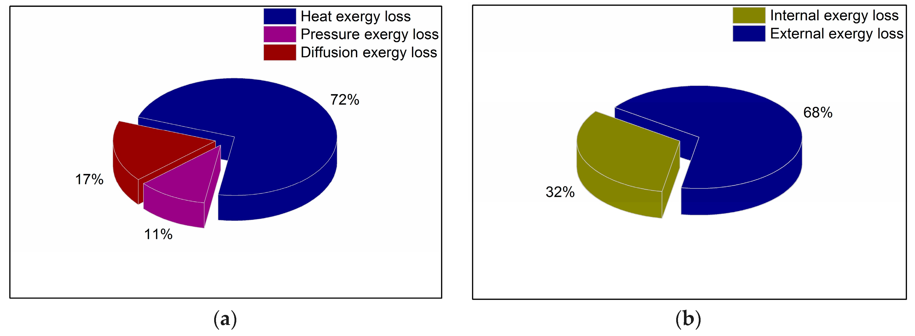
Figure 3.
The axial distribution curve of exergy losses.

Figure 4.
(a) The axial distribution of thermal exergy loss under different out-station temperatures; (b) The axial distribution of pressure exergy loss under different out-station temperatures; (c) The axial distribution of diffusion exergy loss under different out-station temperatures; (d) The axial distribution of total exergy loss/efficiency under different out-station temperatures.

Figure 5.
(a) The axial distribution of thermal exergy loss under different out-station pressures; (b) The axial distribution of pressure exergy loss under different out-station pressures; (c) The axial distribution of diffusion exergy loss under different out-station pressures; (d) The axial distribution of total exergy loss/efficiency under different out-station pressures.

Figure 6.
(a) The axial distribution of thermal exergy loss under different flow rates; (b) The axial distribution of pressure exergy loss under different flow rates; (c) The axial distribution of diffusion exergy loss under different flow rates; (d) The axial distribution of total exergy loss/efficiency under different flow rates.
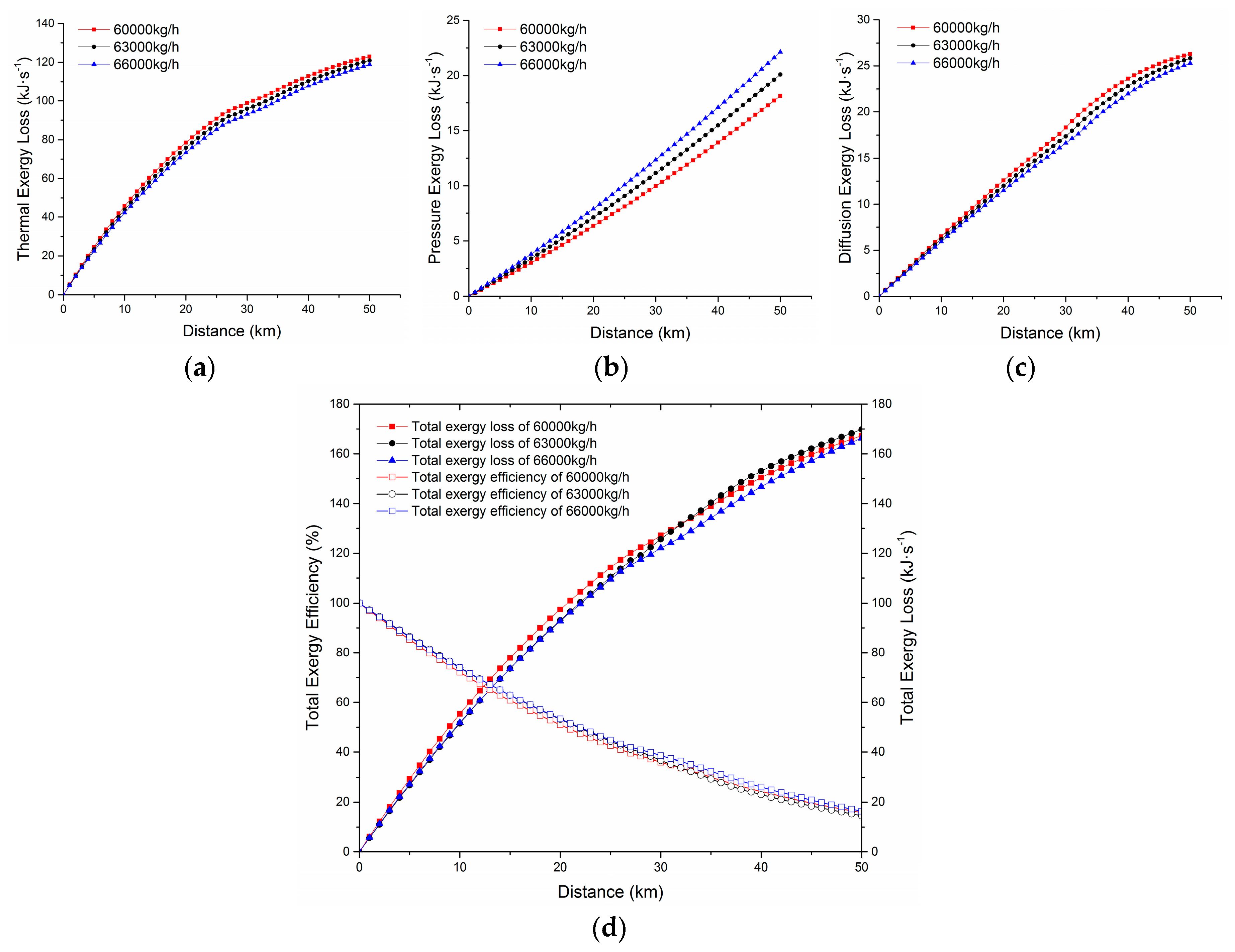
Figure 7.
(a) The axial distribution of thermal exergy loss under different insulation thicknesses; (b) The axial distribution of pressure exergy loss under different insulation thicknesses; (c) The axial distribution of diffusion exergy loss under different insulation thicknesses; (d) The axial distribution of total exergy loss/efficiency under different insulation thicknesses.

Table 1.
Pipeline operating parameters and physical parameters of the crude oil.
| Items | Numerical Value |
|---|---|
| Operating time, day | 350 |
| Thickness of insulating layer, mm | 40 |
| Thermal conductivity of insulating layer, W·m−1·°C−1 | 0.025 |
| Thermal conductivity of soil, W·m−1·°C−1 | 1.4 |
| Pipeline thermal conductivity, W·m−1·°C−1 | 45.24 |
| Pipe length, km | 50 |
| Pipeline diameter, mm | 207.9 |
| Top of the pipe buried depth, mm | 1600 |
| Environment temperature, °C | −4 |
| Absolute roughness, mm | 0.15 |
| Thickness of pipeline, mm | 5.6 |
| Out-station pressure, kPa | 2300 |
| Out-station temperature, °C | 70 |
| Flow rate, kg/h | 63,000 |
| Density of waxy crude oil at 20 °C, kg·m−3 | 844.1 |
| Wax content of waxy crude oil, % | 20.2 |
| Wax precipitation point, °C | 48 |
| Abnormal point, °C | 36.2 |
Table 2.
Comparison table of parameters under different working conditions.
| Conditions | Out-Station Temperature °C | Out-Station Pressure kPa | Flow Rate 103 kg·h−1 | Thickness of Insulating Layer mm |
|---|---|---|---|---|
| Condition1 | 70 | 2500 | 66 | 45 |
| Condition 2 | 65 | 2300 | 63 | 40 |
| Condition 3 | 60 | 2100 | 60 | 35 |
Table 3.
The results of the orthogonal experiment.
| Working Condition | Out-Station Temperature (°C) | Out-Station Pressure (kPa) | Thickness of Insulation Layer (mm) | Total Energy Efficiency (%) | ||
|---|---|---|---|---|---|---|
| Level | ||||||
| Test Number | ||||||
| 1 | 70 | 2500 | 45 | 18.94 | ||
| 2 | 70 | 2300 | 40 | 17.17 | ||
| 3 | 65 | 2500 | 40 | 18.15 | ||
| 4 | 65 | 2300 | 45 | 18.73 | ||
Table 4.
Range analysis of total exergy efficiency.
| Condition Category | Out-Station Temperature | Out-Station Pressure | Thickness of Insulation Layer |
|---|---|---|---|
| T1j | 36.11 | 37.09 | 37.67 |
| T2j | 36.88 | 35.90 | 35.32 |
| Rj | 0.77 | 1.19 | 2.35 |
© 2017 by the authors. Licensee MDPI, Basel, Switzerland. This article is an open access article distributed under the terms and conditions of the Creative Commons Attribution (CC BY) license (http://creativecommons.org/licenses/by/4.0/).
Share and Cite
MDPI and ACS Style
Cheng, Q.; Gan, Y.; Su, W.; Liu, Y.; Sun, W.; Xu, Y. Research on Exergy Flow Composition and Exergy Loss Mechanisms for Waxy Crude Oil Pipeline Transport Processes. Energies 2017, 10, 1956. https://doi.org/10.3390/en10121956
AMA Style
Cheng Q, Gan Y, Su W, Liu Y, Sun W, Xu Y. Research on Exergy Flow Composition and Exergy Loss Mechanisms for Waxy Crude Oil Pipeline Transport Processes. Energies. 2017; 10(12):1956. https://doi.org/10.3390/en10121956
Chicago/Turabian StyleCheng, Qinglin, Yifan Gan, Wenkun Su, Yang Liu, Wei Sun, and Ying Xu. 2017. "Research on Exergy Flow Composition and Exergy Loss Mechanisms for Waxy Crude Oil Pipeline Transport Processes" Energies 10, no. 12: 1956. https://doi.org/10.3390/en10121956
Note that from the first issue of 2016, this journal uses article numbers instead of page numbers. See further details here.